Evaluating the potential for efficient, UAS-based reach-scale mapping of river channel bathymetry from multispectral images

1 Introduction

Remote sensing plays an increasingly prominent role in the river community as researchers and practitioners seek to more thoroughly understand and effectively manage channels, floodplains, and riparian corridors across a range of spatial scales from small study sites to entire watersheds (Marcus and Fonstad, 2010; O’Sullivan et al., 2021). The advent of this approach has fostered development of the riverscape concept (Carbonneau et al., 2012) and generated optimism regarding the contribution remote sensing could make toward our understanding of rivers as fluvial systems face challenges associated with anthropogenic effects and other aspects of environmental change (Tomsett and Leyland, 2019; Piégay et al., 2020). Fully realizing this potential will require careful, systematic assessment of not only the capabilities of image-based methods for characterizing rivers but also their inherent limitations. This study focuses on one such application, mapping spatial patterns of water depth in rivers using multispectral image data acquired from uncrewed aircraft systems (UAS). Reasons for focusing on depth include the importance of this attribute in (1) determining the suitability of in-stream habitat for various species throughout their life histories and (2) dictating the erosion, transport, and deposition of sediment, which in turn drive a channel’s morphologic evolution.

Building upon early work in coastal environments (e.g., Lyzenga, 1978), estimating water depth from passive optical image data has become one of the more mature applications of remote sensing to rivers. Although the marine research community has explored more sophisticated radiative transfer modeling-based approaches that could obviate the need for in situ depth measurements (e.g., Mobley et al., 2005), remote sensing of river bathymetry remains primarily an empirical endeavor. For example, Winterbottom and Gilvear (1997) demonstrated that a continuous depth map could be produced by regressing pixel values against co-located, field-based depth measurements and then applying the resulting equation throughout the image. Although more advanced statistical methods, such as the Gaussian mixture model-based clustering of Kwon et al. (2023) or the deep neural network of Niroumand-Jadidi et al. (2022), are now employed, the basic premise is unchanged: image-derived quantities are related to depth via a training process that requires in situ observations for calibration.

One widely used implementation of this general workflow is the Optimal Band Ratio Analysis (OBRA) framework introduced by Legleiter et al. (2009) and subsequently expanded upon by Legleiter and Harrison (2019). Though also empirical in nature, OBRA has a solid physical foundation based on the interaction of light and water (Mobley, 1994). OBRA establishes a relationship between depth and reflectance by exploiting variations in the rate at which solar radiation is attenuated as it propagates through the water column, first toward the bed and then back up toward the water surface after reflecting off the bottom. The spectral radiance measured by a remote detector thus depends not only on depth but also the reflectance of the streambed. Additional components of the radiance signal include light scattered into the field of view by the atmosphere and/or adjacent terrestrial features, reflection from the water surface (i.e., sun glint), and volume reflectance from within the water column, as influenced by any suspended or dissolved constituents therein. However, under appropriate environmental conditions—primarily clear, relatively shallow water—and for certain combinations of wavelengths, Legleiter et al. (2009) showed that a log-transformed band ratio can effectively isolate the effect of depth. The OBRA algorithm described in greater detail below thus takes as input paired observations of depth and reflectance and identifies the numerator and denominator wavelengths that yield the strongest relationship between an image-derived quantity and water depth.

The OBRA framework has been successfully applied across a range of fluvial environments, including supraglacial streams (Legleiter et al., 2014), sand-bed channels (Dilbone et al., 2018), and large but clear-flowing rivers approaching 10 m in depth (Legleiter and Fosness, 2019). Data sets used in these studies range from publicly available aerial photos (Legleiter, 2013) to hyperspectral images with over 40 narrow bands (Legleiter et al., 2018). In addition to conventional, fixed-wing aircraft, OBRA-based bathymetric maps have been generated from images acquired from spaceborne platforms (Legleiter and Overstreet, 2012) and small multi-rotor UAS (Legleiter and Harrison, 2019). Although some refinements to the OBRA algorithm—for example, incorporating multiple band ratio predictors that vary as a function of depth (Niroumand-Jadidi et al., 2020) — have been proposed and might yield some marginal improvement in performance, the core framework has proven to be robust and flexible over more than a decade of application. Another important advantage of OBRA is its availability within a free, standalone software package: the Optical River Bathymetry Toolkit (ORByT) (Legleiter, 2021). This program enables end users who have neither experience in remote sensing nor access to specialized software to take an image in a standard file format such as a GeoTIFF, along with field-based depth measurements, and, within a few minutes, produce a bathymetric map. Another ORByT module allows users to create a fused topo-bathymetric digital elevation model (DEM) by combining the depth map with lidar data that provide information on the elevation of the water surface and adjacent terrestrial areas.

In this study, we used the well-established OBRA depth retrieval workflow to evaluate the potential to efficiently map river channel bathymetry via UAS. However, an important caveat to bear in mind from the outset is that this spectrally based approach is only possible under a very limited range of river conditions. These conditions can be specified most rigorously in terms of the inherent optical properties of the water column (Legleiter et al., 2018) but essentially amount to clear water with low concentrations of suspended sediment, chlorophyll, colored dissolved organic matter, and any other optically significant constituents. In addition, the range of depths that can be mapped via passive optical remote sensing is limited due to the finite radiometric sensitivity of digital imaging systems (Philpot, 1989; Legleiter and Fosness, 2019) and is thus restricted to relatively shallow, small-to medium-sized rivers with depths on the order of a few meters. The reach of the Sacramento River that we selected for this study satisfies these requirements and thus provides an appropriate venue to assess the feasibility of using UAS to support operational mapping of depth. In many other larger, deeper, and/or more turbid rivers, however, incontrovertible physical constraints would preclude this approach entirely.

Although the utility of UAS for measuring surface flow velocities in rivers has been highlighted in a number of recent studies (e.g., Dal Sasso et al., 2021; Strelnikova et al., 2023), their use for depth retrieval has received relatively little research attention (Harrison et al., 2020). These platforms have important advantages in terms of agility and flexibility compared to conventional aircraft, which typically require coordination with flight contractors and thus long lead times, or satellites, which provide only relatively coarse pixel sizes, have revisit times on the order of days to weeks, and are subject to cloud cover and atmospheric effects. In addition, their relatively low cost and ease of deployment could make UAS a viable option for operational river monitoring. Conversely, recognized limitations of UAS include their limited payload capacity, which restricts the range of sensors that can be deployed in this manner; the complex and shifting regulatory framework governing UAS operations, which often constrains their use to low altitudes within visual line of sight of the operator, reducing the area that can be covered in a single flight; and the short flight times supported by current battery technology, which also limits coverage.

The overarching objective of this investigation is to evaluate the potential to efficiently map the bathymetry of river reaches several kilometers in length via UAS-based remote sensing. Whether for research purposes or for routine monitoring, maximizing the rate at which information on water depths can be produced is desirable. We considered two ways of achieving this goal. First, if a depth retrieval model could be calibrated using data from one subset of the reach and then applied with confidence to a second, nearby sub-reach, the amount of field data required could be reduced significantly. Similarly, if the number of field observations could be decreased without compromising the accuracy of the image-derived bathymetry, further savings of time and effort could be realized. Motivated by this line of reasoning, we focus our attention herein on two specific aims: (1) Assess whether a relationship between depth and reflectance established for one sub-reach can yield reliable depth estimates when applied to a second, nearby area of interest; and (2) Infer the level of field effort required to support UAS-based bathymetric mapping by evaluating different strategies for obtaining in situ observations needed for calibrating image-derived quantities to depth.

2 Materials and methods

2.1 Study area

This investigation focused on a 4 km reach of the Sacramento River located near the town of Glenn in California’s Central Valley (Figure 1). The Sacramento is the largest river in the state and the drainage area at a U.S. Geological Survey (USGS) gaging station located 34 km downstream at Colusa (USGS station number 11389500) is approximately 31,000 km² (U.S. Geological Survey, 2023). The river is a crucial source of water for urban and agricultural uses and supports three populations of Pacific salmon listed under the Endangered Species Act (Moyle et al., 2017). Various management agencies are thus tasked with making critical decisions regarding water allocation within the Sacramento River basin. These decisions are based in part on a series of coupled physical-biological models developed for evaluating the impacts of water operations, fisheries management, and environmental variability on salmon population dynamics (Daniels and Danner, 2020; Dudley et al., 2022). Currently, a key limitation of these decision support tools is the lack of continuous, high-quality river bathymetry data that could serve as input to multidimensional hydrodynamic models (Harrison et al., 2022).

Figure 1

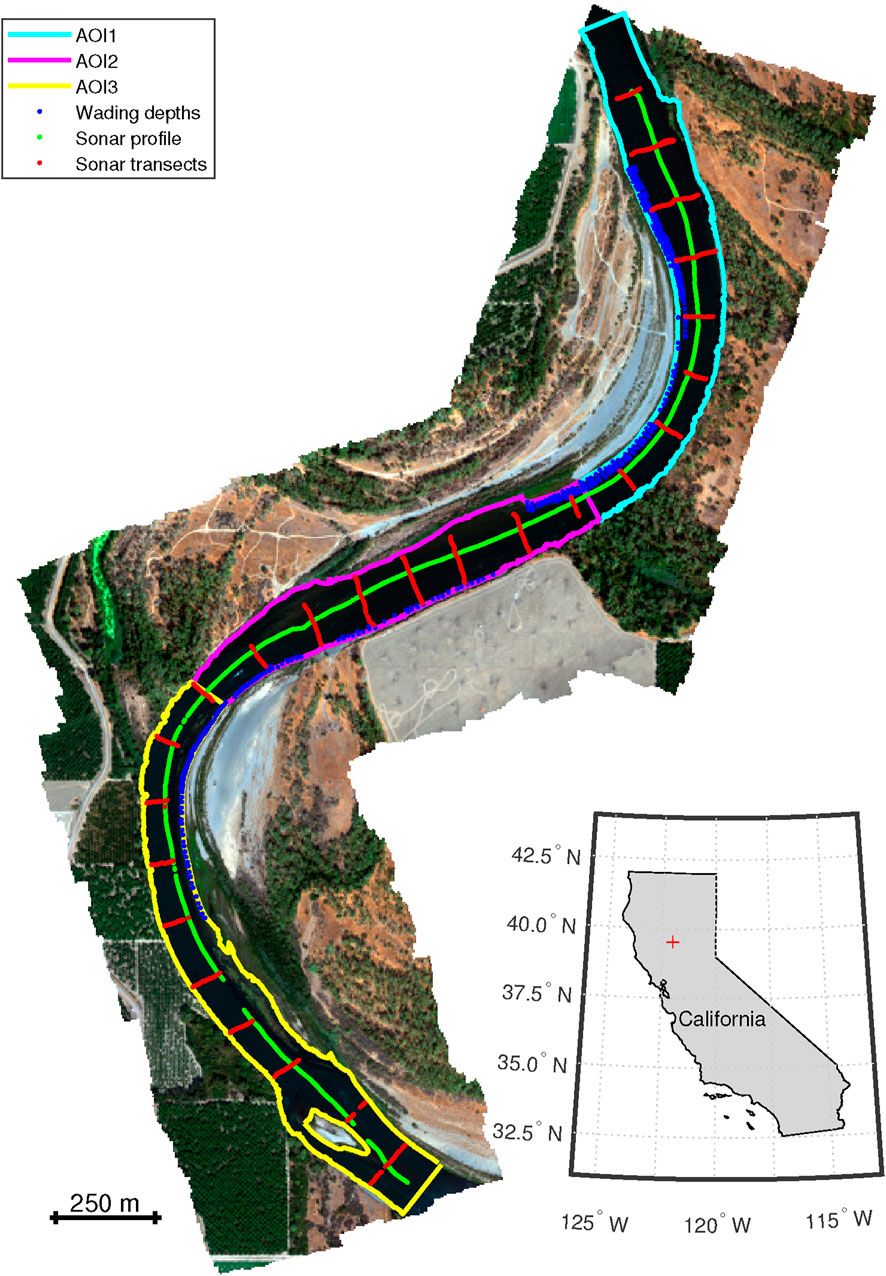
Figure 1. Overview of study area along the section of the Sacramento River indicated by the red + symbol on the inset map. The study area was divided into three separate sub-reaches or areas of interest (AOIs), each with a corresponding multispectral image. AOIs one, two, and three are represented by cyan, magenta, and yellow polygons, respectively. The three types of measurement of water depth collected in the field are represented by point symbols with wading points in blue, the longitudinal profile surveyed from a boat via sonar in green, and sonar cross sections in red. Flow is from north to south, from the top to the bottom of this map as well as all subsequent figures.

Our study area encompasses a full meander wavelength, with one bend to the east followed by a curve to the west as the river flows south (Figure 1; Figure 2). The sinuous channel has a mean width of 110 m and a water-surface slope of 0.0004. The bed material is predominantly gravel and samples collected in the first of our three sub-reaches had a median grain size (D₅₀) of 19 mm, with 90% of the measured particles finer than the D₉₀ of 54 mm (Singer, 2008). The lithology of the river bed is homogenous throughout the reach, but the presence of submerged aquatic vegetation and benthic algae created local variations in bottom reflectance (Figure 2). For water year 2021, which began on 1 October 2020 and ended on 30 September 2021, the mean annual streamflow was 146 m³/s (U.S. Geological Survey, 2023). Remotely sensed data and field measurements of water depth were acquired over a 3-day period from 14 to 16 September 2021, during which time the mean daily streamflow decreased from 167 to 158 m³/s, corresponding to a reduction in stage of 0.098 m at the Colusa streamgage (U.S. Geological Survey, 2023). The study area was partitioned into three distinct sub-reaches, with each serving as a separate area of interest (AOI) for image acquisition. As shown in Figure 1, AOI one was located the farthest upstream, included the entrance to the first bend, and extended past the apex of the bend. AOI two was a straight sub-reach between the two bends. AOI three was located the farthest downstream and included the long, sweeping second bend and a small island near the downstream end of the study area.

Figure 2

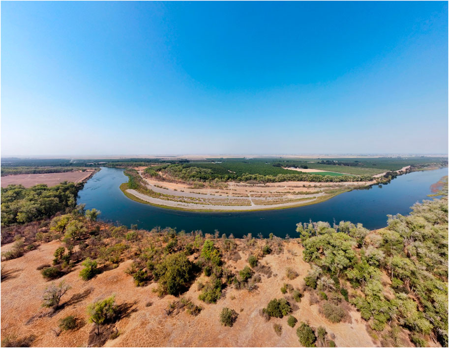
Figure 2. Photo of area of interest (AOI) one within the study area along the Sacramento River. This oblique photo was captured from an uncrewed aircraft system (UAS) from above the east bank, with a view toward the point bar on the west bank.

2.2 Field data

We obtained direct field measurements of water depth via wading surveys and from a jet boat. Collecting data while wading involved using real-time kinematic (RTK) Global Navigation Satellite System (GNSS) receivers to record water-surface elevations (WSEs) along the edge of the wetted channel and then bed elevations along transects oriented perpendicular to the primary channel flow direction. Water depths were calculated by subtracting each surveyed bed elevation from the nearest WSE observation. In the deeper portions of the channel that could not be waded safely, we measured depths along a longitudinal profile and 25 channel-spanning transects (i.e., cross sections) using a jet boat equipped with a single-beam echo sounder (Figure 1). Although the echo sounder allowed us to measure greater depths directly in the field, an important limitation of this instrument was its inability to measure depths shallower than about 0.4 m. For this reason, we hypothesized that a combination of shallow wading depths and echo sounder data from deeper areas would lead to the most accurate depth estimates. To evaluate this hypothesis, we evaluated different sampling configurations that made use of the two types of field measurements in varying proportions.

This field campaign yielded an extensive, detailed data set on water depth within the study area consisting of 3,260 point measurements. Depth distributions within each AOI and for each data type within AOI one are summarized graphically in Figure 3 and statistically in Table 1. The straight sub-reach in AOI two had the shallowest mean depth of 1.11 m, whereas the AOI one encompassing the first bend had a slightly greater mean depth of 1.24 m. The third AOI, which included the second bend and a pool over 4.5 m deep, had a much greater mean depth of 2.02 m and thus a much broader distribution of depths overall. These differences in depth among sub-reaches have important implications for bathymetric mapping that will be discussed later.

Figure 3

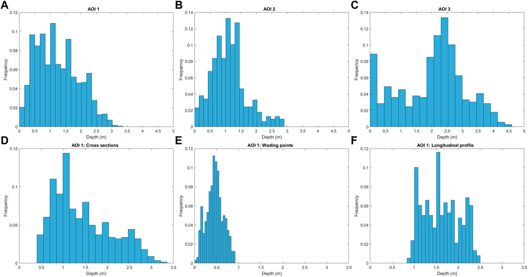
Figure 3. Histograms of water depth measurements made in the field, grouped first by area of interest (AOI) in panels (A–C) and then by type of data within AOI one in panels (D–F). Corresponding summary statistics are provided in Table 1. These data are available in Legleiter and Harrison (2023).

Table 1

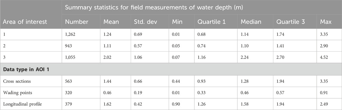
Table 1. Summary statistics for field measurements of water depth, stratified first by area of interest (AOI) and then by data type within AOI one. These data are available in Legleiter and Harrison (2023).

2.3 Remotely sensed data

2.3.1 UAS-based image acquisition

We acquired UAS-based multispectral image data using a Trinity F90+ vertical take-off and landing fixed-wing platform equipped with a MicaSense (AgEagle Aerial Systems Inc., Wichita, KS, USA) RedEdge-MX dual-camera imaging system. The Trinity F90+ was equipped with an onboard post-processed kinematic (PPK) system capable of providing centimeter-level horizontal and vertical positioning of geotagged images, with approximately 75 min of flight time when flying with a typical payload. The Trinity F90+ also allows for stable take-offs and landings, which is an important consideration in river corridors that often lack smooth terrain suitable for fixed-wing landings. The RedEdge-MX dual-camera system is a radiometrically calibrated spectral imager with ten bands between 400 and 900 nm. We anticipated that the RedEdge-MX dual-camera system would be useful for mapping water depth because the spectral bands of this sensor are comparable to those of the WorldView3 satellite, which we had used previously to produce accurate depth estimates for another reach of the Sacramento River farther upstream (Legleiter and Harrison, 2019).

We flew the Trinity F90+ at an altitude of 120 m, and collected multispectral imagery along a series of overlapping flight lines which covered the wetted channel and roughly 50 m of the floodplain on either side of the river. Flight duration was typically about 45 min, an amount of time sufficient to acquire image data covering roughly 1.5 km of the river channel. To account for differences in solar lighting between flights, we used the RedEdge-MX dual-camera system to record an image of a MicaSense calibrated reflectance panel immediately before and after each flight. Following the manufacturer’s recommendations, the panel was placed on the ground and the sensor held approximately 1 m above the target (MicaSense, 2023). The reflectance values of the calibration panel were 0.473 or 0.474 for each of the ten bands. All flights were conducted near solar noon and within visible line of sight of the UAS pilot. We geotagged the raw images using Quantum-Systems QBase 3D software (Quantum Systems, 2024). Agisoft Metashape was used to convert the raw image data to units of reflectance following MicaSense’s radiometric calibration guidelines (Agisoft, 2023) and then generate orthorectified image mosaics, which had pixel sizes of approximately 8 cm.

2.4 Spectrally based depth retrieval

To infer water depth from these multispectral images, we made use of the OBRA framework described in Section 1. Essentially, this approach is designed to isolate the effect of depth on the radiance signal and be relatively insensitive to the additional, confounding effects of reflectance from the water surface, the presence of any optically significant constituents other than pure water, and spatial variations in the reflectance of the streambed. OBRA involves defining an image-derived quantity X as

$X=\frac{\mathit{R}\left({\lambda }_1\right)}{\mathit{R}\left({\lambda }_2\right)},(1)$

where R (λ₁) and R (λ₂) are reflectance values in the numerator and denominator bands with center wavelengths denoted by λ₁ and λ₂, respectively. Given paired observations of spectral reflectance R(λ) and water depth d as input, the algorithm calculates values of X for all possible band combinations and then performs a regression of X against d for each version of X. The optimal band ratio is the (λ₁, λ₂) pair that yields the highest coefficient of determination R², and the corresponding regression equation serves as a depth retrieval model that can be applied throughout the image to produce a bathymetric map.

The initial formulation of OBRA considered only linear or quadratic relationships between X and d (Legleiter et al., 2009), but more recently Legleiter and Harrison (2019) generalized the approach by allowing for other, non-linear functional forms. One of these, an exponential model, avoids the negative depth estimates that can occur in shallow water if X is assumed to be linearly related to d and the overestimates of depth along the margins of the channel that can result from a quadratic X vs. d relation. This exponential model is given by

$d=b_0{e}^{b_{1}X},(2)$

where b₀ and b₁ are fitted coefficients. To estimate these parameters, this expression is linearized for regression purposes as

$\ln \left(d\right)=\ln \left(b_0\right)+b_{1}X.(3)$

In this form, b₁ is the slope of the best fit line on a plot of X vs. ln(d) and b₀ can be obtained by raising e to this line’s intercept. For this study, we performed exponential OBRA using source code from the ORByT software package (Legleiter, 2021).

2.4.1 Accuracy assessment

To assess the accuracy of depth estimates derived from multispectral images, we compared these estimates to measurements of water depth made directly in the field as described in Section 2.2. Prior to OBRA, the available field data were split into a calibration subset, which was used to develop the depth retrieval model, and a separate validation subset that was excluded from the training process and instead used to evaluate the performance of the resulting depth retrieval model. This validation involved performing observed vs. predicted (OP) regressions (Pineiro et al., 2008), where observed refers to the depths measured in the field and predicted refers to the image-derived estimates. A convenient summary of the degree to which these two quantities agree is the OP regression R², which ideally would be 1.0 if observed and predicted depths were perfectly matched. However, a high R² value does not necessarily indicate that the depth retrieval model is accurate, as a high R² can also result from a model that yields biased predictions (i.e., the slope and intercept of the OP regression could diverge from the ideal values of 1 and 0, respectively).

For this reason, we also used the validation subset of the field data to calculate depth retrieval errors as

$\epsilon =d_f-d_i,(4)$

where d_f is the field-measured depth and d_i is the image-derived depth. A positive value of ɛ thus indicates that the image-derived depth underestimated that measured in the field (i.e., was biased shallow), whereas negative values of ɛ occur where remotely sensed depths exceed the in situ observations and are thus biased deep. To provide a summary metric of any such systematic under- or overprediction of depth, we calculated the normalized bias by dividing the mean depth retrieval error by the reach-scale mean depth:

$\text{Normalized\hspace{0.17em}Bias}=\frac{1}{\overline{d_f}}\frac{{\sum }_{k=1}^n{\epsilon }_k}{n},(5)$

where $\overline{d_f}$ is the mean of the field-measured depths used for validation, n is the number of such observations, and ɛ_k denotes the error at location k. Similarly, we quantified the precision of the depth estimates in terms of the normalized root mean squared error (RMSE), calculated as

$\text{Normalized\hspace{0.17em}RMSE}=\frac{1}{\overline{d_f}}\sqrt{\frac{{\sum }_{k=1}^n{\epsilon }_k^2}{n}}(6)$

Normalizing in this manner allows both the accuracy and precision of image-derived depth estimates to be expressed as a proportion of the mean flow depth. To yield further insight regarding the frequency distribution and spatial structure of ɛ, we also examined histograms and maps of depth retrieval errors.

2.4.2 Assessing portability of depth-reflectance relations among sub-reaches

Initially, we applied the standard OBRA workflow described above independently for each of the three AOIs to yield a separate depth-reflectance relationship for each sub-reach of our study area along the Sacramento River. For this per-AOI analysis, we split all the field data available within each AOI evenly into calibration and validation subsets, with the former used to develop the depth retrieval model and the latter used to assess the accuracy of the resulting model. Although this single-site approach is straightforward and has been demonstrated through previous research, the first specific aim of this study was to assess whether an X vs. d relation established using data from one sub-reach could be applied to a second, distinct sub-reach and yield reliable bathymetric information for both areas. To investigate this possibility, we took the calibrated, OBRA-based depth retrieval model for each AOI and applied the model to the other two AOIs and used validation subsets of the field data from the latter AOIs to assess the accuracy of depth estimates derived using a version of Eq. 2 imported from a different sub-reach. Depth retrieval performance was quantified in terms of the three primary metrics defined above: OP R², normalized bias, and normalized RMSE.

2.5 Evaluating alternative sampling strategies for field data collection

The second specific aim stated in Section 1 was to assess whether the level of effort expended in the field to collect in situ observations of water depth for calibrating image-derived depth estimates could be reduced without compromising depth retrieval performance. For this phase of the investigation, we focused on AOI one and evaluated how alternative field data sets, made progressively more sparse relative to that we collected originally, would affect the accuracy and precision of image-derived depth estimates. The field data consisted of three different types of depth measurements: (1) observations from shallow areas along the channel margins acquired while wading with an RTK GNSS receiver; (2) cross sections surveyed with an echo sounder mounted on a boat; and (3) a longitudinal profile obtained from the same boat. The number of observations of each type is listed in Table 2. Before sub-sampling each type of data to produce different, sparser configurations, we first took the original, full field survey and removed half the points to serve as a validation subset. This approach ensured that a consistent set of points would be used to assess the accuracy of image-derived depth estimates across all the different sampling configurations we considered. Moreover, using a common validation subset drawn from all three types of observation allowed us to gain insight as to how depth retrieval performance might change in different parts of the channel as we manipulated the number and type of data used for calibration, including scenarios where certain types of data were excluded. For example, if we were to omit all wading observations from the calibration process, would depth retrieval performance in shallow areas be degraded? Setting aside a separate validation subset comprised of 50% of the available data of all three types allowed us to address questions of this kind.

Table 2

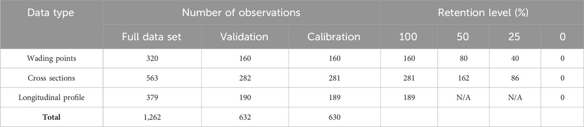
Table 2. Number of field observations from area of interest (AOI) one organized by data type, use for validation or calibration, and level of retention for evaluating different sampling configurations. Note that the number of observations for different levels of cross section retention are not exactly equal to the product of the total number of cross section calibration points (281) and the percent retained because all points along a given cross section were retained if the cross section was retained at all and the number of points varied among the eight cross sections. These data are available in Legleiter and Harrison (2023).

For the other half of the original field data set that were available for calibration, we considered a variety of different sampling strategies, all illustrated in Figure 4. These configurations were generated by progressively thinning each of the three types of field observation, independent of the other two data types. More specifically, we retained all, half, one-quarter, or none of the wading points. Similarly, we kept all, half, one-quarter, or none of the eight cross sections surveyed from the boat within AOI one. All points along a given cross section were included if that transect was retained and, conversely, all the points along a cross section were excluded if that transect was not retained as part of the calibration subset. The longitudinal profile was also treated in an all or nothing manner: we either retained all the points measured along the profile or none of them. The experimental design thus involved four levels of wading point retention, four levels of cross section retention, and two levels of longitudinal profile retention, yielding a total of 4 × 4 × 2 = 32 different sampling configurations.

Figure 4

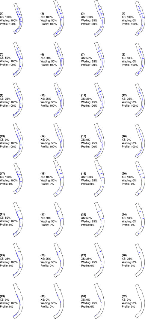
Figure 4. Sampling configurations used to evaluate the impact of the number and type of field-based depth measurements available for calibration on the performance of spectrally based depth retrieval.

The analysis was implemented by performing OBRA for all possible combinations of the four cross section scenarios, four wading scenarios, and two longitudinal profile scenarios. At each iteration of the innermost loop, a depth retrieval model was calibrated using the subset of field data retained for that particular sampling configuration and then applied to the validation subset, which, again, remained consistent throughout. Depth retrieval performance for each configuration was quantified in terms of the three primary metrics defined above: OP R², normalized bias, and normalized RMSE, with the results stored in 4 × 4 × 2 arrays with levels of cross section retention as rows, levels of wading data retention as columns, and levels of longitudinal profile retention as layers. These arrays were used to generate a series of summary plots to visualize how the accuracy and precision of image-derived depth estimates varied as a function of the number and type of field data used for calibration.

3 Results

3.1 Depth retrieval for individual sub-reaches

To assess the feasibility of spectrally based bathymetric mapping for this section of the Sacramento River, we first applied OBRA to each of the three images independently, using only field data from within that same AOI. Figure 5 shows an example of the output from this process for AOI one. The calibrated equation relating the image-derived quantity X, defined as the logarithm of the ratio of the reflectance in the green (560 nm) band to that in the red (650 nm) band, to depth is plotted in Figure 5A. The OBRA R² of 0.949 indicated a strong exponential relationship between depth and reflectance for depths up to 3 m for this AOI. Figure 5B provides further detail on spectral variations in the strength of the relationship between X and d by plotting the OBRA R² for all possible combinations of numerator and denominator bands. In this case, several other (λ₁, λ₂) pairs would have yielded R² values nearly as high as the optimum. For example, using the 650 nm band as the denominator with any numerator band with λ₁ < 650 nm also would have led to an OBRA R² > 0.9. The prevalence of bright yellow tones in Figure 5B indicates that the relationship between X and d was robust across a range of wavelengths and not restricted to a single, highly specific band combination. These results imply that under the low flow, clear water conditions observed at the time the image data for this study were acquired, this portion of the Sacramento River was conducive to spectrally based depth retrieval. The depth map produced by applying the calibrated OBRA relation is shown in Figure 5C and accurately depicts the morphology of this sub-reach: a deep, focused thalweg in the center of the channel at the entrance of the bend that shifts toward the outer bank as the channel curves, with shallower flow over the point bar on the inside of the bend.

Figure 5

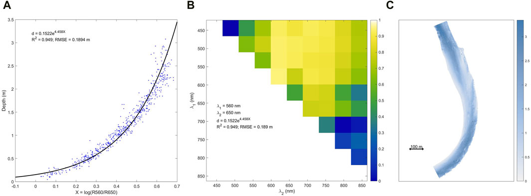
Figure 5. Example output from the Optimal Band Ratio Analysis (OBRA) depth retrieval algorithm for Area of Interest (AOI) one. (A) Calibrated exponential relationship between the image-derived quantity X and water depth d (B) Matrix plot illustrating spectral variations in the strength of the X vs. d relation for all combinations of numerator (λ₁) and denominator (λ₂) bands. (C) Depth map produced by applying the calibrated equation shown in (A) throughout the image.

We also performed similar, per-AOI OBRA for the other two sub-reaches of our study area and the results of these analyses are summarized in Table 3. Depth retrieval performance was consistently strong across all three AOIs, with OP R² values ranging from 0.915 for AOI three to 0.936 for AOI one. Normalized bias values were all less than about 1% of the mean depth within each AOI, indicating that image-derived depth estimates were minimally biased, with a slight tendency to underestimate the depths measured directly in the field. In addition, normalized RMSE values on the order of 15% implied that bathymetric maps of this portion of the Sacramento River produced via OBRA would also be highly precise, mainly because environmental conditions during image acquisition were favorable, with very clear water and depths generally less than about 3 m.

Table 3

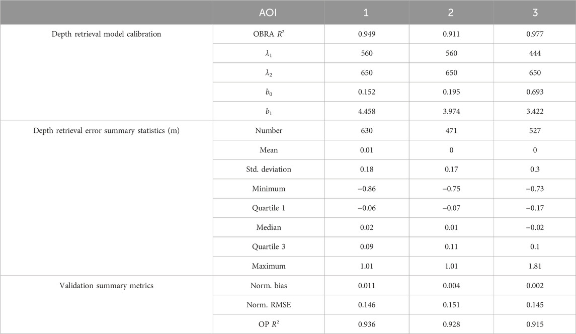
Table 3. Results of depth retrieval model calibration and validation for each area of interest (AOI) using only data from within that same AOI. These data are available in Legleiter and Harrison (2023).

Closer inspection of Table 3, however, suggested that of the three AOIs, the third sub-reach, located the farthest downstream, was the most problematic. Although the OBRA R² of 0.977 for AOI three was higher than the other two AOIs, indicating a very strong relationship between X and d, this high R² was at least partially a consequence of the broader range of depths present in this sub-reach, including a pool over 4.5 m deep (Figure 3; Table 1). As a result, a shorter-wavelength numerator band centered at 444 nm was selected as optimal. Blue light penetrates more efficiently through the water column than green or red radiation that is more strongly attenuated, which leads to saturation of the radiance signal in deeper water. However, strong attenuation of red wavelengths also made the band centered at 650 nm highly sensitive to variations in depth, which led to the red band being identified as the optimal denominator wavelength in all three AOIs. Beyond a certain depth, further increases in depth no longer lead to a change in radiance in green and red wavelengths, whereas the amount of reflected blue light continues to decrease as depth increases. Even with a switch to the 444 nm numerator band for AOI three, the standard deviation of depth retrieval errors and the maximum value of ɛ were much greater in AOI three than for the other two sub-reaches, with the maximum error of 1.81 m indicating substantial underprediction of pool depth. The similar normalized bias and RMSE values for AOI three as compared to the other two AOIs masked this effect because the mean depth used for normalization in Equations 5 and 6 was greater in AOI three (2.02 m) than in the other two sub-reaches (1.24 m in AOI one and 1.11 m in AOI two; Table 1).

3.2 Portability among sub-reaches

To assess whether UAS-based bathymetric mapping operations could be streamlined by exporting an X vs. d relation established for one image to another image from a nearby portion of the same river, we applied each of the per-AOI OBRA relations listed in Table 3 to the other two AOIs. The performance of the imported depth retrieval models within each AOI was then quantified in terms of the same three metrics: OP R², normalized bias, and normalized RMSE, all based on the validation subset of the field data for the AOI where the depth retrieval model was applied. The results of this analysis were summarized by organizing the metrics into a set of 3 × 3 matrices with the rows representing the AOI where the depth-reflectance relationship was calibrated and the columns representing the AOI where the calibrated model was then applied. The diagonal elements of the arrays thus represent the typical, self-contained, site-specific approach whereas the off-diagonal entries provide an indication of the portability of X vs. d relations among sub-reaches. This information is depicted graphically in Figure 6, where lighter tones closer to white indicate larger values of the metric, which are desirable for the OP R², and dark blue tones represent smaller values, which are preferable for the normalized bias and normalized RMSE.

Figure 6

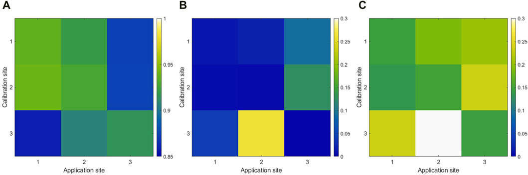
Figure 6. Portability of depth retrieval models developed via Optimal Band Ratio Analysis (OBRA) using data from a calibration site and then applied to a different site was quantified in terms of the (A) observed vs. predicted (OP) R², (B) normalized mean bias, and (C) normalized root mean squared error (RMSE).

The results of this analysis suggest that OBRA relations were highly portable across the three sub-reaches, with all possible combinations of calibration site and application site leading to OP R² > 0.85, with even better performance when an X vs. d relation established in AOI one was exported to AOI two or vice versa. Relatively low OP R² values occurred when a depth retrieval model from either AOI one or AOI two was applied in AOI three or when the model from AOI three was applied to AOI one. The diminished performance observed for these scenarios was a consequence of the much greater range of depths present in AOI three than in the other two sub-reaches, which led to the selection of a different, shorter-wavelength numerator band and a depth retrieval model that might have performed better in deeper water but also led to less reliable depth estimates in the relatively shallow areas that were more prevalent in AOIs one and two. For example, applying the OBRA relation calibrated in AOI three to AOI two led to a normalized bias approaching 30%, an order of magnitude greater than the small biases observed when OBRA was conducted on a per-AOI basis. Conversely, applying the X vs. d equations calibrated in AOIs one and two to AOI three led to relatively large, positive normalized biases, implying underprediction of depth in AOI three. Similarly, the discrepancy in the range of depths present in AOI three as compared to the other two sub-reaches also led to relatively low precision (i.e., larger normalized RMSE values represented by dark blue tones in Figure 6C) when the OBRA relation from AOI three was applied to the other two sub-reaches or when a depth retrieval model from AOI one or AOI two was used to predict depths in AOI three. In summary, our results suggest that relationships between depth and reflectance were highly portable among sub-reaches, but less so when the range of depths differed substantially between where a model is calibrated and where the model is then applied.

3.3 Comparison of sampling strategies for field data collection

In addition to transferring calibrated depth retrieval models among sub-reaches of the same river, another way to reduce the level of effort required to produce depth maps would be to decrease the number of field observations used in the calibration process. To assess the viability of this option, we evaluated whether field surveys that were progressively less dense than that we originally collected could still support UAS-based remote sensing of river bathymetry. Figure 4 illustrates all 32 sampling configurations we considered for AOI one, which range from the full data set of 1,262 points collected by wading and measuring cross sections and a longitudinal profile from a boat (configuration 1), to very sparse subsets thereof. For example, configuration 16 consisted of a single longitudinal profile and configuration 28 included only two of the original eight cross sections.

The results of this analysis are summarized in Figure 7, which shows how depth retrieval performance varied as a function of the field sampling strategy. Each column of this figure corresponds to one of the three depth retrieval performance metrics, OP R², normalized bias, and normalized RMSE. The top row presents results from sampling configurations that included the longitudinal profile (1–16) and the bottom row those that did not include the profile (17–32). Within each panel of Figure 7, the groups of bars represent different proportions of the total number of cross sections retained, either all eight cross sections for the leftmost group of bars, half (4), a quarter (2), or none of the cross sections. Finally, within each group of bars, the different colors represent different fractions of the available wading data retained, ranging from 100% (blue) to 50% (red), 25% (orange), and none (purple).

Figure 7

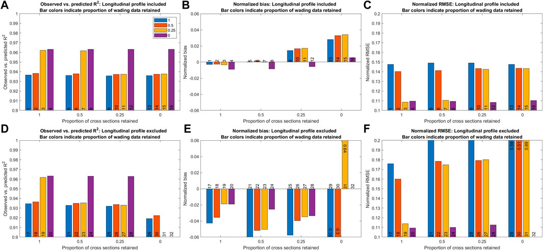
Figure 7. Summary of the analysis of the effects of different field sampling configurations on depth retrieval performance within area of interest (AOI one). The numbers at the base of each bar correspond to the sampling configurations illustrated in Figure 4. For configurations that led to performance metrics far outside the range of the others (29–32), the actual metric values are given at the top or bottom of the bars in (E) and (F). (A) Observed vs. predicted R²: Longitudinal profile included. Bar colors indicate proportion of wading data retained. (B) Normalized bias: Longitudinal profile included. Bar colors indicate proportion of wading data retained. (C) Normalized RMSE: Longitudinal profile included. Bar colors indicate proportion of wading data retained. (D) Observed vs. predicted R²: Longitudinal profile excluded. Bar colors indicate proportion of wading data retained. (E) Normalized bias: Longitudinal profile excluded. Bar colors indicate proportion of wading data retained. (F) Normalized RMSE: Longitudinal profile excluded. Bar colors indicate proportion of wading data retained.

The most salient result to emerge from this analysis is that for multispectral images acquired from a UAS along this sub-reach of the Sacramento River, the OBRA depth retrieval workflow was highly robust to the number and type of field data used for calibration. For example, for 28 of the 32 sampling configurations considered, OP R² values were greater than 0.93. Similarly, normalized bias was less than 4% in absolute value for any subset of the full survey that included the longitudinal profile and between 0% and -6% for any subset that did not include the profile but for which at least two cross sections were retained. Moreover, normalized RMSE was less than 15% for any subset of the full survey that included the longitudinal profile and less than 20% for any subset that did not include the profile, provided that two or more cross sections were used for calibration. The proportion of the available wading data used for calibration had very little impact on depth retrieval performance, even for the cases where no wading data were used. In fact, Figure 7 indicates that OP R² was higher and normalized RMSE was lower when wading measurements were not included in the calibration data set used as input to the OBRA algorithm. The only sampling configurations that led to unacceptably poor depth retrieval performance were the last four shown in Figure 4, when the longitudinal profile and all the cross sections were excluded, leaving only varying proportions of the wading data (configurations 29–31), as well as the trivial case of no data at all (configuration 32). This result was not surprising because relying entirely on shallow wading measurements would fail to capture the full range of depths present in the reach and so could not be expected to yield a depth retrieval model capable of performing well in deeper water not represented in the calibration data set. In contrast, the finding that robust depth retrieval models could be developed from very sparse field data sets was an unexpected but important result. For example, for a survey consisting of only two cross sections, with no wading measurements and no longitudinal profile (configuration 16), the OP R², normalized bias, and normalized RMSE were 0.96, 1%, and 11%, respectively. The results of this study indicate that the range of depths captured in the field data set used for calibrating image-derived depth estimates is more important than the number of observations used for this purpose.

To assess whether using such a low density of field data for calibration would compromise the portability of a depth retrieval model, we took the X vs. d relation for the OBRA based on only two cross sections in AOI one (sampling configuration 16) and applied it to the other two AOIs. The results of this analysis are summarized in Figure 8, which shows that exporting a version of Eq. 2 established using a very sparse field data set could yield reliable depth information in other, immediately adjacent sub-reaches of the same river. For example, the OP R² decreased only slightly from the value of 0.96 observed when the depth retrieval model was applied within AOI one to 0.95 and 0.92 when the model was applied to AOIs two and three, respectively. This slight reduction in performance was no more pronounced when using the much sparser field data set (configuration 16) than when all the field data were made available for calibration (configuration 1). The normalized bias shifted from slightly negative (−3%) when the model was applied internally to AOI one to positive when applied to the other two AOIs but remained small in absolute value, on the order of 3% or less. Similarly, the normalized RMSE increased from 11% to 12% and 16% when the model was applied to AOIs two and three, respectively, with the bigger increase for the latter AOI probably due to the greater depths present in the third sub-reach. In any case, these results imply that using a very sparse calibration data set from a single AOI would not compromise the portability of the resulting depth retrieval model to other sub-reaches of the same river.

Figure 8

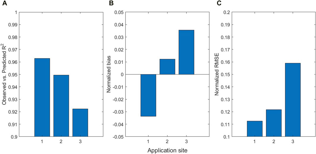
Figure 8. Assessment of the impact of exporting a depth retrieval model developed using a very sparse field data set from Area of Interest (AOI) one to the other two AOIs in terms of the (A) observed vs. predicted R², (B) normalized bias, and (C) normalized root mean squared error (RMSE).

To further substantiate this finding, we examined what might be considered the worst-case scenario: using data from only two cross sections in one sub-reach (AOI one) to calibrate an OBRA relation that was then applied to a nearby but not immediately adjacent sub-reach (AOI three) that also featured much greater depths (Figure 3; Table 1). Figure 9 summarizes our validation of the depth map for AOI three produced using the OBRA relation derived in AOI one on the basis of only two cross sections (sampling configuration 16). The histogram and summary statistics shown in Figure 9A indicate that image-derived depth estimates were biased shallow on average, with a mean error of 0.07 m, and reasonably precise, with an error standard deviation of 0.32 m. Of greater concern is the long tail of positive errors, with a maximum of 1.85 m, indicating large underpredictions of depth in many locations. The spatial pattern of these errors is illustrated in Figure 9B, where red tones highlight the inability of the depth retrieval model to capture the full depth of the pool along the outside of the bend throughout much of this sub-reach. The overall agreement in terms of the OP R² remains strong (0.92), but the discrepancy between the best-fit line and the one-to-one line of perfect agreement evident in Figure 9C indicates that depths tend to be over-predicted in water shallower than about 1.5 m and under-predicted in deeper water. This tendency is also manifested as an OP regression line with a negative, non-zero intercept and a slope greater than 1. These results were to be expected, given the much greater depths in AOI three than in AOI one, and a similar tendency to underpredict pool depth was observed even when using a depth retrieval model based on a full density field data set from AOI three. Rather than calling into question the portability of the depth retrieval model from AOI one, the results shown in Figure 9 reiterate the well-established, physics-based finding that passive optical approaches to depth retrieval are less reliable in deeper water and that relationships between depth and reflectance can saturate beyond a finite maximum detectable depth (Philpot, 1989).

Figure 9

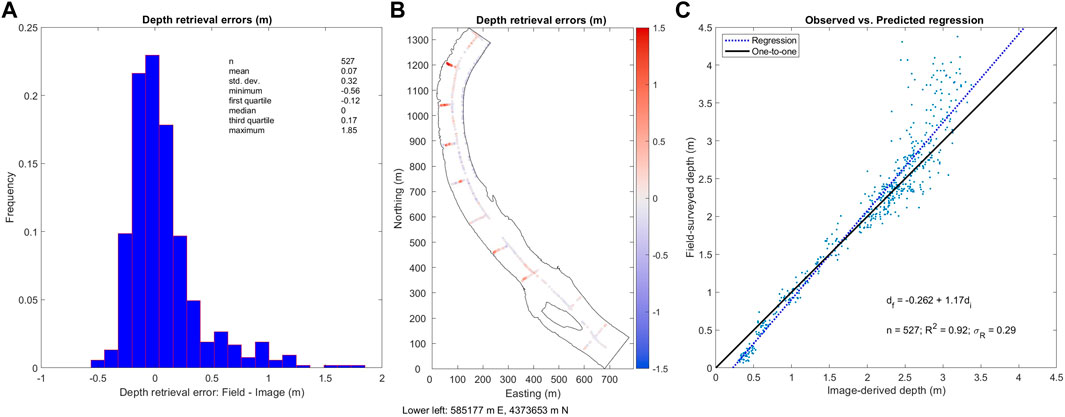
Figure 9. Validation of a bathymetric map produced for Area of Interest (AOI) three using a depth retrieval model created using a sparse field data set, consisting of only two cross sections, from AOI one. (A) Depth retrieval errors (m). (B) Depth retreival errors (m). (C) Observed vs. predicted regression.

4 Discussion

Spatially distributed information on water depth in river channels is critical for numerous applications in aquatic ecology, fluvial geomorphology, and river management. However, the difficulty and expense of acquiring such data via conventional field methods often limits the area for which detailed bathymetry is available, as well as the frequency with which these depth maps can be updated. Over the past couple of decades, remote sensing techniques have emerged as a viable alternative means of measuring river bathymetry more efficiently and over broader areas, with the capability of methods like OBRA to provide reliable depth estimates having been demonstrated across a range of fluvial environments. However, most previous studies were based on image data acquired from conventional aircraft or satellites, which are subject to various limitations in terms of spatial resolution, temporal frequency, and cost, as described in Section 1. This investigation, in contrast, focused on evaluating the feasibility of using UAS to map river bathymetry. UAS have become more widely available in recent years and provide an accessible means of obtaining higher resolution, less expensive images than can be acquired from aircraft or satellite platforms. An additional advantage of UAS is their ease of deployment, which facilitates agile, opportunistic response on an as-needed basis to examine a particular reach of interest, perhaps following a flood event that might lead to changes in channel morphology. This kind of efficiency also makes UAS-based data collection well-suited for more systematic, routine monitoring programs.

The results of this study provide strong evidence that UAS-based remote sensing is a viable approach to mapping river bathymetry, capable of providing accurate, precise depth estimates for reaches several km in length with relatively little effort. In this case, 3 days of image acquisition and field data collection were sufficient to produce a highly reliable depth map covering 4 km of the Sacramento River in northern California. These data were obtained using a commercially available vertical takeoff and landing UAS equipped with a standard, relatively inexpensive multispectral sensor and required only about 3 hours of actual flight time. The field crew consisted of a certified UAS pilot, a visual observer, a boat operator, and two hydrologic technicians for measuring depths by wading and with an echo sounder. After some initial image pre-processing, the main depth retrieval analysis was conducted within a freely available, standalone software package that makes the OBRA workflow accessible to end users without specialized training or computational resources. Moreover, we demonstrated that in addition to the standard, self-contained, per-image approach, a depth retrieval model developed for one sub-reach of a river could be exported to another, nearby area of interest and still yield reliable depth estimates. Similarly, we showed that the effort invested in collecting field data for calibration could be significantly reduced without compromising depth retrieval performance in either the sub-reach where the OBRA model was calibrated or other sub-reaches in close proximity. In aggregate, our findings imply that UAS-based remote sensing could yield bathymetric maps of river channels with a high degree of accuracy and precision at a reach scale of several km, even when only a sparse sample of field-based depth measurements is used for calibration and the resulting depth retrieval model is applied to a separate image from a distinct sub-reach. Based on the results of this study, we estimate that this approach could allow us to map approximately 5 km/day on a large, clear-flowing river like the Sacramento if we continue to prioritize image acquisition around solar noon, when the sun is highest in the sky and the amount of radiant energy incident upon the water surface is greatest. If we were to relax this constraint and acquire images across a broader range of times of day, this rate of mapping progress potentially could be doubled, but lower zenith angles would reduce signal-to-noise and could lead to more extensive shadowing by riparian vegetation.

While encouraging, these results are accompanied by some key caveats. Most importantly, as emphasized in Section 1, spectrally based depth retrieval is only feasible under a restricted set of environmental conditions that were satisfied for this section of the Sacramento River at low flow but which cannot be assumed in other places or at other times: clear water with minimal concentrations of suspended sediment, chlorophyll, or other optically significant constituents and relatively shallow depths on the order of 2–3 m. Again, turbid, deeper rivers are not conducive to this approach and applying OBRA, or any other method based on passive optical remote sensing, would be inappropriate. Further limitations of this study include its small spatial extent and the fact that the images were acquired on three consecutive days using a single sensor deployed from the same UAS platform. Although our portability analysis represented progress beyond the typical, per-image approach to depth retrieval, we considered only three AOIs that were located within 4 km of one another along the same river. Even at this level, ensuring consistent radiometric calibration across the three sites and dates was critical and points to the need to, at a minimum, process images to units of apparent surface reflectance prior to depth retrieval analysis. For low-altitude UAS operations, atmospheric effects can be considered less of a concern, but accounting for the influence of the atmosphere on the upwelling spectral radiance measured at the sensor could be much more important for higher-flying conventional aircraft and certainly for satellite platforms. Further research is thus needed to tackle the far greater challenges associated with upscaling this approach to much longer river segments, particularly if the data are acquired from different sensors and platforms and/or are separated from one another by greater periods of time. Enabling this kind of flexibility will require ensuring consistency among scenes by paying close attention to radiometric calibration and atmospheric correction. Similarly, careful sensitivity analyses must be conducted to quantify the effects of variations in water column optical properties and bottom reflectance, which could change significantly over longer river segments, particularly if tributaries enter and/or submerged aquatic vegetation becomes more extensive. Another important factor to consider is reflectance from the water surface due to sun glint, which could vary considerably over longer river segments where sensor view angles and solar azimuth relative to the orientation of the channel could change significantly (Legleiter et al., 2017).

Pursuing these larger-scale, longer-term objectives could more fully assess the potential of remote sensing for characterizing river systems. For the time being, however, the results of this study imply that a UAS-based approach could support highly efficient, operational bathymetric mapping. Moreover, the field data needed for calibration could be obtained with a minimal level of effort. For example, we found that surveying as little as two cross sections with an echo sounder provided sufficient data to establish a relationship between depth and reflectance that led to reliable depth estimates not only within the same sub-reach as the field survey but also in two nearby sub-reaches of the same river. While more data are always welcome, if for no other reason than to enable robust accuracy assessment, a hybrid field- and remote sensing-based approach might be more efficient. Rather than investing a lot of time and effort in collecting numerous cross sections, a longitudinal profile, and wading measurements, the calibration data required for OBRA could be obtained during a brief initial field campaign. The resulting depth maps could then be evaluated using a portion of the field data set aside for validation and used to identify deeper areas of the channel where image-derived depth estimates are least likely to be accurate. A follow-up field effort could then focus on filling in these pools with additional depth measurements, which might exceed the maximum detectable depth for the sensor deployed aboard the UAS, and addressing any other shortcomings identified in the remotely sensed bathymetry. This sort of targeted field data collection would be more efficient than the full, dense, uniform survey we conducted initially and thus more effectively take advantage of the capabilities of UAS-based remote sensing while also explicitly addressing the primary known deficiency of this approach: a tendency to underpredict depths in deeper water.

Data availability statement

The datasets presented in this study can be found in online repositories. The names of the repository/repositories and accession number(s) can be found below: The datasets generated and analyzed for this study can be found in the USGS ScienceBase catalog: Legleiter, C. J., and Harrison, L. R. (2023). Multispectral images and field measurements of water depth from the Sacramento River near Glenn, California, acquired September 14–16, 2021. U.S. Geological Survey Data Release, https://doi.org/10.5066/P9KEXVAR.

Author contributions

CL: Conceptualization, Data curation, Formal Analysis, Investigation, Methodology, Software, Validation, Visualization, Writing–original draft. LH: Conceptualization, Data curation, Funding acquisition, Investigation, Methodology, Project administration, Resources, Supervision, Validation, Writing–review and editing.

Funding

The author(s) declare financial support was received for the research, authorship, and/or publication of this article. This research was supported by awards from NOAA’s Uncrewed Systems Operations Center (UxSOC) and Uncrewed Systems Research Transition Office (UxSRTO).

Acknowledgments

Matt Pickett, Brian Taggart, Jason Woolard, Ben Taber, and Rafael Rodriguez assisted with field- and UAS-based data collection. We thank Greg Golet and Luis Ojeda of The Nature Conservancy for providing access to the Sacramento River at Hartley Island field site. Any use of trade, firm, or product names is for descriptive purposes only and does not imply endorsement by the U.S. Government.

Conflict of interest

The authors declare that the research was conducted in the absence of any commercial or financial relationships that could be construed as a potential conflict of interest.

Publisher’s note

All claims expressed in this article are solely those of the authors and do not necessarily represent those of their affiliated organizations, or those of the publisher, the editors and the reviewers. Any product that may be evaluated in this article, or claim that may be made by its manufacturer, is not guaranteed or endorsed by the publisher.

References

Agisoft (2023). MicaSense RedEdge MX processing workflow (including reflectance calibration) in agisoft metashape professional. Available at: https://agisoft.freshdesk.com/support/solutions/articles/31000148780-micasense-rededge-mx-processing-workflow-including-reflectance-calibration-in-agisoft-metashape-pro (Accessed August 25, 2023).

Google Scholar

Carbonneau, P., Fonstad, M. A., Marcus, W. A., and Dugdale, S. J. (2012). Making riverscapes real. Geomorphology 137, 74–86. doi:10.1016/j.geomorph.2010.09.030

CrossRef Full Text | Google Scholar

Dal Sasso, S. F., Pizarro, A., and Manfreda, S. (2021). Recent advancements and perspectives in UAS-based image velocimetry. Drones 5, 81. doi:10.3390/drones5030081

CrossRef Full Text | Google Scholar

Daniels, M. E., and Danner, E. M. (2020). The drivers of river temperatures below a large dam. Water Resour. Res. 56, e2019WR026751. doi:10.1029/2019wr026751

CrossRef Full Text | Google Scholar

Dilbone, E., Legleiter, C. J., Alexander, J. S., and McElroy, B. (2018). Spectrally based bathymetric mapping of a dynamic, sand-bedded channel: niobrara River, Nebraska, USA. River Res. Appl. 34, 430–441. doi:10.1002/rra.3270

CrossRef Full Text | Google Scholar

Dudley, P. N., John, S. N., Daniels, M. E., and Danner, E. M. (2022). Using decades of spawning data and hydraulic models to construct a temperature-dependent resource selection function for management of an endangered salmonid. Can. J. Fish. Aquatic Sci. 79, 73–81. doi:10.1139/cjfas-2021-0022

CrossRef Full Text | Google Scholar

Harrison, L. R., Legleiter, C. J., Overstreet, B. T., Bell, T. W., and Hannon, J. (2020). Assessing the potential for spectrally based remote sensing of salmon spawning locations. River Res. Appl. 36, 1618–1632. doi:10.1002/rra.3690

CrossRef Full Text | Google Scholar

Harrison, L. R., Legleiter, C. J., Sridharan, V. K., Dudley, P. N., and Daniels, M. E. (2022). Evaluating the sensitivity of multi-dimensional model predictions of salmon habitat to the source of remotely sensed River Bathymetry. Water Resour. Res. 58, e2022WR033097. doi:10.1029/2022WR033097

CrossRef Full Text | Google Scholar

Kwon, S., Gwon, Y., Kim, D., Seo, I. W., and You, H. (2023). Unsupervised classification of riverbed types for bathymetry mapping in shallow rivers using UAV-based hyperspectral imagery. Remote Sens. 15, 2803. doi:10.3390/rs15112803

CrossRef Full Text | Google Scholar

Legleiter, C. (2013). Mapping river depth from publicly available aerial images. River Res. Appl. 29, 760–780. doi:10.1002/rra.2560

CrossRef Full Text | Google Scholar

Legleiter, C., and Harrison, L. (2023). Multispectral images and field measurements of water depth from the Sacramento River near Glenn, California, acquired September 14-16, 2021. U.S. Geol. Surv. data release. doi:10.5066/P9KEXVAR

CrossRef Full Text | Google Scholar

Legleiter, C., and Harrison, L. R. (2019). Remote sensing of River Bathymetry: evaluating a range of sensors, platforms, and algorithms on the upper Sacramento River, California, USA. Water Resour. Res. 55, 2142–2169. doi:10.1029/2018WR023586

CrossRef Full Text | Google Scholar

Legleiter, C., Overstreet, B., and Kinzel, P. (2018). Sampling strategies to improve passive optical remote sensing of River Bathymetry. Remote Sens. 10, 935. doi:10.3390/rs10060935

CrossRef Full Text | Google Scholar

Legleiter, C., and Overstreet, B. T. (2012). Mapping gravel bed river bathymetry from space. J. Geophys. Res. - Earth Surf. 117, F04024. doi:10.1029/2012jf002539

CrossRef Full Text | Google Scholar

Legleiter, C., Roberts, D. A., and Lawrence, R. L. (2009). Spectrally based remote sensing of river bathymetry. Earth Surf. Process. Landforms 34, 1039–1059. doi:10.1002/esp.1787

CrossRef Full Text | Google Scholar

Legleiter, C. J. (2021). The optical river bathymetry toolkit. River Res. Appl. 37, 555–568. doi:10.1002/rra.3773

CrossRef Full Text | Google Scholar

Legleiter, C. J., Tedesco, M., Smith, L. C., Behar, A. E., and Overstreet, B. T. (2014). Mapping the bathymetry of supraglacial lakes and streams on the Greenland ice sheet using field measurements and high-resolution satellite images. Cryosphere 8, 215–228. doi:10.5194/tc-8-215-2014

CrossRef Full Text | Google Scholar

Legleiter, C. J. C., and Fosness, R. L. (2019). Defining the limits of spectrally based bathymetric mapping on a large river. Remote Sens. 11, 665. doi:10.3390/rs11060665

CrossRef Full Text | Google Scholar

Legleiter, C. J. C., Mobley, C. D., and Overstreet, B. T. (2017). A framework for modeling connections between hydraulics, water surface roughness, and surface reflectance in open channel flows. J. Geophys. Res. Earth Surf. 122, 1715–1741. doi:10.1002/2017jf004323

CrossRef Full Text | Google Scholar

Lyzenga, D. R. (1978). Passive remote-sensing techniques for mapping water depth and bottom features. Appl. Opt. 17, 379–383. doi:10.1364/AO.17.000379

PubMed Abstract | CrossRef Full Text | Google Scholar

Marcus, W. A., and Fonstad, M. A. (2010). Remote sensing of rivers: the emergence of a subdiscipline in the river sciences. Earth Surf. Process. Landforms 35, 1867–1872. doi:10.1002/esp.2094

CrossRef Full Text | Google Scholar

MicaSense (2023). How to use the calibrated reflectance panel (CRP). Available at: https://support.micasense.com/hc/en-us/articles/1500001975662-how-to-use-the-calibrated-reflectance-panel-crp- (Accessed August 25, 2023).

Google Scholar

Mobley, C. D. (1994). Light and water: radiative transfer in natural waters. San Diego: Academic Press.

Google Scholar

Mobley, C. D., Sundman, L. K., Davis, C. O., Bowles, J. H., Downes, T. V., Leathers, R. A., et al. (2005). Interpretation of hyperspectral remote-sensing imagery by spectrum matching and look-up tables. Appl. Opt. 44, 3576–3592. doi:10.1364/AO.44.003576

PubMed Abstract | CrossRef Full Text | Google Scholar

Moyle, P., Lusardi, R., Samuel, P., and Katz, J. (2017). State of the salmonids: status of California’s emblematic fishes 2017. Davis and California Trout, San Francisco, CA: Center for Watershed Sciences, University of California. Tech. rep.

Google Scholar

Niroumand-Jadidi, M., Bovolo, F., and Bruzzone, L. (2020). SMART-SDB: sample-specific multiple band ratio technique for satellite-derived bathymetry. Remote Sens. Environ. 251, 112091. doi:10.1016/j.rse.2020.112091

CrossRef Full Text | Google Scholar

Niroumand-Jadidi, M., Legleiter, C. J., and Bovolo, F. (2022). River bathymetry retrieval from landsat-9 images based on neural networks and comparison to SuperDove and sentinel-2. IEEE J. Sel. Top. Appl. Earth Observations Remote Sens. 15, 5250–5260. doi:10.1109/JSTARS.2022.3187179

CrossRef Full Text | Google Scholar

O’Sullivan, A. M., Wegscheider, B., Helminen, J., Cormier, J. G., Linnansaari, T., Wilson, D. A., et al. (2021). Catchment-scale, high-resolution, hydraulic models and habitat maps – a salmonid’s perspective. J. Ecohydraulics 6, 53–68. doi:10.1080/24705357.2020.1768600

CrossRef Full Text | Google Scholar

Philpot, W. D. (1989). Bathymetric mapping with passive multispectral imagery. Appl. Opt. 28, 1569–1578. doi:10.1364/AO.28.001569

PubMed Abstract | CrossRef Full Text | Google Scholar

Piégay, H., Arnaud, F., Belletti, B., Bertrand, M., Bizzi, S., Carbonneau, P., et al. (2020). Remotely sensed rivers in the Anthropocene: state of the art and prospects. Earth Surf. Process. Landforms 45, 157–188. doi:10.1002/esp.4787

CrossRef Full Text | Google Scholar

Pineiro, G., Perelman, S., Guerschman, J. P., Paruelo, J. M., Pi, G., Perelman, S., et al. (2008). How to evaluate models: observed vs. predicted or predicted vs observed? Ecol. Model. 216, 316–322. doi:10.1016/j.ecolmodel.2008.05.006

CrossRef Full Text | Google Scholar

Quantum Systems (2024). Discover QBase3D - the ultimate drone software solution , Available online: https://quantum–systems.com/qbase–3d/ (accessed 11 March 2024)

Google Scholar

Singer, M. B. (2008). Downstream patterns of bed material grain size in a large, lowland alluvial river subject to low sediment supply. Water Resour. Res. 44. doi:10.1029/2008WR007183

CrossRef Full Text | Google Scholar

Strelnikova, D., Perks, M. T., Dal Sasso, S. F., and Pizarro, A. (2023). “River flow monitoring with unmanned aerial system,” in Unmanned aerial systems for monitoring soil, vegetation, and riverine environments. Editors S. Manfreda,, and E. Ben Dor (Amsterdam, Netherlands: Elsevier), 231–269. doi:10.1016/B978-0-323-85283-8.00012-6

CrossRef Full Text | Google Scholar

Tomsett, C., and Leyland, J. (2019). Remote sensing of river corridors: a review of current trends and future directions. River Res. Appl. 35, 779–803. doi:10.1002/rra.3479

CrossRef Full Text | Google Scholar

U.S. Geological Survey (2023). USGS water data for the Nation. U.S. Geological Survey National Water Information System database.

Google Scholar

Winterbottom, S. J., and Gilvear, D. J. (1997). Quantification of channel bed morphology in gravel-bed rivers using airborne multispectral imagery and aerial photography. Regul. Rivers Res. Manag. 13, 489–499. doi:10.1002/(sici)1099-1646(199711/12)13:6<489::aid-rrr471>3.0.co;2-x

CrossRef Full Text | Google Scholar