Flow-induced buckling of elastic microfilaments with non-uniform bending stiffness

1 Introduction

Elastic filaments such as actin and microtubules serve as the backbone of cells by providing structural integrity to the intracellular matrix. Beyond this core function, fluid-structure interactions between these elastic fibers and their surrounding fluid are essential to many biological processes. One such example is cytoplasmic streaming, a process where motor protein movement in filament networks can drive fluid flow within cells (Verchot-Lubicz and Goldstein, 2010; Woodhouse and Goldstein, 2013; Suzuki et al., 2017). Advances in microfluidic methods and the rich non-linear dynamics that arise from the fluid-structure interactions have spurred many experimental, analytical and numerical investigations into the elastohydrodynamics of single filament systems (Wiggins et al., 1998; Chelakkot et al., 2010; Chelakkot et al., 2012; Kantsler and Goldstein, 2012; Harasim et al., 2013; Chakrabarti et al., 2020a; Chakrabarti et al., 2020b).

Like the deformation of Euler beams, elastic filaments moving freely in viscous fluids can undergo a buckling instability if the compressive forces acting upon the filament exceed the internal restorative elastic forces. This phenomenon has been well characterized in cellular (Young and Shelley, 2007; Wandersman et al., 2010; Quennouz et al., 2015), extensional (Kantsler and Goldstein, 2012; Manikantan and Saintillan, 2015), shear (Becker and Shelley, 2001; Liu et al., 2018), and other flow profiles (Chakrabarti et al., 2020a; Chakrabarti et al., 2020b). Thermal fluctuations due to Brownian motion add additional subtleties to this elastohydrodynamic problem: experiments have demonstrated the rounding of this buckling instability (Kantsler and Goldstein, 2012), which has been analytically substantiated as well (Baczynski et al., 2008; Manikantan and Saintillan, 2015). This well-characterized instability is crucial in dictating the transport of these filaments. Bending and buckling allows fibers to move as random walkers near hyperbolic stagnation points in a 2D cellular flow array (Young and Shelley, 2007), whereas thermal fluctuations hinder the transport of these fibers and trap them within the vortical cells (Manikantan and Saintillan, 2013). More recently, filaments have been shown to be trapped around circular objects due to flow-induced buckling (Chakrabarti et al., 2020b).

However, in all of these studies, the bending stiffness or rigidity of the filament backbone is assumed to be uniform. This may not hold true in many physical systems. For example, protein adsorption onto filaments can be highly non-uniform, following heterogeneous condensation that has been linked to the Rayleigh-Plateau instability (Hernández-Vega et al., 2017; Setru et al., 2021). This non-uniformity has been characterized in recent experiments that correlate regions of increased microtubular bending with enhanced protein adsorption (Tan et al., 2019). Another example involves chromatin fibers with highly non-uniform bending-stiffness profiles that display anomalous segregation and depletion, playing a crucial role in genome organization inside eukaryotic cells (Girard et al., 2020). Some past studies have modeled filaments with heterogeneous mechanical properties and predicted their resulting deformation and fragmentation behavior (De La Cruz et al., 2015; Lorenzo et al., 2020), but it is unclear what shapes and configurations these filaments can assume. A platform to predict the expected filament shapes and buckling thresholds of non-uniformly stiff filaments in fluid flow has not yet been established. Moreoever, a quantitative analysis of the growth of buckling modes is still missing. In this work, we present results from linear stability analysis and non-linear simulations for heterogeneously stiff filaments undergoing the buckling instability in flow.

In what follows, we provide a mathematical description of filaments with non-uniform and heterogeneous rigidity profiles coupled to slender-body theory for viscous flows. In addition to a constant bending rigidity traditionally used in conjunction with slender-body theory, we analyze two examples of asymmetrical rigidity profiles with analytical forms motivated by protein attachment/detachment onto/from filaments. We also lay out the process to determine fundamental modes or shapes for any rigidity profile, and provide a consistent framework to extract amplitudes of these modes from future simulations and experiments. We use this platform to report qualitative and quantitative differences in linear stability analyses and non-linear Brownian simulations across select non-uniform stiffness profiles.

2 Problem description

Describing the dynamic conformations of flexible filaments in flow requires solving the Navier-Stokes equation coupled to elastic equations for the filament backbone. The length and time scales are such that the Navier-Stokes equation reduces to the Stokes equation: classic works on slender-body theory for low-Reynolds-number hydrodynamics then describe the fluid dynamics of the problem if the force distribution corresponding to the presence of a filament are known (Batchelor, 1970a; Keller and Rubinow, 1976; Johnson, 1980). For this work, we will use the local Brownian motion variation of slender-body theory to couple microfilament dynamics with a viscous fluid (Tornberg and Shelley, 2004; Manikantan and Saintillan, 2013; Manikantan and Saintillan, 2015). This variation accounts for the anisotropy of the filament based on its shape and orientation, but neglects non-local hydrodynamic interactions between different points on the filament.

2.1 Energy functional and force balance

We will consider an inextensible elastic filament of characteristic thickness 2a and length L which is parameterized by arclength s. Here, s is a material parameter for the filament that serves to discretize the filament backbone from −L/2 to L/2 and thus is independent of time t. The slenderness of the filament is captured by the slenderness ratio ɛ = a/L ≪ 1. The centerline coordinates of the filament are x(s, t) = (x (s, t), y(s, t), z(s, t)); for the purposes of this work, we shall consider flow and buckling in the 2D x–y plane. When a non-Brownian filament is placed in flow, the competition between the external viscous forces and internal elastic or tensile forces describes its dynamics. We follow the approach used by Li et al. (2013) to derive a non-uniform force across such a filament, starting with the energy functional:

$\mathcal{E}=\frac{1}{2}{\int }_{L/2}^{-L/2}\left(\kappa \left(s\right){\mathbf{x}}_{ss}^2+T\left(s\right)\left({\mathbf{x}}_s\cdot {\mathbf{x}}_s-1\right)\right)ds-{\int }_{L/2}^{-L/2}\mathbf{f}\left(s\right)\cdot \mathbf{x}\left(s\right)ds.(1)$

Here, κ(s) is the non-uniform stiffness or bending modulus of the filament (κ(s) = E(s)I where E(s) is Young’s Modulus and I = πa⁴/4 is the second moment of inertia of a rod), x_ss is the filament curvature, T represents the line tension experienced by the filament which enters as a Lagrange multiplier, and f is the force per unit length exerted on the filament by the fluid. All subscripts on variables represent partial derivatives with respect to the subscript unless otherwise stated.

Physically, the terms in the first integral of Eq. 1 corresponds to an energetic penalty for bending and stretching, respectively. The last integral term relates the energy to the force at a particular location on the filament. To obtain this force, we can take variational derivatives of the energy functional above via the Euler-Lagrange Equation:

$\frac{\partial \mathcal{E}}{\partial \mathbf{x}}-\frac{\partial }{\partial s}\left(\frac{\partial \mathcal{E}}{\partial {\mathbf{x}}_s}\right)+\frac{{\partial }^2}{\partial s^2}\left(\frac{\partial \mathcal{E}}{\partial {\mathbf{x}}_{ss}}\right)=0.(2)$

This gives the dimensional force acting on the filament in the absence of Brownian motion:

$\mathbf{f}\left(s\right)=-{\left(T\left(s\right){\mathbf{x}}_s\right)}_s+{\left(\kappa \left(s\right){\mathbf{x}}_{ss}\right)}_{ss}.(3)$

2.2 Constitutive equations of motion

The filament is immersed in a fluid of viscosity μ with an imposed velocity field U₀(x(s, t), t). The velocity of the filament is then approximated by the local version of the slender-body theory centerline equation (Batchelor, 1970a; Keller and Rubinow, 1976; Johnson, 1980; Tornberg and Shelley, 2004; Manikantan and Saintillan, 2013; Manikantan and Saintillan, 2015; Chakrabarti et al., 2020b):

$8\pi \mu \left({\mathbf{x}}_t\left(s,t\right)-{\mathbf{U}}_0\left(\mathbf{x},t\right)\right)=-\mathbf{\Lambda }\left[\mathbf{f}\right].(4)$

Here, x_t is the time derivative of the filament centerline, Λ is a local operator that captures the filament’s anisotropic interaction with the surrounding fluid, and f is the force per unit length acting on the filament as given by Eq. 3. The local operator is given by

$\mathbf{\Lambda }[\mathbf{f}]\left(s\right)=\left(\left(c+1\right)\mathbf{I}+\left(c-3\right){\mathbf{x}}_s{\mathbf{x}}_s\right)\cdot \mathbf{f},(5)$

where x_sx_s is the dyadic product of the unit vectors x_s(s) that are locally tangent to the filament centerline and c = ln(1/ɛ²).

In the absence of Brownian motion, we non-dimensionalize Eqs. 3, 4 with length scales over L, time with the fluid flow strength $\dot{\gamma }$, and forces with a characteristic elastic force κ/L². These quantities collect into a single dimensionless parameter:

$\bar{\mu }=\frac{8\pi \mu \dot{\gamma }{L}^2}{\kappa /L^2},(6)$

which can be interpreted as the ratio of viscous forces to elastic forces. Non-dimensionalization of Eqs. 3, 4 respectively results in the following dimensionless centerline velocity and force expressions.

$\bar{\mu }\left({\mathbf{x}}_t\left(s,t\right)-{\mathbf{U}}_0\left(\mathbf{x}\left(s\right),t\right)\right)=-\mathbf{\Lambda }\left[\mathbf{f}\right],(7)$

$\mathbf{f}\left(s\right)=-{\left(T{\mathbf{x}}_s\right)}_s+{\left(B\left(s\right){\mathbf{x}}_{ss}\right)}_{ss},(8)$

Where B(s) is now the dimensionless stiffness profile across the filament. All variables hereafter are assumed to be dimensionless unless otherwise stated.

2.3 Biologically motivated stiffness profiles

Protein attachment onto microtubules and other elastic filaments can be highly non-uniform (Hernández-Vega et al., 2017; Tan et al., 2019; Setru et al., 2021), resulting in heterogeneous structural properties. We are interested in the stability and configurations of filaments with non-uniform stiffness, which could shed light into their transport across streamlines and in complex flows. Motivated by protein adsorption or desorption that locally strengthens or weakens the filament backbone, we use the following analytical forms of bending stiffness profiles (Figure 1).

$B_1\left(s\right)=1,(9)$

$B_2\left(s\right)=1-\frac{1}{2}{e}^{-100{\left(s+\frac{1}{4}\right)}^2},(10)$

$B_3\left(s\right)=2+\text{erf}\left(10s\right).(11)$

FIGURE 1

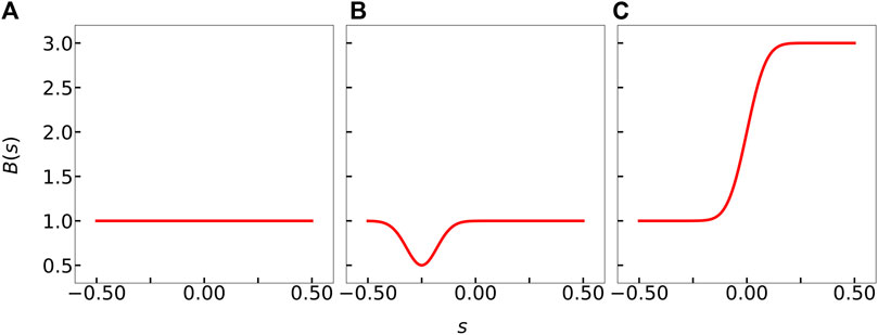
FIGURE 1. Rigidity profiles examined in this work. (A) Constant rigidity B₁(s). (B) Locally weak stiffness profile B₂(s) to reflect structural degradation due to protein attachment. (C) Asymmetrically rigid stiffness profile B₃(s) to reflect higher resistance to bending due to selective protein attachment one-half of the filament.

The constant stiffness profile B₁(s) is traditionally used by slender-body theory calculations, and we use this to test our predictions against previous works (Manikantan and Saintillan, 2015; Chakrabarti et al., 2020a). The asymmetrical stiffness profiles B₂(s) and B₃(s) reflect potential protein adsorption patterns that locally modifies filament’s stiffness. B₂(s) was chosen to model the potential stiffness profile for a locally weak and asymmetric backbone that results in the “fish hook”-like microtubule in Tan et al. (2019)’s study. B₃(s), on the other hand, may represent a situation where one-half of a microtubule is weakened (or, equivalently, stiffened) due to protein condensation. Note, however, that the framework we develop below works for any fitted or modeled form of B(s): the choices in Eqs. 9–11 are merely illustrative examples that we use to demonstrate our methods.

2.4 Brownian motion

Microscopic objects suspended in a fluid medium are subjected to Brownian forces: these thermal fluctuations are characterized by k_BT where k_B is Boltzmann’s constant and T is the absolute temperature. The elastic resistance of elongated structures to bending due to fluctuations is characterized by the persistence length ℓ_p = κ/k_BT. Alternatively, ℓ_p a measure of distance between two points on an object at which the local tangent vectors become uncorrelated due to thermal fluctuations. Microtubules have a persistence length of approximately 5 mm (Gittes et al., 1993), which is roughly $\mathcal{O}(100-1000)$ times larger than their typical lengths. Actin filaments are more easily deformed by Brownian fluctuations, with ${\ell }_p/L=\mathcal{O}(1-10)$ (Gittes et al., 1993).

The stochastic Brownian force enters as an additional term in the dimensional force expression in Eq. 3:

$\mathbf{f}\left(s\right)=-{\left(T\left(s\right){\mathbf{x}}_s\right)}_s+{\left(\kappa \left(s\right){\mathbf{x}}_{ss}\right)}_{ss}+{\mathbf{f}}^{Br}\left(s,t\right).(12)$

We set up Brownian forces f^Br to satisfy the fluctuation-dissipation theorem of statistical mechanics that describes a fluctuating force with zero mean and finite variance proportional to k_BT and the hydrodynamic resistance:

$⟨{\mathbf{f}}^{Br}\left(s,t\right)⟩=0,(13)$

$⟨{\mathbf{f}}^{Br}\left(s,t\right){\mathbf{f}}^{Br}\left(s^{\prime },t^{\prime }\right)⟩=2k_{B}T{\mathbf{M}}^{-1}\delta \left(s-s^{\prime }\right)\delta \left(t-t^{\prime }\right).(14)$

Here, ⟨⟩ represents an ensemble average, δ is the dirac delta function, and M is the dimensional mobility tensor (8πμ)⁻¹ ((c+1)I+(c−3)x_sx_s) from Eq. 5. Non-dimensionalizing Eqs. 4, 12 now requires recognizing the large scale separation between the flow and Brownian time scales (Munk et al., 2006; Manikantan and Saintillan, 2013; Manikantan and Saintillan, 2015). To accommodate filament deflections at these Brownian time scales, we use the relaxation time of the elastic filament 8πμL⁴/κ to non-dimensionalize time scales associated with filament movement. The external flow field is still scaled over $L\dot{\gamma }$, and lengths and forces are non-dimensionalized like before. The resulting dimensionless constitutive equations for Brownian motion are then.

${\mathbf{x}}_t\left(s,t\right)-\bar{\mu }{\mathbf{U}}_0\left(\mathbf{x}\left(s\right),t\right)=-\mathbf{\Lambda }\left[\mathbf{f}\right],(15)$

$\mathbf{f}\left(s\right)=-{\left(T{\mathbf{x}}_s\right)}_s+{\left(B\left(s\right){\mathbf{x}}_{ss}\right)}_{ss}+\sqrt{\frac{L}{{\ell }_p}}\mathit{\xi }\left(s\right).(16)$

Where ξ(s) is the dimensionless Brownian force.

2.5 Computational methods

We employ numerical methods that have been previously described in detail and tested across various flow geometries (Tornberg and Shelley, 2004; Manikantan and Saintillan, 2013; Manikantan and Saintillan, 2015; Chakrabarti et al., 2020b). Briefly, Eqs. 7, 15 contain an unknown line tension that is first determined by applying the identity ${({\mathbf{x}}_s\cdot {\mathbf{x}}_s)}_t=0$. The resulting differential equation in T(s) is solved using tension-free boundary conditions: T|_s=±1/2 = 0. Then, the filament position is solved with the torque-free and force-free boundary conditions (Landau and Lifshitz, 1986):

$B\left(s\right){\mathbf{x}}_{ss}{|}_{s=-\frac{1}{2}}=B\left(s\right){\mathbf{x}}_{ss}{|}_{s=+\frac{1}{2}}=0,(17)$

${\left(B\left(s\right){\mathbf{x}}_{ss}\right)}_s{\mid }_{s=-\frac{1}{2}}={\left(B\left(s\right){\mathbf{x}}_{ss}\right)}_s{\mid }_{s=+\frac{1}{2}}=0.(18)$

All spatial and time derivatives are approximated with second-order finite difference approximations (Tornberg and Shelley, 2004). However, the fourth derivative term in the elastic term in the expression for the force exerted on the filament enforces a stringent restriction on the time step size. This problem is mitigated with a semi-implicit time marching scheme previously developed by Tornberg and Shelley (2004). The work presented here uses a slenderness ratio ɛ of 0.01.

Brownian forces are calculated from Eq. 16 using previously established methods (Manikantan and Saintillan, 2013; Manikantan, 2015). We numerically evaluate ξ(s) as:

$\mathit{\xi }\left(s\right)=\sqrt{\frac{2}{\mathrm{\Delta }s\mathrm{\Delta }t}}\mathbf{B}\cdot \mathit{\omega }.(19)$

Here, ω is a random vector from a Gaussian distribution of zero mean and unit variance, Δs is the grid spacing of the filament, Δt is the time step size, and B is the tensor square root of M⁻¹ such that B ⋅B^T = M⁻¹. We verify our results with the uniform stiffness profile against established past works involving non-Brownian (Tornberg and Shelley, 2004) as well as Brownian (Manikantan and Saintillan, 2015) filaments in shear flow.

3 Results

We will first present our numerical results of non-linear simulations of a non-Brownian fiber. We then use linear stability analysis to help explain our numerical findings and establish key differences between the stiffness profiles. Following this, we compare our linear mode predictions from stability analyses with the filament shapes observed at the onset of instability in non-linear and Brownian simulations.

3.1 Simulation results

We begin by describing our observations from non-Brownian simulations of a filament with the three different bending stiffness profiles shown in Figure 1. We initially orient a filament along a straight line at an angle of θ = 8π/9 relative to the horizontal and supply a perturbation of magnitude $\mathcal{O}(10^{-4})$ to the filament’s y-component to induce buckling in shear flow U₀ = (y, 0) (Figure 2A). In this configuration, the filament is placed in the compressive quadrants of shear flow, coinciding with a negative parabolic filament tension (Figure 2B). As the filament rotates, the compressive forces acting upon the filament eventually overcome the internal elastic resistance to bending, causing the filament to buckle. During this process, the filament tension loses its parabolic profile. Once the filament is in the extensional quadrants, the internal filament tension is positive and stretches the filament: the rightmost panels in Figure 2 show the configuration at θ = π/9, approximately at t = 5.464. This behavior in shear flow has been well studied and documented for a constant stiffness profile (Tornberg and Shelley, 2004). We observe qualitative differences between the filament configuration and tension by comparing the case of constant stiffness with the locally weak stiffness profile B₂(s) and the asymmetrically rigid stiffness profile B₃(s): As expected, the magnitude of tension fluctuations and deformations are larger for the locally weak profile.

FIGURE 2

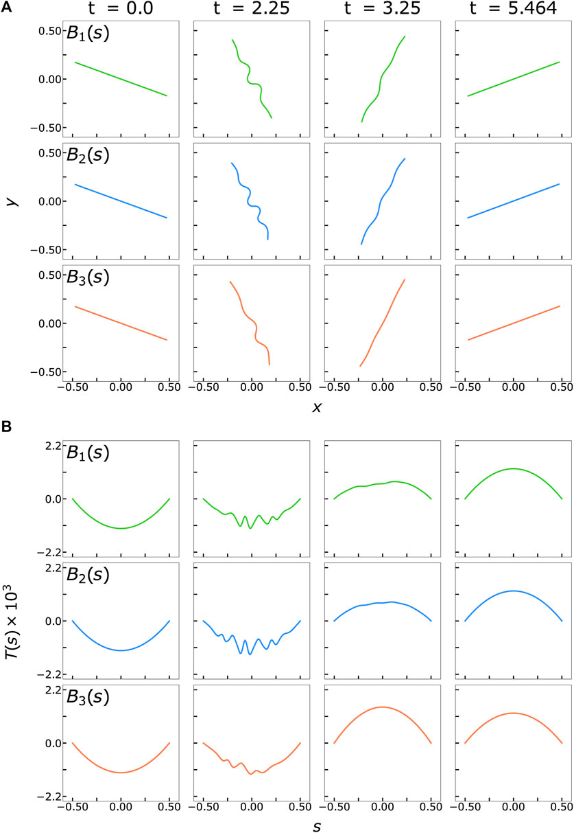
FIGURE 2. (A) Snapshots of filament buckling behavior in non-Brownian shear flow at various time points based on the three different rigidity profiles, all for flow strength $\bar{\mu }=5\times 10^5$ (B) The filament tension profile at the same timepoints as a function of the arclength s.

These differences among the stiffness profiles can be better quantified by comparing the effective compression or the filament end-to-end length deficit in Figure 3A. This quantity is defined as $L_{ee}^{*}=1-L_{ee}/L$, where L_ee is the end-to-end distance. A locally weak filament is more compressed relative to a uniformly stiff filament, whereas the asymmetrically stiffer filament is more resistant to end-to-end compression. The same trends can be quantified by comparing the filament elastic energy $E_{\mathit{elastic}}=1/2{\int }_{-L/2}^{L/2}B(s){\mathbf{x}}_{ss}^{2}ds$. We observe that the filament compression trends are analogous to the trends in elastic energy in Figure 3B.

FIGURE 3

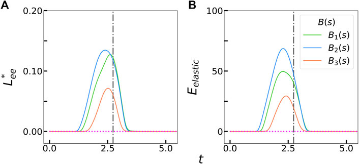
FIGURE 3. (A) Measured filament compression $L_{ee}^{*}$ and (B) elastic energy for the duration of the simulation of the three stiffness profiles in Figure 2. The magenta dotted line in each panel represents a rigid, unperturbed filament. The gray dash-dot vertical line represents the time at which a rigid filament is oriented at θ = π/2 relative to the horizontal.

These deformations and storage or dissipation of elastic energy introduces rheological signatures in the suspended fluid (Batchelor, 1970b; Tornberg and Shelley, 2004; Chakrabarti et al., 2021). To quantify the effects of these different stiffness profiles on the stress system of the fluid containing the filament, we calculate the particle extra stress tensor (Batchelor, 1970b):

$\mathit{\sigma }=\frac{1}{2}{\int }_{-L/2}^{L/2}\left[\mathbf{f}\left(s\right)\mathbf{x}\left(s\right)+\mathbf{x}\left(s\right)\mathbf{f}\left(s\right)\right]ds.(20)$

We show the evolution of the first and second normal stress differences, N₁ = σ_xx−σ_yy and N₂ = σ_yy−σ_zz respectively, in Figures 4A, B. The first normal stress difference is zero for a rigid rod rotating in shear flow and non-zero for buckled filaments over a full rotation. (Becker and Shelley, 2001; Tornberg and Shelley, 2004; Chakrabarti et al., 2021) To confirm this, we quantify the total extra stress during a full deformation cycle by integrating the area under the curves from t = 0 to t = 5.464, such that the filament is approximately oriented at π/2 from the horizontal halfway through this period (Table 1). We obtain a small but negative value for N_1,tot for a rigid rod (dotted pink line in Figure 4A). This could be attributed to our chosen initial filament orientation, choice of parameters, or absence of the non-local operator in Eqs. 7, 8. Nonetheless, a buckled filament with a uniform stiffness profile yields a positive non-zero first normal stress difference, in agreement with previous studies. (Becker and Shelley, 2001; Tornberg and Shelley, 2004; Chakrabarti et al., 2021) Interestingly, N_1,tot for a locally weak B₂(s) stiffness profile is larger than that for a uniformly stiff filament. In a confined flow geometry where the fluid is entrapped between walls, this corresponds to the fluid exerting more stress on the walls. N_1,tot for a asymmetrically rigid B₃(s) stiffness profile is also positive and non-zero, but smaller in magnitude than the other stiffness profiles. These results suggest that the extent of filament buckling is correlated with the magnitude of the first normal stress difference. Modifying the filament stiffness profile to favor buckling deformations will increase N_1,tot. The N_2,tot trends are analogous to those of N_1,tot, where the total stress difference is the highest for a locally weak filament backbone.

FIGURE 4

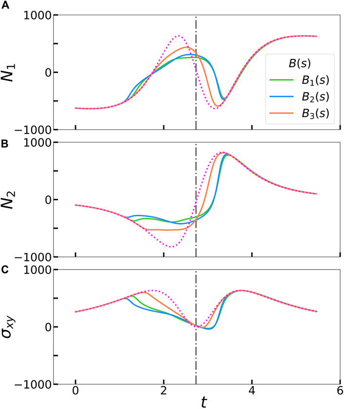
FIGURE 4. Calculated partcle extra stress contributions for the three different rigidity profiles during from Figure 2: (A) First normal stress difference N₁, (B) second normal stress difference N₁, and (C) shear stress σ_xy. The magenta dotted line in each panel represents an unperturbed filament that rotates as a rigid rod. The gray dash-dot vertical line represents the time at which a rigid rod is oriented at θ = π/2 relative to the horizontal.

TABLE 1

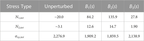
TABLE 1. Total value of stress types by integration of area under the curve in Figure 4 for each stiffness profile. The unperturbed column represents a filament without a supplied perturbation so it rotates like a rigid rod in shear flow (corresponding to the dotted magenta lines in Figure 4.

Plotting the evolution of shear stresses, σ_xy, over the duration of the simulation also reveals differences between the three stiffness profiles in Figure 4C. Tornberg and Shelley (2004) reported that filament buckling reduces the shear stress in comparison to a rigid, unbuckled filament. Excess local buckling, associated with a higher end-to-end length deficit and elastic energy in our simulations, could further reduce the shear stress perceived by the filament. To confirm this, we compute the total shear stress for each stiffness profile during the same time period as for the stress differences and report the values in Table 1. With our chosen stiffness profiles, more buckling is correlated with lower shear stress.

3.2 Linear stability analysis

To help explain these observed differences from our simulations, we turn our attention to linear stability analysis for a heterogeneously stiff filament in extensional flow; we expect quantitative features from such an analysis to carry over to shear flow which is combination of extension and rotation. An unperturbed filament resting in along the x-axis of a 2D extensional flow profile of U₀ = (−x, y) adopts an unperturbed parabolic tension profile of the form $T(s)=\bar{\mu }(1/4-s^2)/4c$ (Batchelor, 1970a; Kantsler and Goldstein, 2012). We define the unperturbed configuration of the filament as x(s, t) = (s, 0). Acknowledging that c ≫ 1 for slender fibers where c = ln (ɛ²e), we simplify Eq. 7 as

$\bar{\mu }\left({\mathbf{x}}_t-{\mathbf{U}}_0\right)=c\left(\mathbf{I}+{\mathbf{x}}_s{\mathbf{x}}_s\right)\cdot \mathbf{f}.(21)$

Perturbing Eq. 21 with small vertical displacement h(s, t) and neglecting higher order terms yields a linearized equation for perturbations:

$\bar{\mu }\left(h_t-h\right)=c\left(-2T_s{h}_s-T{h}_{ss}+B_{ss}{h}_{ss}+2B_s{h}_{\mathit{sss}}+B\left(s\right)h_{\mathit{ssss}}\right).(22)$

In contrast with previous linear stability analyses, Eq. 22 accounts for any modeled or fitted stiffness profile B(s). We perform a normal mode analysis by setting $h(s,t)=\widehat{h}(s)e^{\sigma t}$ where $\widehat{h}(s)$ is the mode shape and σ is the associated complex growth rate. Substituting the normal modes into Eq. 22 yields the an eigenvalue-eigenfunction (growth rate and mode shapes, respectively) problem:

$\begin{array}{c}\hfill B\left(s\right)\frac{{\partial }^4\widehat{h}}{\partial s^4}+2B_s\frac{{\partial }^3\widehat{h}}{\partial s^3}+\left(B_{ss}-\frac{\bar{\mu }}{4c}\left[\frac{1}{4}-s^2\right]\right)\frac{{\partial }^2\widehat{h}}{\partial s^2}+\frac{\bar{\mu }s}{c}\frac{\partial \widehat{h}}{\partial s}-\frac{\bar{\mu }}{c}\left(\sigma -1\right)\widehat{h}=0.\end{array}(23)$

This problem is numerically solved by applying the torque-free and force-free boundary conditions of Eqs. 17, 18. Like our simulations, we approximate the derivatives with second-order finite differences. The eigenspectrum maps in Figure 5 plot the real component of the growth rate σ as a function of the flow strength $\bar{\mu }$ to describe the stability of mode shapes for each stiffness profile. We define the mode number of the filament shapes realized in our analysis as the number of inflections in the mode shape at the onset of instability and track them over a range of $\bar{\mu }$ values, but these patterns can drastically change, as we illustrate below.

FIGURE 5

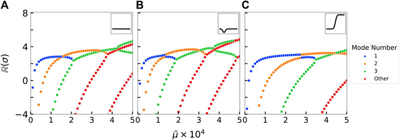
FIGURE 5. Eigenspectrum stability maps for three different rigidity profiles that highlight the stability of each mode as a function of the elastoviscous number $\bar{\mu }$. (A) is constant rigidity B₁(s), (B) is locally weak stiffness profile B₂(s), and (C) is asymmetrically rigid stiffness profile B₃(s). Positive growth rates $(\mathbb{R}(\sigma )>0)$ correspond to unstable modes. Modes are color-coded based on their mode number with “Other Mode Number” indicating fourth and higher modes. Data plotted on the graphs are plotted in increments of 1,000 $\bar{\mu }$. Insets show stiffness profiles corresponding to each eigenspectrum map.

In the case of a uniform stiffness profile, plotting the growth rate as a function of the flow strength reveals a familiar and well-studied landscape (Young and Shelley, 2007; Guglielmini et al., 2012): increasing the flow strength sequentially destabilizes higher buckling modes. The first mode is typically “U” shaped and appears at the threshold $\bar{\mu }\approx \mathrm{1,258}$ (Table 2). This onset of instability is consistent with previous findings (Young and Shelley, 2007; Guglielmini et al., 2012; Kantsler and Goldstein, 2012; Chakrabarti et al., 2020a). Increasing $\bar{\mu }$ to approximately 6,358 destabilizes the second mode, typically “S” shaped. The third mode, typically “W” shaped, becomes unstable at $\bar{\mu }\approx \mathrm{15,850}$. The stability curves for odd-numbered modes (first mode, third mode, etc.) have a tendency to merge with each other, physically corresponding to an additional “bump” appearing in the shape. For instance, the “U” shape develops a bump in the center around the merger with the “W” shape; likewise, even-numbered modes merge with each other (Figure 5A). When these merger events happen, we label the resulting shape with the higher numbered mode.

TABLE 2

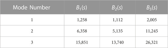
TABLE 2. Critical flow strengths representing the onset of instability (σ =0) for the first three modes for each rigidity profile.

The non-uniform filament stiffness profiles lead to noticeable changes in their respective eigenspectrum maps. The locally weak B₂(s) stiffness profile is characterized by a decrease in the rigidity on one side of the filament, potentially decreasing the overall stability of the filament. On the other hand, the asymetrically rigid B₃(s) stiffness profile is characterized by a rapid increase in the rigidity on one side of the filament, potentially strengthening the filament against buckling. Such changes to the stiffness profiles result in an earlier or delayed onset of instability of the buckling modes as shown in Table 2, confirming our initial hypotheses about filament stability.

To examine the evolution of the predicted mode shapes between the different stiffness profiles, we compare $\widehat{h}(s)$ for each stiffness profile at various $\bar{\mu }$ values. Examining the first mode shape at its onset of instability reveals minute differences in the shape between the different stiffness profiles (Figure 6A). However, we start to see differences in the shape of the first mode and visible effects of asymmetry upon increasing the flow strength significantly beyond the critical $\bar{\mu }$ corresponding to that mode (Figure 6B). Similarly, comparing the third mode (Figures 6C, D), we see that the difference in stiffness profiles results in minute differences near critical thresholds, whereas ramping up the flow strength reveals dramatic changes and asymmetries in the mode shape.

FIGURE 6

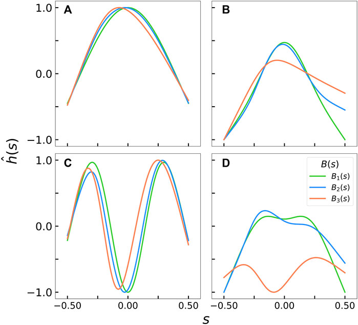
FIGURE 6. Comparison of the first and third mode shapes for each rigidity profile at various $\bar{\mu }$ values. (A) and (C): The first and third mode shapes at the onset of instability, respectively (see Table 2 for critical $\bar{\mu }$ values). (B) and (D): The first and third mode shapes at flow strengths much larger than these critical values, at $\bar{\mu }=\mathrm{18,000}$ and at $\bar{\mu }=\mathrm{30,000}$ respectively. All mode shapes are normalized to a max amplitude of 1.

For all the discussion so far, we must note that linear stability analysis predicts the most dominant mode shapes and mode numbers at specific $\bar{\mu }$ values in a deterministic simulation. The non-linear shapes seen in the simulations, however, depend on the perturbations applied to the filament. In particular, real microfilaments are subject to Brownian fluctuations and so we can at best make statistically expected predictions of buckling shapes or thresholds. Indeed, Brownian fluctuations are a source of constant perturbations and excite all modes equally (Kantsler and Goldstein, 2012), although excited modes are expected to be consistent with the deterministic predictions (Manikantan and Saintillan, 2015). In what follows, we develop a framework to address stochastic buckling of Brownian microfilaments and to quantify the role of thermal fluctuations and non-uniform rigidity on the statistically expected stability and shape.

3.3 Comparison of simulations with stability analysis

We will compare the predictions of the stability analyses with filament shapes that emerge in non-linear and Brownian simulations at short times. As an illustration, we perform Brownian ensemble simulations (statistical averages across 200 simulations for each data point) for a moderately rigid filament (ℓ_p/L = 100) with the three different stiffness profiles in extensional flow. All modes are excited by thermal noise, and thus one way to extract growth rates is by projecting the deflections obtained in numerical simulations on a complete basis of orthogonal shape functions. However, the linear operator in Eq. 23 is not self-adjoint and the eigenfunctions associated with the normal mode analysis do not form an orthogonal basis (Guglielmini et al., 2012; Chakrabarti et al., 2020a). Eq. 23 can be written as a classic eigenvalue-eigenfunction problem

$\frac{\bar{\mu }}{c}\lambda \varphi =\mathcal{L}[\varphi ],(24)$

where the linear operator is

$\begin{array}{c}\hfill \mathcal{L}[\varphi ]=B\left(s\right)\frac{{\partial }^4\varphi }{\partial s^4}+2B_s\frac{{\partial }^3\varphi }{\partial s^3}+\left(B_{ss}-\frac{\bar{\mu }}{4c}\left[\frac{1}{4}-s^2\right]\right)\frac{{\partial }^2\varphi }{\partial s^2}+\frac{\bar{\mu }s}{c}\frac{\partial \varphi }{\partial s}+\frac{\bar{\mu }}{c}\varphi \end{array}(25)$

and $\mathcal{L}$ satisfies the boundary conditions for the linear stability problem (Section 3.2). Then, the family of eigenfunctions ϕ do not form an orthogonal basis for the shapes that the filament can take. Here, we use ϕ to denote the eigenfunctions of the linear operator and are identical to the mode shapes $\widehat{h}$ of linear stability analysis. We denote λ as the eigenvalues associated with this problem, which are identical to the growth rate σ from linear stability analysis.

Thus, we seek the adjoint ${\mathcal{L}}^{†}$ of the linear operator $\mathcal{L}$. Borrowing notation from Chakrabarti et al. (2020a), the adjoint operator ${\mathcal{L}}^{†}$ is defined as:

$\langle v,\mathcal{L}\left[w\right]\rangle {=\langle \mathcal{L}}^{†}\left[v\right],w\rangle ,(26)$

$⟨v,\mathcal{L}\left[w\right]⟩={\int }_{-1/2}^{+1/2}v\mathcal{L}\left[w\right]ds.(27)$

Here, w represents eigenfunctions that satisfy the boundary conditions for the linear stability problem (Section 3.2), and v represents eigenfunctions that are adjoint to w. Repeated integration by parts to satisfy Eq. 26 reveals the following adjoint operator:

$\begin{array}{cc}\hfill {\mathcal{L}}^{†}\left[\mathrm{\Phi }\right]=& B\left(s\right)\frac{{\partial }^4\mathrm{\Phi }}{\partial s^4}+2B_s\frac{{\partial }^3\mathrm{\Phi }}{\partial s^3}+\left(B_{ss}-\frac{\bar{\mu }}{4c}\left[\frac{1}{4}-s^2\right]\right)\frac{{\partial }^2\mathrm{\Phi }}{\partial s^2}\hfill \\ \hfill & +\frac{\bar{\mu }}{2c}\mathrm{\Phi },\hfill \end{array}(28)$

with corresponding boundary conditions:

$s=-1/2:B\left(s\right){\mathrm{\Phi }}_{ss}=-B\left(s\right){\mathrm{\Phi }}_{\mathit{sss}}-\frac{\bar{\mu }}{4c}\mathrm{\Phi }=0,(29)$

$s=+1/2:B\left(s\right){\mathrm{\Phi }}_{ss}=-B\left(s\right){\mathrm{\Phi }}_{\mathit{sss}}+\frac{\bar{\mu }}{4c}\mathrm{\Phi }=0,(30)$

where Φ is the adjoint eigenfunction. Throughout this formulation, both ϕ and Φ share the same eigenvalues. And, by definition, eigenfunction pairs ${\varphi }_i$ and ${\Phi }_i$ are orthogonal; we can calculate the normalization constant $C_i$ between the two eigenfuctions by defining an inner product:

${\int }_{-1/2}^{1/2}{\varphi }_i{\mathrm{\Phi }}_{j}ds=C_i{\delta }_{ij},(31)$

where ${\delta }_{ij}$ is the Kronecker delta.

Between the family of eigenfunctions ϕ and the orthogonality condition in Eq. 31, we now have a complete basis and orthogonality condition on which we can project any perturbed filament shape. We do this by writing the shape of the filament ${\widehat{h}}_{sim}$ obtained during extensional flow from non-linear simulations as a linear combination of all the eigenfunctions weighted by an amplitude $a_i$:

${\widehat{h}}_{sim}=\sum _{i=1}^{\infty }{a}_i\left(t\right){\varphi }_i\left(s\right).(32)$

The amplitude corresponding to each eigenfunction can be extracted using the orthogonality condition of Eq. 31:

$a_i=\frac{1}{C_i}{\int }_{-L/2}^{L/2}{\widehat{h}}_{sim}{\mathrm{\Phi }}_{i}ds.(33)$

In the linear short-time regime, these amplitudes grow as

$a_i\left(t\right)=A_i{e}^{{\sigma }_{i}t},(34)$

where $A_i$ is a constant. This formulation allows us to: 1) Formally quantify the most unstable mode in Brownian non-linear simulations based on the extracted ${\sigma }_i$ values, and 2) compare these growth rates from simulations with the linearized and deterministic predictions of our stability analysis.

Before such a comparison can be made, we must note that Brownian fluctuations excite all of these orthogonal modes (Kantsler and Goldstein, 2012; Manikantan, 2015). The buckling amplitudes due to flow can only be reasonably extracted above a Brownian noise floor. We thus need a statistical estimate of the filament’s amplitude due to Brownian fluctuations alone. We can approximate this noise floor as the expected value of Brownian fluctuations in an extensional flow. We follow Kantsler and Goldstein (2012) notations to represent the elastic and tension energy of a filament due to small fluctuations $h\left(s\right)$ as:

$\mathcal{E}=\frac{1}{2}{\int }_{-L/2}^{L/2}\left(\kappa \left(s\right)h_{ss}^2+T\left(s\right)h_s^2\right)ds,(35)$

where the tension is of the form:

$T\left(s\right)=\frac{2\pi \mu \dot{\gamma }}{\ln \left(1/{\epsilon }^{2}e\right)}\left[\frac{L^2}{4}-s^2\right].(36)$

In Eq. 35, we assume the rigidity of the filament κ(s) to be constant and uniform to estimate a baseline noise floor. Integrating Eq. 35 by parts repeatedly using the force-free and torque-free boundary conditions and projecting $h\left(s\right)$ onto the orthogonal eigenfunction ${\varphi }_i\left(s\right)$ basis as $h(s)={\sum }_{n=1}^{\infty }{a}_n{\varphi }_n(s)$ with eigenvalues ${\lambda }_n$ gives (Manikantan, 2015)

$\mathcal{E}=\frac{L}{2}\sum _{n=1}^{\infty }{a}_n^2{\lambda }_n.(37)$

From the equipartition principle, each independent mode in the summation then contributes k_BT/2 towards the total energy. Rescaling the eigenvalues to Λ_n = λL⁴/π⁴κ and using the persistence length ℓ_p = κ/k_BT gives:

$⟨a_m{a}_n⟩={\delta }_{mn}\frac{L^2}{{\mathrm{\Lambda }}_n{\pi }^4}\frac{L}{{\ell }_p}(38)$

The values of ${\Lambda }_n$ are approximated as (n+0.5)⁴ from numerical calculations (Wiggins et al., 1998; Kantsler and Goldstein, 2012; Manikantan, 2015), providing a statistical estimate for the amplitude due to thermal fluctuations alone. We filter for extracted amplitudes a_i above the first mode’s noise floor.

Next, we individually fit each ensemble’s amplitude above this noise floor to an exponential in time. The linear stability analysis and corresponding growth rates use the flow rate $\dot{\gamma }$ as the characteristic time scale, whereas the Brownian simulations use the much smaller filament relaxation timescale. To accommodate this change, the appropriate exponential fit for the amplitude from simulations that match the linear stability predictions must be of the form $a_i$ ∼ exp (σ_iτ), where $\tau =\bar{\mu }{t}^{Br}$ and t^Br is the dimensionless Brownian time scale in simulations. We fit ln (|a_i|) versus τ and select for modes whose amplitudes linearly grow with time (R² ≥ .60 where R² is the coefficient of determination from the linear fits) and calculate their respective growth rates. This fit is only done for short times, as defined by τ ≤ .75. The distribution of the fastest growing mode across a spectrum of flow strengths for each bending stiffness profile is summarized in Figure 7. The most dominant shapes observed in our simulations are consistent with the deterministic predictions from stability analysis, with the lower modes becoming less dominant at higher flow strengths in favor of higher modes. Additionally, we see effects of the rounded transitions of the shapes due to thermal fluctuations, consistent with previous findings (Baczynski et al., 2008; Manikantan and Saintillan, 2015). Note, however, the effects of the rounded mode transitions and evolution of most modes are limited by the number of ensembles (200 simulations each) and resolution of evaluated $\bar{\mu }$ values (shown in increments of 5,000).

FIGURE 7

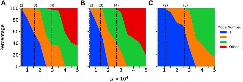
FIGURE 7. Distribution of the most unstable mode in extensional Brownian simulations in instances where the filament crossed the Brownian noise floor threshold for (A) B₁(s), (B) B₂(s), and (C) B₃(s). The dot-dashed lines on each graph, denoted with (2), (3), or (4) represent the calculated onset of instability for the second, third, and fourth modes respectively (see Table 2 for the critical $\bar{\mu }$ values).

To quantitatively compare stability analysis with simulations, we average out our ensemble data by computing the root-mean-squared amplitude across ensembles and extracting a growth rate like above. Like our previous analysis, we filter for amplitude values above the noise floor and on short time scales. Figure 8 shows the growth rate of the most unstable mode from the average ensemble simulation data plotted along with the maximum growth rate from our linear stability analyses. Again, we see that stability predictions and stochastic non-linear simulations are fairly consistent in the mode that is most excited as well as in the magnitude of the growth rate.

FIGURE 8

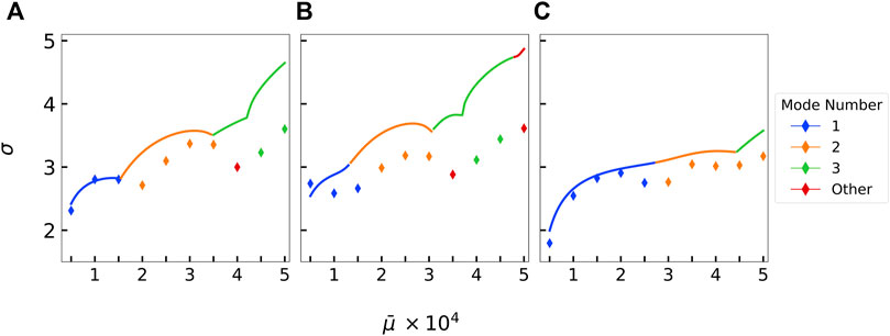
FIGURE 8. Comparison of the predicted growth rates obtained from linear stability analysis against the calculated growth rates from the Brownian extensional simulations at ℓ_p/L =100 along with their corresponding mode number classifications for (A) B₁(s), (B) B₂(s), and (C) B₃(s). The highest growth rates from either stability analysis or simulations are plotted. Lines represent the stability analysis predictions. Diamond points represent the extracted growth rate from the simulations.

4 Conclusion

In summary, we have developed a framework for slender-body theory to incorporate non-uniform bending stiffness of flexible filaments. We use this platform to examine the flow-induced buckling behavior of realistic microfilaments with a non-uniform elastic backbone. As a demonstration of the method and mathematical tools, we model the adsorption or desorption of proteins to result in a locally or asymmetrically weaker or stiffer microfilament. We study the effects of the altered stiffness profiles in simple shear flow, where regions of modified filament backbone give rise to differences in the buckling patterns, tension, elastic energy, and stress tensor components. By comparing the short-time evolution of our Brownian and non-linear simulations to linear stability analyses for each of the κ(s) profiles, we are able to highlight features of enhanced or reduced local filament stiffness.

The model stiffness profiles considered in this work allowed us to arrive at tractable filament shapes and illustrate a consistent set of steps to extract mode shapes from simulations. However, we emphasize that the mathematical machinery developed here is applicable to any modeled or experimentally measured profile of the filament rigidity. We have established the fundamental basis for this direction of analysis of stiff biopolymers such as microtubules with non-uniform protein condensation (Hernández-Vega et al., 2017; Setru et al., 2021). It remains to be seen how this description carries over to more complex flows or to substrate attachments that arise in the experimental tracking of such microtubules (Tan et al., 2019), and how these differences in buckling behavior translate to large-scale filament dispersion (Manikantan and Saintillan, 2013) or cross-streamline migration (Xue et al., 2022). Our model can be readily extended to temporal variations in filament stiffness as well, setting the stage for future work on finite-time kinetics of protein adsorption/desorption and the elastohydrodynamics associated with such a process. We anticipate that the tools and insights gathered in the current work will support these future research directions.

Data availability statement

The raw data supporting the conclusion of this article will be made available by the authors, without undue reservation.

Author contributions

TN and HM designed research, performed analysis and simulations, and wrote the manuscript.

Acknowledgments

We acknowledge financial support from a GAANN fellowship (TN) and a Hellman Foundation fellowship (HM).

Conflict of interest

The authors declare that the research was conducted in the absence of any commercial or financial relationships that could be construed as a potential conflict of interest.

Publisher’s note

All claims expressed in this article are solely those of the authors and do not necessarily represent those of their affiliated organizations, or those of the publisher, the editors and the reviewers. Any product that may be evaluated in this article, or claim that may be made by its manufacturer, is not guaranteed or endorsed by the publisher.

References

Baczynski, K., Lipowsky, R., and Kierfeld, J. (2008). Stretching of buckled filaments by thermal fluctuations. Phys. Rev. E - Stat. Nonlinear, Soft Matter Phys. 76, 061914–061919. doi:10.1103/physreve.76.061914

PubMed Abstract | CrossRef Full Text | Google Scholar

Batchelor, G. K. (1970). Slender-body theory for particles of arbitrary cross-section in Stokes flow. J. Fluid Mech. 44, 419–440. doi:10.1017/s002211207000191x

CrossRef Full Text | Google Scholar

Batchelor, G. K. (1970). The stress system in a suspension of force-free particles. J. Fluid Mech. 41, 545–570. doi:10.1017/s0022112070000745

CrossRef Full Text | Google Scholar

Becker, L. E., and Shelley, M. J. (2001). Instability of elastic filaments in shear flow yields first-normal-stress differences. Phys. Rev. Lett. 87, 198301–198304. doi:10.1103/physrevlett.87.198301

PubMed Abstract | CrossRef Full Text | Google Scholar

Chakrabarti, B., Liu, Y., LaGrone, J., Cortez, R., Fauci, L., du Roure, O., et al. (2020). Flexible filaments buckle into helicoidal shapes in strong compressional flows. Nat. Phys. 16, 6891910689–6891910694. doi:10.1038/s41567-020-0843-7

CrossRef Full Text | Google Scholar

Chakrabarti, B., Gaillard, C., and Saintillan, D. (2020). Trapping, gliding, vaulting: Transport of semiflexible polymers in periodic post arrays. Soft Matter 16, 5534–5544. doi:10.1039/d0sm00390e

PubMed Abstract | CrossRef Full Text | Google Scholar

Chakrabarti, B., Liu, Y., Du Roure, O., Lindner, A., and Saintillan, D. (2021). Signatures of elastoviscous buckling in the dilute rheology of stiff polymers. J. Fluid Mech. 919. arXiv:2102.11407. doi:10.1017/jfm.2021.383

CrossRef Full Text | Google Scholar

Chelakkot, R., Winkler, R. G., and Gompper, G. (2010). Migration of semiflexible polymers in microcapillary flow. Europhys. Lett. 91, 14001. doi:10.1209/0295-5075/91/14001

CrossRef Full Text | Google Scholar

Chelakkot, R., Winkler, R. G., and Gompper, G. (2012). Flow-induced helical coiling of semiflexible polymers in structured microchannels. Phys. Rev. Lett. 109, 178101–178105. doi:10.1103/physrevlett.109.178101

PubMed Abstract | CrossRef Full Text | Google Scholar

De La Cruz, E. M., Martiel, J. L., and Blanchoin, L. (2015). Mechanical heterogeneity favors fragmentation of strained actin filaments. Biophysical J. 108, 2270–2281. doi:10.1016/j.bpj.2015.03.058

CrossRef Full Text | Google Scholar

Girard, M., de la Cruz, M. O., Marko, J. F., and Erbaş, A. (2020). Heterochromatin flexibility contributes to chromosome segregation in the cell nucleus. bioRxiv [Preprint]. Available at: https://www.biorxiv.org/content/10.1101/2020.12.01.403832v1.

Google Scholar

Gittes, F., Mickey, B., Nettleton, J., and Howard, J. (1993). Flexural rigidity of microtubules and actin filaments measured from thermal fluctuations in shape. J. Cell Biol. 120, 923–934. doi:10.1083/jcb.120.4.923

PubMed Abstract | CrossRef Full Text | Google Scholar

Guglielmini, L., Kushwaha, A., Shaqfeh, E. S., and Stone, H. A. (2012). Buckling transitions of an elastic filament in a viscous stagnation point flow. Phys. Fluids 24, 123601. doi:10.1063/1.4771606

CrossRef Full Text | Google Scholar

Harasim, M., Wunderlich, B., Peleg, O., Kröger, M., and Bausch, A. R. (2013). Direct observation of the dynamics of semiflexible polymers in shear flow. Phys. Rev. Lett. 110, 108302–108305. doi:10.1103/physrevlett.110.108302

PubMed Abstract | CrossRef Full Text | Google Scholar

Hernández-Vega, A., Braun, M., Scharrel, L., Jahnel, M., Wegmann, S., Hyman, B. T., et al. (2017). Local nucleation of microtubule bundles through tubulin concentration into a condensed tau phase. Cell Rep. 20, 2304–2312. doi:10.1016/j.celrep.2017.08.042

PubMed Abstract | CrossRef Full Text | Google Scholar

Johnson, R. E. (1980). An improved slender-body theory for Stokes flow. J. Fluid Mech. 99, 411–431. doi:10.1017/s0022112080000687

CrossRef Full Text | Google Scholar

Kantsler, V., and Goldstein, R. E. (2012). Fluctuations, dynamics, and the stretch-coil transition of single actin filaments in extensional flows. Phys. Rev. Lett. 108, 038103–038105. doi:10.1103/physrevlett.108.038103

PubMed Abstract | CrossRef Full Text | Google Scholar

Keller, J. B., and Rubinow, S. I. (1976). Slender-body theory for slow viscous flow. J. Fluid Mech. 75, 705–714. doi:10.1017/s0022112076000475

CrossRef Full Text | Google Scholar

Landau, L., and Lifshitz, E. M. (1986). Course of theoretical Physics. 3rd ed. Oxford: Pergamon Press.

Google Scholar

Li, L., Manikantan, H., Saintillan, D., and Spagnolie, S. E. (2013). The sedimentation of flexible filaments. J. Fluid Mech. 735, 7051306–7364692. doi:10.1017/jfm.2013.512

CrossRef Full Text | Google Scholar

Liu, Y., Chakrabarti, B., Saintillan, D., Lindner, A., and Du Roure, O. (2018). Morphological transitions of elastic filaments in shear flow. Proc. Natl. Acad. Sci. U. S. A. 115, 9438–9443. arXiv:1803.10979. doi:10.1073/pnas.1805399115

PubMed Abstract | CrossRef Full Text | Google Scholar

Lorenzo, A. M., Koslover, E. F., and De La Cruz, E. M. (2020). Thermal fracture kinetics of heterogeneous semiflexible polymers. Soft Matter 16, 2017–2024. arXiv:1905.03327. doi:10.1039/c9sm01637f

PubMed Abstract | CrossRef Full Text | Google Scholar

Manikantan, H., and Saintillan, D. (2013). Subdiffusive transport of fluctuating elastic filaments in cellular flows. Phys. Fluids 25, 073603–073614. doi:10.1063/1.4812794

CrossRef Full Text | Google Scholar

Manikantan, H., and Saintillan, D. (2015). Buckling transition of a semiflexible filament in extensional flow. Phys. Rev. E - Stat. Nonlinear, Soft Matter Phys. 92, 041002–041004. doi:10.1103/physreve.92.041002

PubMed Abstract | CrossRef Full Text | Google Scholar

Manikantan, H. (2015). “Bending, buckling, tumbling, trapping: Viscous dynamics of elastic filaments,” PhD dissertation (San Diego, Engineering Sciences: University of California).

Google Scholar

Munk, T., Hallatschek, O., Wiggins, C. H., and Frey, E. (2006). Dynamics of semiflexible polymers in a flow field. Phys. Rev. E - Stat. Nonlinear, Soft Matter Phys. 74, 041911–11. doi:10.1103/physreve.74.041911

PubMed Abstract | CrossRef Full Text | Google Scholar

Quennouz, N., Shelley, M., Du Roure, O., and Lindner, A. (2015). Transport and buckling dynamics of an elastic fibre in a viscous cellular flow. J. Fluid Mech. 769, 387–402. doi:10.1017/jfm.2015.115

CrossRef Full Text | Google Scholar

Setru, S. U., Gouveia, B., Alfaro-aco, R., Shaevitz, J. W., Stone, H. A., and Petry, S. (2021). A hydrodynamic instability drives protein droplet formation on microtubules to nucleate branches. Nat. Phys. 17, 493–498. doi:10.1038/s41567-020-01141-8

PubMed Abstract | CrossRef Full Text | Google Scholar

Suzuki, K., Miyazaki, M., Takagi, J., Itabashi, T., and Ishiwata, S. (2017). Spatial confinement of active microtubule networks induces large-scale rotational cytoplasmic flow. Proc. Natl. Acad. Sci. U. S. A. 114, 2922–2927. doi:10.1073/pnas.1616001114

PubMed Abstract | CrossRef Full Text | Google Scholar

Tan, R., Lam, A. J., Tan, T., Han, J., Nowakowski, D. W., Vershinin, M., et al. (2019). Microtubules gate tau condensation to spatially regulate microtubule functions. Nat. Cell Biol. 21, 1078–1085. doi:10.1038/s41556-019-0375-5

PubMed Abstract | CrossRef Full Text | Google Scholar

Tornberg, A. K., and Shelley, M. J. (2004). Simulating the dynamics and interactions of flexible fibers in Stokes flows. J. Comput. Phys. 196, 8–40. doi:10.1016/j.jcp.2003.10.017

CrossRef Full Text | Google Scholar

Verchot-Lubicz, J., and Goldstein, R. E. (2010). Cytoplasmic streaming enables the distribution of molecules and vesicles in large plant cells. Protoplasma 240, 99–107. doi:10.1007/s00709-009-0088-x

PubMed Abstract | CrossRef Full Text | Google Scholar

Wandersman, E., Quennouz, N., Fermigier, M., Lindner, A., and Du Roure, O. (2010). Buckled in translation. Soft Matter 6, 5715–5719. doi:10.1039/c0sm00132e

CrossRef Full Text | Google Scholar

Wiggins, C. H., Riveline, D., Ott, A., and Goldstein, R. E. (1998). Trapping and wiggling: Elastohydrodynamics of driven microfilaments. Biophysical J. 74, 1043–1060. doi:10.1016/s0006-3495(98)74029-9

PubMed Abstract | CrossRef Full Text | Google Scholar

Woodhouse, F. G., and Goldstein, R. E. (2013). Cytoplasmic streaming in plant cells emerges naturally by microfilament self-organization. Proc. Natl. Acad. Sci. U. S. A. 110, 14132–14137. doi:10.1073/pnas.1302736110

PubMed Abstract | CrossRef Full Text | Google Scholar

Xue, N., Nunes, J. K., and Stone, H. A. (2022). Shear-induced migration of confined flexible fibers. Soft Matter 18, 514–525. doi:10.1039/d1sm01256h

PubMed Abstract | CrossRef Full Text | Google Scholar

Young, Y. N., and Shelley, M. J. (2007). Stretch-coil transition and transport of fibers in cellular flows. Phys. Rev. Lett. 99, 058303–058306. doi:10.1103/physrevlett.99.058303

PubMed Abstract | CrossRef Full Text | Google Scholar