Estimation of the Optimal Spherical Harmonics Order for the Interpolation of Head-Related Transfer Functions Sampled on Sparse Irregular Grids

1 Introduction

Head-Related Transfer Functions (HRTFs) are essential for the binaural reproduction of virtual acoustic environments (Vorländer, 2008). In contrast to commonly used generic HRTFs, individual HRTFs improve the perceived quality of binaural reproduction in terms of front/back localization and elevation perception (Wenzel et al., 1993; Møller et al., 1996). However, conventional measurements of individual HRTF sets are costly in time and effort. Even though recent achievements reduced the required measurement time (Majdak et al., 2007; Enzner et al., 2013; Richter, 2019), most measurement systems still rely on rather complex immobile setups, such as (semi-)circular loudspeaker arcs, where a full-spherical coverage of measurement directions needs a continuous rotation of the subject or the installation. Besides measurements, there are also alternative methods to obtain individual HRTFs (Guezenoc and Seguier, 2018), such as numerical simulation from 3D models (Pollack and Majdak, 2021) or individualization of generic HRTFs (Bomhardt, 2017). Even though those methods mostly have some shortcomings compared to measurements, they primarily target a consumer audience, where their simplicity justifies their relevance.

To simplify individual HRTF measurements and prevent the need for costly measurement setups, some recently introduced systems utilize free body movements (FBM; such systems are in the following called FBM systems) of the subject to cover the different sound incidence angles. Characteristic to these FBM systems are the low equipment requirements, that is, a single stationary loudspeaker, a pair of in-ear microphones, and a system to track the head orientation with respect to the stationary loudspeaker. The system presented in He et al. (2018) uses adaptive filtering to acquire HRTFs from a continuous excitation signal, while the head orientation is tracked with an inertial measurement unit (IMU). A similar system was also implemented by Li and Peissig (2017). HRTF measurements using adaptive filtering, introduced by Enzner (2008), yield spatially continuous HRTFs, given a sufficiently slow and known rotation speed, and do not require any successive interpolation. However, adaptive filtering is less robust against environmental noise than commonly used exponential sine sweep (ESS) measurements (Fallahi et al., 2015), making it rather inappropriate for use in normal rooms. Reijniers et al. (2020) presented a system that uses an optical tracking system for the head movements and short ESS for measurements at discrete sampling points. Similarly, our recently proposed system (Bau et al., 2021) is based on ESS measurements but uses a commercially available virtual reality system for tracking. With the latter two systems, measurements can be performed even in reverberant conditions, meaning that an anechoic chamber is not mandatory. In general, FBM systems have some properties that can have a negative effect on the measurement. Major sources of errors are inaccuracies of the tracking devices, reflections of the torso at various orientations, and in case the measurements are carried out in reflective environments the influence of the room acoustics. However, recent studies showed that these effects can be successfully mitigated or neglected (Pörschmann and Arend, 2019a; Pörschmann and Arend, 2019b; Reijniers et al., 2020; Bau and Pörschmann, 2022). As such, FBM systems, especially due to their simple design, offer a promising approach for obtaining high-quality individual HRTFs by facilities that are not specialized in acoustic measurements.

However, having no fixed measurement installation implies that the measurement directions of HRTFs typically do not correspond to predefined sampling grids. Instead, FBM systems usually provide HRTF measurements on irregular grids, meaning for directions irregularly distributed along a virtual sphere. Moreover, depending on the measurement effort, typically only a small number of directions are captured. To obtain meaningful HRTF sets, spatial interpolation of such irregularly and sparsely sampled measurement data is necessary. In the past, various approaches for HRTF interpolation have been proposed. Already in 1993, Wenzel and Foster (1993) stated that localization accuracy was largely unaffected by discontinuous nearest-neighbor interpolation, even for large interpolation intervals. Chen et al. (1995) used a weighted combination of Eigen transfer functions obtained by feature extraction to synthesize interpolated HRTFs. Djelani et al. (2000) aligned the HRTFs in the time-domain prior to interpolation to mitigate interpolation errors. Separate interpolation of magnitude and unwrapped phase delivered similarly good results (Hartung et al., 1999). The interpolation weights can be derived in different ways, including natural neighbor (Sibson, 1981; Pörschmann et al., 2020), spline-based interpolation (Hartung et al., 1999), or barycentric weights (Shirley and Marschner, 2009, Chap. 2) as, for example, used by Gamper (2013).

Describing and interpolating HRTFs in the spherical harmonics (SH) domain is an efficient and recently quite popular approach. (Evans et al., 1998; Richter, 2019; Arend et al., 2021). However, the highest representable frequency is limited by the SH order N, following the relation N ∼ kr (Rafaely and Avni, 2010). Here, k denotes the wavenumber and r the radius of the smallest sphere surrounding the head. Thus, for a correct interpolation up to 20 kHz with an average head radius of r = 0.0875 m, an SH order of N_max ≈ 32 is required, resulting in a minimum of ${(N_{\max }+1)}^2=1089$ measurement directions. Sparsely measured HRTF sets with N_sparse < N_max cannot meet this requirement and their SH representation suffers from so-called sparsity errors (see Section 2.2). Various recent publications investigated SH interpolation of sparse HRTF sets and the associated sparsity errors (Ben-Hur et al., 2019; Arend et al., 2021). These studies only considered sparse HRTF sets sampled on regular (explicitly defined) grids, for which the SH order is usually known (Zotter, 2009b) (Rafaely, 2015, Chap. 3). However, to the best of our knowledge, the effects on SH interpolation when using irregular grids (e.g., from FBM systems) have not been investigated systematically yet. Furthermore, a general rule for choosing an appropriate SH order for interpolation of irregular sampled HRTFs has also not been given so far.

This study investigates SH interpolation of selected irregular sampling grids obtained from HRTF measurements with our FBM system (Bau et al., 2021) to find the optimal SH order for interpolation. The sparse sets are spatially interpolated to a dense reference grid using state-of-the-art pre- and postprocessing methods in combination with SH interpolation. The study analyzes how the variation of the SH order affects and ideally improves the interpolation results and how applying the commonly used Tikhonov regularization (see Section 2.4) affects the results. We show that the optimal SH order, that is, the one resulting in the lowest interpolation errors, depends strongly on the irregular sampling grid and the regularization but is almost independent of the HRTF set. Based on these results, we propose a simple method for estimating the optimal SH order for HRTFs measured on irregular grids, such as those obtained with FBM systems: The irregular grid of the FBM measurement is used to derive a substitute HRTF set from a dense reference HRTF set. Then, the optimal SH order is derived from interpolation and subsequent error evaluation of the substitute set. To evaluate the proposed method, we compare the interpolation error of irregular grids with that of regular grids, both interpolated with the same SH order. We show that when the optimal SH order (of the irregular grid) is determined by the proposed method, irregular grids lead to very similar interpolation results as the well-studied regular grids.

2 Spherical Harmonics Interpolation of HRTF Data

2.1 Spherical Harmonics Interpolation and Least-Squares Solution

Spherical harmonics provide an efficient way to represent HRTF data H^L/R for the left and right ear sampled at a finite number of measurement directions Ω (Duraiswami et al., 2004) (indices for the left and right ear are omitted in the following whenever the processing is identical for both ears). The direction Ω = (ϕ, θ) is defined by the azimuth ϕ = [0°, 360°] and the elevation θ = [ − 90°, 90°], whereby ϕ is measured counterclockwise in the xy-plane, starting at positive x, and θ is 90° at positive z. From a set of (order limited) SH coefficients h_nm, a set of HRTFs H can be obtained for any direction Ω_q with the discrete inverse spherical Fourier transform (ISFT) by

$H=Y{h}_{nm}(1)$

where Y is the Q × (N + 1)² SH matrix of SH basis functions, with

$Y=\left[\begin{array}{ccccc}\hfill Y_0^0\left({\mathrm{\Omega }}_1\right)\hfill & \hfill Y_1^{-1}\left({\mathrm{\Omega }}_1\right)\hfill & \hfill Y_1^0\left({\mathrm{\Omega }}_1\right)\hfill & \hfill \cdots \hfill & \hfill Y_N^N\left({\mathrm{\Omega }}_1\right)\hfill \\ \hfill Y_0^0\left({\mathrm{\Omega }}_2\right)\hfill & \hfill Y_1^{-1}\left({\mathrm{\Omega }}_2\right)\hfill & \hfill Y_1^0\left({\mathrm{\Omega }}_2\right)\hfill & \hfill \cdots \hfill & \hfill Y_N^N\left({\mathrm{\Omega }}_2\right)\hfill \\ \hfill ⋮\hfill & \hfill ⋮\hfill & \hfill ⋮\hfill & \hfill \ddots \hfill & \hfill ⋮\hfill \\ \hfill Y_0^0\left({\mathrm{\Omega }}_Q\right)\hfill & \hfill Y_1^{-1}\left({\mathrm{\Omega }}_Q\right)\hfill & \hfill Y_1\left({\mathrm{\Omega }}_Q\right)\hfill & \hfill \cdots \hfill & \hfill Y_N^N\left({\mathrm{\Omega }}_Q\right)\hfill \end{array}\right](2)$

Each row can be interpreted as a sampling direction Ω_Q, and the columns represent the SH coefficients up to order N.

The spherical Fourier transform (SFT), or also SH transform, to obtain h_nm from a set of HRTFs sampled at a sufficient number of measurement directions Q ≥ (N + 1)² corresponds to solving the overdetermined linear system in Eq. 1 in a least-squares sense to yield

$h_{nm}=Y^{†}H,(3)$

where $Y^{†}={(Y^{H}Y)}^{-1}{Y}^H$ is the pseudo-inverse of Y. By substituting Eq. 3 in Eq. 1, the SH interpolation of the origin Q-direction set H to a target T-point set $\widehat{H}$ can be described as:

$\widehat{H}=Y_t{Y}_q^{†}H(4)$

where Y_t and Y_q are the SH matrices of size T × (N + 1)² and Q × (N + 1)², associated with the sampling directions Ω_t and Ω_q, respectively.

2.2 Sparsity Errors

A sparsely sampled HRTF set can usually only be transformed to the SH domain with a low SH order N_sparse < N_max. This leads to order truncation effects, resulting in lower spatial resolution and high-frequency attenuation (Bernschütz et al., 2014). Furthermore, an insufficient number of measurement directions Q causes spatial aliasing, resulting in spatial ambiguities and increased energy in higher frequencies above the so-called spatial aliasing frequency (Rafaely, 2005). Together, truncation and aliasing errors form the sparsity error, also frequently called undersampling error. A detailed insight into the respective contribution to the overall sparsity error is given in Ben-Hur et al. (2019).

The perceptual impact of sparsity errors on the spectral and temporal structure of the HRTF was subject to several recent studies with the aim to estimate a lower bound for the SH order at which an HRTF can be successfully represented. Romigh et al. (2015) found in their technical analysis a maximum error of 1 dB between 300 Hz and 14 kHz at an SH order of N = 14, and in an empirical study a largely preserved localization accuracy at N = 4. They concluded that technical evaluation results might be gross overestimates of a minimum SH order compared to perceived error. In a perceptual study, Pike (2019) evaluated the perceivable error of SH interpolation, where interpolation was also performed on time-aligned HRTFs. At N = 5 and with time-alignment, only low perceptual impact was found for frontal directions, while clear differences remained for lateral source positions. A listening experiment by Arend et al. (2021) to evaluate SH interpolation of time-aligned HRTFs using one selected approach yielded similar results, revealing a minimum required SH order for perceptually transparent SH interpolation of N = 7 and N = 10 for frontal speech and noise sources, respectively. For lateral directions, the minimum required SH orders were substantially higher, with N ≈ 17 and N ≈ 22 for speech and noise sources, respectively. Notably, the different time-alignment methods technically evaluated in this study performed similarly well, with notable differences only at very low SH orders and contralateral HRTFs. Based on this, it was suggested that the methods can be used equivalently.

2.3 Condition Number and Numerical Stability

The condition number κ is defined by the ratio of the largest to smallest singular value in the singular value decomposition of a matrix (Lichtblau and Weisstein, 2022). If κ is too large, a linear system, such as Eq. 1 or Eq. 3, is considered ill-conditioned and will become unstable, resulting in an unpredictable output for a given input. In general, a low condition number indicates a system with high rank where the rows are mostly linearly independent. Since the rows of the SH matrix Y represent the sampling points, κ can be used as a measure for grid efficiency (Zotter, 2009b). Furthermore, for a sampling grid Ω, where no maximum SH order is given explicitly by its configuration, the conditioning of Y can estimate if a proposed SH order can be used for a stable least-squares solution. For a deeper analysis of the condition number for the SH matrix Y, please refer to Reddy and Hegde (2017).

The condition number is often used for characterising the stability of the least-squares solution (Zotter, 2009a; Zotkin et al., 2009; Pike, 2019). Ben-Hur et al. (2019) considered sampling grids with a condition number below 3.5 as stable. However, to the best of our knowledge, there is not yet a general rule for using κ to decide whether or not a sampling grid can be considered stable for a particular SH order. Problematic in this sense is the indistinct relationship between κ and the resulting error of the least-squares SFT. In terms of numerical computation, the condition number describes the sensitivity of a least-squares solution to perturbations of the input. Depending on the underlying problem and the demands on the error tolerance of the solution, κ can vary significantly and the results can still be considered as acceptable (Demmel, 1997).

2.4 Regularization

Numerous ways to regularize ill-conditioned problems exist (Hansen, 1994). The regularization proposed by Tikhonov et al. (1995) is commonly used in the field of virtual acoustics for stabilizing the SH transform for incomplete sampling grids, such as when the lower cap of the sampling sphere is missing due to the design of the measurement system (Zhang et al., 2010; Ahrens et al., 2012; Pollow et al., 2012; Richter and Fels, 2019). By applying regularization to the inversion of Y, Eq. 3 becomes

$h_{nm}={\left(Y^{T}Y+ϵD\right)}^{-1}{Y}^{T}H(5)$

where ϵ controls the regularization amount and D is a diagonal damping matrix as proposed by Duraiswami et al. (2004):

$D=\left(1+n\left(n+1\right)\right)I,(6)$

where n denotes the degree of the corresponding basis function $Y_n^m$ and I is the identity matrix.

Although routines exist to determine a suitable value for ϵ, such as L-curve or Picard condition (Hansen, 1994), in practice ϵ is commonly set by hand for a specific problem. Duraiswami et al. (2004) set ϵ to 10⁻⁶, Zhang et al. (2010) used a value of 10⁻⁵. Pollow et al. (2012) found that a lower value of 10⁻⁸ provides better interpolation results at high frequencies and Richter and Fels (2019) used regularization with ϵ = 10⁻⁸ to stabilize a grid with 4,608 points and a missing bottom cap. Furthermore, Tikhonov regularization can also be used for complete grids to mitigate the influence of measurement noise (Pike, 2019, Chap. A.7).

3 Interpolation Analysis

We investigated the interpolation error of HRTF data sampled on six irregular sampling grids as shown in Figure 1. The grids are representative example results of our FBM system (Bau et al., 2021), where subjects followed different strategies to obtain spherical sampling. The first two grids Irregular 1 and Irregular 2, each with 40 sampling points, can be considered as very sparse and represent a minimal configuration. Irregular 3 and Irregular 4 with 68 and 73 points represent a compromise between measurement time and accuracy. The grids Irregular 5 and Irregular 6 with 118 and 117 points can be considered as fairly well sampled, but depending on the measurement system, the acquisition can be quite time-consuming (the time required for those sets with our FBM system was about 20 min). For comparison, two common regular sampling grids were added, a Gaussian and a Lebedev sampling grid with 128 and 86 points, respectively.

FIGURE 1

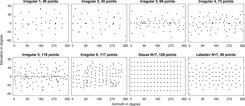
FIGURE 1. Examined six irregular test sampling grids and two regular grids for comparison.

3.1 Interpolation Procedure

To be able to examine the interpolation error isolated from other potential measurement influences, we avoided to use the actual HRTF data from the irregular measurements. Instead, we used numerically simulated individual HRTFs of a randomly chosen subject (no. 10) from the HUTUBS database (Brinkmann et al., 2019) as a reference. The HRTFs of the reference set are stored on a 1730-point Lebedev sampling grid, allowing for SH representation up to order N = 35 and thus perceptually correct representation of the entire frequency-range of an HRTF (see Section 1). The reference HRTF set was spatially resampled to the different irregular sampling grids to obtain the artificial irregular HRTF sets for the interpolation analysis.

We interpolated the irregular HRTF sets to a dense 1202-point Lebedev grid in the SH domain according to Eq. 4. Prior to SH interpolation, the HRTF sets were time-aligned, which lowers the spatial complexity and thus reduces the required SH order and consequently the interpolation errors (Arend et al., 2021). A relative time-alignment was performed by division with matching rigid sphere transfer functions using the SUpDEq method (Pörschmann et al., 2019a; Arend et al., 2021). After the interpolation, the phase and magnitude components were recovered by spectral multiplication with corresponding rigid sphere transfer functions for the directions of the dense grid. In informal evaluations, we compared various time-alignment procedures when interpolating irregular HRTF sets, similar to what Arend et al. (2021) did for regular HRTF measurements. Supplementary Figures S1–S4 show an according comparison of different preprocessing methods. As the results showed great similarity, we chose SUpDEq as the default preprocessing method.

The interpolation was repeated for each grid with different SH order, starting from N = 1 up to N_max for the respective grid following $Q\ge {(N_{\max }+1)}^2$. For each grid and SH order, we additionally performed SH interpolations using a regularized inversion of Y according to Section 2.4 with ϵ = {10⁻⁴, 10⁻³, 10⁻²}. The lowest regularization parameter value represents a conservative value, based on previous studies as mentioned in Section 2.4. The highest value was chosen empirically during our evaluation as it provided the best results for the sparse irregular sampling grids presented here.

In order to get a useful error metric of the interpolation performance, we compared every interpolated HRTF set to the reference set and evaluated the magnitude error and ITD differences. These metrics were recently used to analyze interpolation errors by Arend et al. (2021) and showed good accordance to the results of the perceptual evaluation.

The magnitude error ΔG (f_c, Ω) was calculated as the absolute difference in dB between HRTF magnitudes in 41 auditory filter bands (Slaney, 1998) with center frequency f_c for every sampling point Ω, in the frequency range from 50 Hz to 20 kHz. The magnitude error for left and right ear of the HRTF are largely equivalent, so for simplicity only the left ear magnitude error is considered in the following. For a more comprehensible error, the error was averaged over the auditory filter bands to yield the spatial error distribution ΔG(Ω) and over the sampling points to yield the frequency error distribution ΔG (f_c). By averaging over both frequency and sampling points, a scalar magnitude error ΔG was obtained.

The ITDs were calculated as the difference from the time-of-arrivals (TOAs) for the left and right ear. The TOAs were determined by onset detection from the low-pass filtered (eighth order Butterworth, f_c = 3 kHz) and 10 times upsampled HRIRs, as proposed by Andreopoulou and Katz (2017). An onset threshold of −10 dB in relation to the maximum values was used for the TOA estimation, as proposed by Arend et al. (2021). The ITD difference was then calculated for every sampling point as the absolute difference between the ITD of the reference set and the ITD of the interpolated set.

3.2 Interpolation Error at Different Spherical Harmonics Orders

In this section, we evaluate the overall magnitude error ΔG from interpolation with different SH orders according to Section 3.1 to estimate the optimal SH order for each grid as a trade-off between sparsity error and the error of the least-squares solution. Figure 2A shows how different SH orders affect the interpolation results. As expected, the sparsity error decreases with increasing order. At a certain order, without regularization, the error starts to increase again. At this point, the least-squares solution to the matrix Y becomes more and more ill-conditioned and numerical errors occur.

FIGURE 2

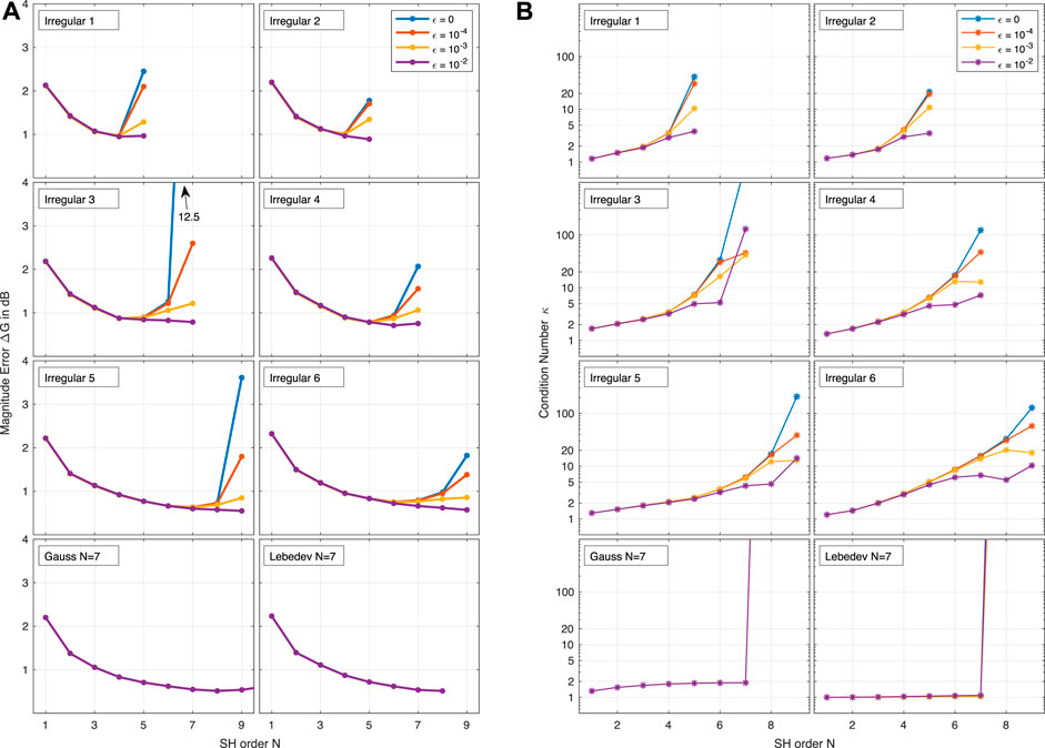
FIGURE 2. (A) Left-ear magnitude error ΔG with respect to SH order for six examined irregular grids and two regular grids with different regularization values ϵ. HRTF: Subject no. 10 from HUTUBS database. (B) Corresponding condition number κ of Y^† with respect to SH order and regularization value ϵ.

In the topmost row of Figure 3, this decrease and increase of the error can be observed for the spatial error distribution ΔG(Ω) on the example of grid Irregular 6 and selected SH orders. Further plots for other examined grids and SH orders are provided in the Supplementary Figures S5–S20. Both Figure 2A and Figure 3 show that regularization can limit the error towards higher orders. Without regularization, the error in certain spatial regions increases dramatically towards higher orders. A comparison with the corresponding sampling grid in Figure 1 shows that these regions are related to the sampling grid. With regularization, however, the SH transform can be stabilized and the error decreases, even for the highest possible SH order N_max, as can be seen in Figure 2A. Apart from this, regularization does not affect the magnitude error for lower SH orders. For Supplementary Figures S5–S20 in the supplementary material, we also included interpolations using higher regularization values to show that regularization values above 10⁻² result in an increased error for both magnitude and ITD. Notably, Tikhonov regularization has no impact on the regular sampling grids.

FIGURE 3

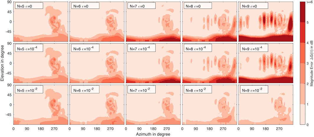
FIGURE 3. Left-ear magnitude error ΔG(Ω) for grid Irregular 6 at selected SH orders and regularization values ϵ. HRTF: Subject no. 10 from HUTUBS database.

Figure 4 shows the horizontal plane ITD difference for grid Irregular 6 for selected SH orders and regularization values ϵ by means of differences to the reference ITD. The gray area denotes the broadband just noticeable difference (JND) as a function of the reference ITD (Mossop and Culling, 1998). To approximate the JND across all azimuthal positions, it was linearly interpolated between 20 μs at ITD_ref = 0 and 100 μs at ITD_ref = 700 μs Overall, the ITD differences remain well below the JND for all examined conditions. This is in accordance with the findings of Arend et al. (2021), where the time-aligned interpolation of HRTFs is unproblematic in regards to ITD, even at very low SH orders. Only for N = 9 without regularization, the ITD difference increases again significantly and almost exceeds the JND.

FIGURE 4

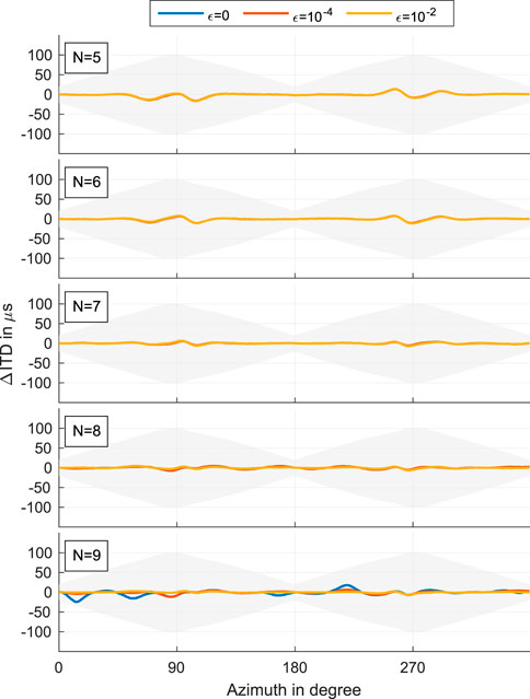
FIGURE 4. Difference in horizontal plane ITD relative to the dense reference for grid Irregular 6 at selected SH orders and regularization values ϵ. The shaded area denotes the JND as a function of the reference ITD. HRTF: Subject no. 10 from HUTUBS database.

An analytical prediction of the point of instability, meaning where the numerical errors of the least-squares solution become overly large, would be of great benefit. In a first approach, we evaluated the condition number κ of Y^† to establish a relationship between the error ΔG and κ. Figure 2B shows κ with respect to the SH order N for all examined grids and different regularization values ϵ. Even though a general relation between error and condition number is visible, a clear determination of a threshold value for κ that ensures least-squares stability is not directly possible. In general, the results indicate that the interpolation is stable for κ < 10. However, for some grids, such as Irregular 6, the lowest error without regulariazion is at N = 7 with κ ≈ 18. Because of this relatively unpredictable behavior of κ, we assume that estimating the optimal SH order based on the condition number is inappropriate.

3.3 Method for Estimating the Optimal Spherical Harmonics Order

Figure 2A shows that the optimal SH order for each artificial HRTF set can be derived from the lowest associated magnitude error ΔG. However, for sparse measurements made in practice with an FBM system, a dense reference is usually unavailable, and it is impossible to calculate the required error from the measurement data. Yet, suppose the interpolation errors of different artificial reference HRTF sets (i.e., HRTF sets obtained by resampling different dense reference sets to the individually measured sparse irregular grid) show a similar pattern as a function of the SH order. In that case, it is most likely that the optimal SH order thus obtained can be applied to real individual HRTF measurements on the same irregular grid. From this consideration, our approach follows to determine the optimal (grid-dependent) SH order for the individual measurements as the minimum magnitude error ΔG obtained with a dense reference HRTF set.

To show that the interpolation error curve has a consistent shape across different HRTF sets, we repeated the calculation of the magnitude error (see Section 3.1) for the individual HRTFs of all 96 subjects of the HUTUBS database and for a mean HRTF set derived from all 96 subjects by separately averaging magnitude in dB and unwrapped phase. Additionally, for cross-database evaluation, we used generic HRTF sets of a KEMAR head-and-torso simulator (Braren and Fels, 2020), the FABIAN head-and-torso simulator (Brinkmann et al., 2017), a Neumann KU100 dummy head (Bernschütz, 2013), and a Head Acoustics HMS II.3 (Pörschmann et al., 2019b).

Figure 5A shows the resulting magnitude errors for the averaged HUTUBS set (black line) and the 96 individual sets (gray lines) for three examined irregular test grids and different regularization values ϵ. Notably, the general shape of all error curves is similar, and the error curve of the mean HRTF set indeed resembles an average of the individual error curves. This similarity suggests that the error curve of ΔG depends on the sampling grid, but barely on the underlying HRTF set. Hence, it can be used to characterize the sampling grid of an unknown HRTF set. Indeed, the resulting SH order estimations in Figure 5B have very little variance (± 1 N). The mean HRTF, denoted by the red dot, shows great accordance to the individual results. Only the grids Irregular 3 and Irregular 5 with high Tikhonov regularization show slighlty more variance, but only for a very small number of estimates.

FIGURE 5

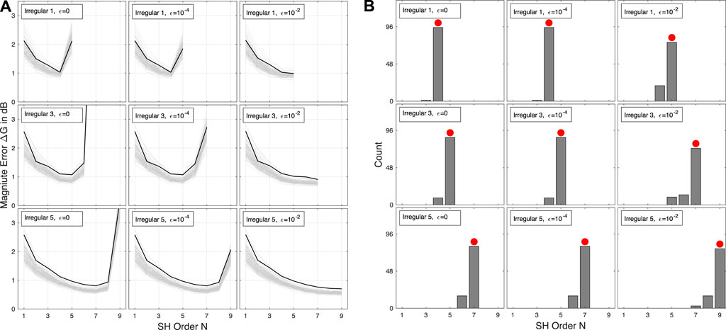
FIGURE 5. (A) Left-ear magnitude error ΔG with respect to SH order for 96 individual HUTUBS HRTF sets (gray lines) and for the averaged HUTUBS HRTF set (black line) for three examined irregular grids and different regularization values ϵ. (B) Distribution of estimated optimal SH orders from the 96 individual HUTUBS HRTF sets (count as Gy bars) and the averaged HUTUBS HRTF set (red dot).

Figure 6 shows the results of the cross-database evaluation. As with the previous analysis, the shape of the error curves, here for all generic HRTF sets examined, is very similar. Only a general offset in the error between HRTF sets can be observed. The offset is a result of the varying spatial complexity of the HRTF datasets, which will have a direct impact on the interpolation error. The KU100 and (simulated) HUTUBS datasets have a lower spatial complexity due to the lack of a torso, whereby the rest of the analyzed datasets include torso reflections. However, as the minimum error for all sets is at the same SH order, there is no impact on the proposed method for determining the optimal SH order. Thus, the estimated optimal SH orders are consistent across the HRTF sets, as summarized in Table 1.

FIGURE 6

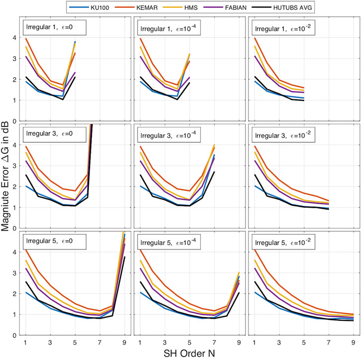
FIGURE 6. Left-ear magnitude error ΔG with respect to SH order for different generic HRTF sets and the averaged HUTUBS HRTF set for three examined irregular grids and different regularization values ϵ.

TABLE 1

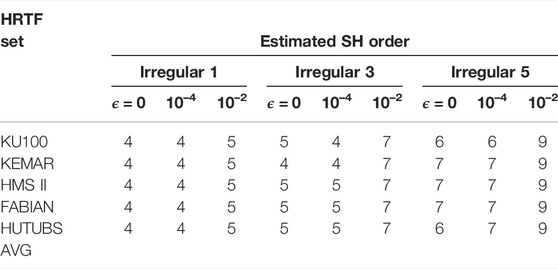
TABLE 1. Estimated optimal SH order for different generic HRTF sets and the averaged HUTUBS HRTF set for three examined irregular grids and different regularization values ϵ.

Based on these results, it is reasonable to assume that the error of an unknown (individually measured) HRTF set will behave similarly. Therefore, as already briefly outlined above, we propose the following method to determine the optimal SH order for any sparse HRTF measurement obtained with an FBM system: 1) Use the sparse irregular sampling grid of the individual HRTF measurements to resample a dense reference HRTF and derive a substitute HRTF set. 2) Interpolate the substitute HRTF set at several SH orders and evaluate the magnitude error ΔG. 3) Derive the optimal SH order for the individual HRTF measurements as the SH order where the magnitude error ΔG is minimal.

3.4 Comparison to Regular Sampling Grids

To validate the proposed method for estimating the optimal SH order for sparse irregular HRTF measurements, we compared the interpolation error of each irregular test sampling grid with a regular sampling grid of corresponding order. As regular sampling grid, we used the Gaussian sampling scheme. For regular grids, Arend and Pörschmann (2019) have already shown that the choice of sampling grid only marginally affects the interpolation, especially when pre-and post-processing such as the SUpDEq method are used. Hence, the presented results should be representative for other types of regular sampling grids. Furthermore, Gauss grids are quite common for individual HRTF measurements, for example with a loudspeaker arc. For the regular grids, we used the same interpolation method as described in Section 3.1. However, as we found in Section 3.2 that regularization has no effect for regular grids, no regularization was applied. For the irregular grids, we used a regularization amount of ϵ = 10^–2.

Figure 7 shows the error ΔG(ω) for the six examined irregular grids and the corresponding regular Gauss grids. Derived from the proposed method in Section 3.3 with ϵ = 10^–2, the estimated orders were N = 5 for Irregular 1 & 2, N = 7 for Irregular 3 & 4 and N = 9 for Irregular 5 & 6. The similarity of the error curves indicates that the irregular grids provide comparable interpolation results as the regular grids. As expected, the error generally decreases with increasing SH order for all grids, but overall the error of the regular grid is slightly lower than that of the irregular grids.

FIGURE 7

FIGURE 7. Left-ear magnitude error ΔG(ω) for six examined irregular grids and three regular Gauss grids, with estimated optimal (irregular) or corresponding (regular) SH order. HRTF: Subject no. 10 from HUTUBS database.

Figure 8 gives further detailed insights on the interpolation results by means of the spatial error distribution ΔG(Ω). The errors in the area around the contralateral ear, known to be the most critical area for magnitude errors, are largely consistent for each SH order, with error size and range decreasing with increasing order. For the irregular grids, additional errors can be observed in the areas with a low sampling point density (see Figure 1).

FIGURE 8

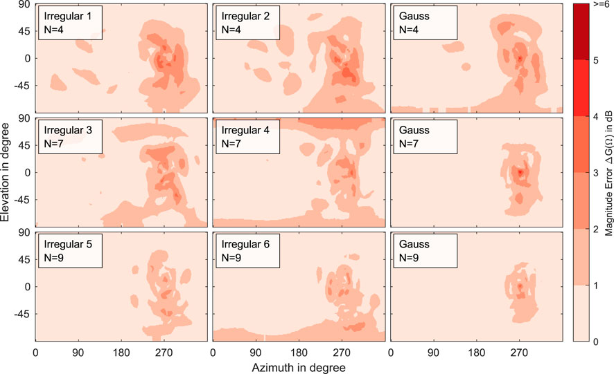
FIGURE 8. Left-ear magnitude error ΔG(Ω) for six examined irregular grids and three regular Gauss grids, with estimated optimal (irregular) or corresponding (regular) SH order. HRTF: Subject no. 10 from HUTUBS database.

4 Discussion

4.1 Interpolation Error Analysis for Different Spherical Harmonics Orders

Investigating the interpolation of sparse irregular HRTF sets with different SH orders revealed a characteristic pattern of the error ΔG with increasing SH order. First, for low orders, the sparsity error decreases. Then, towards the maximum order N_max, the error increases again as the least-squares solution becomes more and more ill-conditioned. As expected, when Tikhonov regularization was applied, an attenuating effect on the numerical instability error was observed. Notably, the regularization showed better results when the regularization value was higher (ϵ = 10^–2) than suggested in other studies (between 10^–8 and 10^–5, see Section 2.4). Since these studies used dense sampling grids and higher SH orders, a comparison is not directly possible. However, based on our results, we assume that for sparse irregular grids, a higher regularization is necessary and appropriate. Pollow et al. (2012) reported that the interpolation result at high frequencies was better when using a lower amount of ϵ = 10^–8 compared to ϵ = 10^–6. However, in our evaluation, we did not find any negative impact of the high regularization amount on the interpolation error. One reason for this could be that in our case, the sparsity error caused by the low SH orders is much more dominant than the error introduced by regularization. Only for regularization values higher than 10⁻², as shown in the Supplementary Figures S5–S20, the interpolation error increases notably. An in-depth study on regularization of sparse grids, ideally with an emphasis on the numerical properties, should be considered as future work.

The comparison of the interpolation error and the condition number κ for each SH order revealed no clear relation. All examined interpolations were stable up to a condition value of κ < 10. However, even with a comparably high value, this would be a rather conservative stability criterion, as in some cases even considerably higher condition values still lead to stable results. Overall, our results suggest that, at least for irregular grids, the upper bound on stability is more relaxed than the commonly used value of κ = 3.5 (Ben-Hur et al., 2019; Ackermann et al., 2021).

4.2 Estimation of Optimal Spherical Harmonics Order

With the interpolation error analysis, we intended to find a perceptually motivated method to derive the optimal SH order for irregular sparse HRTF sets. As shown in Section 3.2, the condition number κ seems not to be the best measure to derive the optimal SH order, especially when working with irregular grids. However, evaluation of the interpolation error for the test HRTF sets revealed a characteristic error curve. Hence, instead of the condition number κ, the SH order with the smallest associated magnitude error ΔG can be considered as the optimal SH order for the particular sampling grid. Our evaluation showed that this method provides reliable results, but it requires a dense reference HRTF set for evaluating the magnitude error. For this reason, we repeated the interpolation error analysis for various HRTF databases and found that, when using the same test grid, the estimated optimal SH order is almost always the same for all examined HRTF databases.

Based on these results, we propose to determine the optimal SH order for sparse irregular grids based on the interpolation error across SH order for a reference HRTF set resampled to the respective sparse irregular grid. As for the reference HRTF set a dense representation is available, the interpolation error can be calculated for any possible sparse irregular grid. Although this method relies on the rather time-consuming calculation of several interpolations and is therefore quite unsuitable for real-time application, it provides a much more reliable estimate of the required optimal SH order than approximation based on the condition number κ. In general, there might be other, possibly more accurate, analytical methods in linear algebra for such problems. However, we argue that the error metric used in the present work provides better SH order estimates regarding perceptual quality than purely analytical methods that only consider the sampling scheme without including the actual HRTF data. For future work, a combination of the proposed perceptually motivated method and an analytical approach could be of great interest to further improve the SH order estimation. Furthermore, other HRTF error metrics could be considered, such as auditory models as recently used by Engel et al. (2022). It should be mentioned that all of the grids used in this evaluation were obtained during actual measurements with uniform spherical sampling in mind. Thus, this evaluation does not consider extreme cases, such as large holes or an overly imbalanced distribution of points.

Finally, we compared the interpolations of the six examined irregular HRTF sets with optimal SH order to the interpolation of regular HRTF sets (Gauss grids) with corresponding SH order. This comparison verified the proposed method for estimating the optimal SH order and put the results into context of interpolation studies of regular sparse grids, such as Ben-Hur et al. (2019) or Arend et al. (2021). For comparable orders, the interpolation results found in the present study for irregular grids are very similar to those found for regular grids in Arend et al. (2021).

We would like to emphasize that the proposed method can be used not only with the HRTF preprocessing method applied in this work, i.e., SUpDEq and Tikhonov regularization, but also with any preprocessing method for SH-based HRTF interpolation. The estimated SH order is then optimal for the respective chosen method. A further generalization to data other than HRTFs, e.g., loudspeaker or voice directivity patterns, could be examined in future research.

5 Conclusion

In this study, we investigated the SH interpolation of HRTF sets sampled on sparse irregular grids. We found that Tikhonov regularization, even at high regularization strength, generally has a positive effect on SH interpolation of irregularly sampled HRTFs and does not increase the interpolation error when applied with high regularization amount, as is often the case with regular (dense) grids. Furthermore, we showed that determining the optimal SH order for interpolation cannot be directly derived from the sampling grid and the associated condition number κ. As a more reliable alternative approach, we proposed a method to estimate the optimal SH order for interpolating sparse irregular HRTF measurements based on the order-dependent magnitude error for a reference HRTF set. A final comparison of the interpolation errors for irregular and regular HRTF sets showed good performance of the estimation method. The proposed method and the insights gained on SH interpolation of HRTFs sampled on sparse irregular grids are of great value for new approaches to individual HRTF measurements, such as FBM systems.

Data availability statement

The original contributions presented in the study are included in the article/Supplementary Material, further inquiries can be directed to the corresponding author.

Author contributions

All authors contributed to the conceptual idea and method. DB performed the investigation, software implementation, visualization, and writing of the original draft. JA and CP contributed to the original draft, reviewed and edited the manuscript, and supervised the work. All authors read and approved the final manuscript.

Funding

This work has been carried out within the research project RESKUe, funded by the BMWi (Federal Ministry for Economic Affairs and Energy) under the funding reference code 03THWO9K07.

Acknowledgments

We would like to thank the participants of the HRTF measurements conducted with our FBM system, from which we obtained the irregular test sampling grids. We would also like to thank all reviewers for taking the time and effort to review the manuscript. We are grateful for the valuable comments and suggestions that helped us to improve the quality of the manuscript.

Conflict of Interest

The authors declare that the research was conducted in the absence of any commercial or financial relationships that could be construed as a potential conflict of interest.

Publisher’s Note

All claims expressed in this article are solely those of the authors and do not necessarily represent those of their affiliated organizations, or those of the publisher, the editors and the reviewers. Any product that may be evaluated in this article, or claim that may be made by its manufacturer, is not guaranteed or endorsed by the publisher.

Supplementary material

The Supplementary Material for this article can be found online at: https://www.frontiersin.org/articles/10.3389/frsip.2022.884541/full#supplementary-material

References

Ackermann, D., Brinkmann, F., Zotter, F., Kob, M., and Weinzierl, S. (2021). Comparative evaluation of interpolation methods for the directivity of musical instruments. Audio Speech Music process., 36–14. doi:10.1186/s13636-021-00223-6

CrossRef Full Text | Google Scholar

Ahrens, J., Thomas, M. R. P., and Tashev, I. (2012). “HRTF magnitude modeling using a non-regularized least-squares fit of spherical harmonics coefficients on incomplete data,” in Proceedings of the Asia-Pacific Signal and Information Processing Association Annual Summit and Conference, December 03-06, 2012 (Hollywood, CA: IEEE) 1–5.

Google Scholar

Andreopoulou, A., and Katz, B. F. G. (2017). Identification of perceptually relevant methods of inter-aural time difference estimation. J. Acoust. Soc. Am. 142, 588–598. doi:10.1121/1.4996457

PubMed Abstract | CrossRef Full Text | Google Scholar

Arend, J. M., Brinkmann, F., and Pörschmann, C. (2021). Assessing spherical harmonics interpolation of time-aligned head-related transfer functions. J. Audio Eng. Soc. 69, 104–117. doi:10.17743/jaes.2020.0070

CrossRef Full Text | Google Scholar

Arend, J. M., and Pörschmann, C. (2019). “Spatial upsampling of sparse head-related transfer function sets by directional equalization - influence of the spherical sampling scheme,” in in Proceedings of the 23rd International Congress on Acoustics (ICA), September 9–13, 2019 (Aachen, Germany: Deutsche Gesellschaft für Akustik (DEGA)), 2643–2650. doi:10.18154/RWTH-CONV-238939

CrossRef Full Text | Google Scholar

Bau, D., Lübeck, T., Arend, J. M., Dziwis, D. T., and Pörschmann, C. (2021). “Simplifying head-related transfer function measurements: A system for use in regular rooms based on free head movements,” in Proceedings of the International Conference on Immersive and 3D Audio (I3DA), September 08-10, 2021 (Bologna, Italy: IEEE), 1–6. doi:10.1109/I3DA48870.2021.9610890

CrossRef Full Text | Google Scholar

Bau, D., and Pörschmann, C. (2022). “Technical Evaluation of an Easy-To-Use Head-Related Transfer Function Measurement System,” in Proceedings of the 48th DAGA, March 21–24, 2022 (Stuttgart, Germany: Deutsche Gesellschaft für Akustik (DEGA)), 367–370.

Google Scholar

Ben-Hur, Z., Alon, D. L., Rafaely, B., and Mehra, R. (2019). Loudness stability of binaural sound with spherical harmonic representation of sparse head-related transfer functions. EURASIP J. Audio Speech Music Process. 2019, 5. doi:10.1186/s13636-019-0148-x

CrossRef Full Text | Google Scholar

Bernschütz, B. (2013). “A spherical far field HRIR/HRTF compilation of the Neumann KU 100,” in Proceedings of the 39th DAGA, March 18–21, 2013. Merano, Italy: DEGA, 592–595.

Google Scholar

Bernschütz, B., Giner, A. V., Pörschmann, C., and Arend, J. M. (2014). Binaural reproduction of plane waves with reduced modal order. Acta Acust. United Acust. 100, 972–983. doi:10.3813/AAA.918777

CrossRef Full Text | Google Scholar

Bomhardt, R. (2017). Anthropometric Individualization of Head-Related Transfer Functions. RWTH Aachen.

Braren, H., and Fels, J. (2020). A high-resolution head-related transfer function data set and 3D-scan of KEMAR. doi:10.18154/RWTH-2020-11307

CrossRef Full Text | Google Scholar

Brinkmann, F., Dinakaran, M., Pelzer, R., Grosche, P., Voss, D., and Weinzierl, S. (2019). A cross-evaluated database of measured and simulated HRTFs including 3D head meshes, anthropometric features, and headphone impulse responses. J. Audio Eng. Soc. 67, 705–718. doi:10.17743/jaes.2019.0024

CrossRef Full Text | Google Scholar

Brinkmann, F., Lindau, A., Weinzierl, S., van der Par, S., Müller-Trapet, M., Opdam, R., et al. (2017). A high resolution and full-spherical head-related transfer function database for different head-above-torso orientations. J. Audio Eng. Soc. 65, 841–848. doi:10.17743/jaes.2017.0033

CrossRef Full Text | Google Scholar

Chen, J., Van Veen, B. D., and Hecox, K. E. (1995). A spatial feature extraction and regularization model for the head-related transfer function. J. Acoust. Soc. Am. 97, 439–452. doi:10.1121/1.413110

PubMed Abstract | CrossRef Full Text | Google Scholar

Demmel, J. W. (1997). Linear least squares problems. Appl. Numer. Linear Algebra Soc. Industrial Appl. Math. 3, 101. –138. doi:10.1137/1.9781611971446.ch3

CrossRef Full Text | Google Scholar

Djelani, T., Pörschmann, C., Sahrhage, J., and Blauert, J. (2000). An interactive virtual-environment generator for psychoacoustic research II: Collection of head-related impulse responses and evaluation of auditory localization. Acta Acustica united Acustica 86, 1046–1053.

Google Scholar

Duraiswami, R., Zotkin, D. N., and Gumerov, N. A. (2004). “Interpolation and range extrapolation of HRTFs,” in IEEE International Conference on Acoustics, Speech, and Signal Processing, May 17–21, 2004 (Montreal, QC: IEEE), 45–48.

Google Scholar

Engel, I., Goodman, D. F. M., and Picinali, L. (2022). Assessing HRTF preprocessing methods for Ambisonics rendering through perceptual models. Acta Acust. 6. doi:10.1051/aacus/2021055

CrossRef Full Text | Google Scholar

Enzner, G. (2008). “Analysis and optimal control of LMS-type adaptive filtering for continuous-azimuth acquisition of head related impulse responses,” in IEEE International Conference on Acoustics, Speech, and Signal Processing, March 31–April 4, 2008 (Los Angeles, NV: IEEE) 393. doi:10.1109/ICASSP.2008.4517629

CrossRef Full Text | Google Scholar

Enzner, G., Antweiler, C., and Spors, S. (2013). Trends in acquisition of individual head-related transfer functions. Berlin, Heidelberg: Springer Berlin Heidelberg. chap. 3. 57–92. doi:10.1007/978-3-642-37762-4_3

CrossRef Full Text | Google Scholar

Evans, M. J., Angus, J. A. S., and Tew, A. I. (1998). Analyzing head-related transfer function measurements using surface spherical harmonics. J. Acoust. Soc. Am. 104, 2400–2411. doi:10.1121/1.423749

CrossRef Full Text | Google Scholar

Fallahi, M., Brinkmann, F., and Weinzierl, S. (2015). “Simulation and analysis of measurement techniques for the fast acquisition of head-related transfer functions of head-related transfer functions,” in Proceedings of 41th DAGA, March 16-19, 2015 (Nuremberg, Germany: DAGA), 1107–1110.

Google Scholar

Gamper, H. (2013). Head-related Transfer Function Interpolation in Azimuth, Elevation, and Distance. J. Acoust. Soc. Am. 134, EL547–EL553. doi:10.1121/1.4828983

PubMed Abstract | CrossRef Full Text | Google Scholar

Guezenoc, C., and Seguier, R. (2018). “HRTF Individualization: A Survey,” in 148th Convention of the Audio Engineering Society (New York, NY: AES). doi:10.17743/aesconv.2018.978-1-942220-25-1

CrossRef Full Text | Google Scholar

Hansen, P. (1994). Regularization tools: A matlab package for analysis and solution of discrete ill-posed problems. Numer. Algorithms 6, 1–35. doi:10.1007/bf02149761

CrossRef Full Text | Google Scholar

Hartung, K., Braasch, J., and Sterbing, S. J. (1999). “Comparison of different methods for the interpolation of head-related transfer functions,” in 16th AES Int. Conf. on Spatial Sound Reproduction, April 10–12, 1999 (Rovaniemi, Finland: AES), 319–329.

Google Scholar

He, J., Ranjan, R., Gan, W. S., Chaudhary, N. K., Hai, N. D., and Gupta, R. (2018). Fast continuous measurement of HRTFs with unconstrained head movements for 3D audio. J. Audio Eng. Soc. 66, 884–900. doi:10.17743/jaes.2018.0050

CrossRef Full Text | Google Scholar

Li, S., and Peissig, J. (2017). “Fast estimation of 2D individual HRTFs with arbitrary head movements,” in 22nd Int. Conf. Digital Signal Process. (DSP), August 23–25, 2017 (London, UK: IEEE), 2165. doi:10.1109/ICDSP.2017.8096086

CrossRef Full Text | Google Scholar

Lichtblau, D., and Weisstein, E. W. (2022). Condition number. From MathWorld–A wolfram web resource.

Google Scholar

Majdak, P., Balazs, P., and Laback, B. (2007). Multiple exponential sweep method for fast measurement of head related transfer functions. J. Audio Eng. Soc. 55, 609–615.

Google Scholar

Møller, H., Sørensen, M. F., Jensen, C. B., and Hammershøi, D. (1996). Binaural technique: Do we need individual recordings? J. Audio Eng. Soc. 44, 451–469.

Google Scholar

Mossop, J. E., and Culling, J. F. (1998). Lateralization of large interaural delays. J. Acoust. Soc. Am. 104, 1574–1579. doi:10.1121/1.424369

PubMed Abstract | CrossRef Full Text | Google Scholar

Pike, C. W. (2019). Evaluating the perceived quality of binaural technology. York UK: PhD Thesis.

Google Scholar

Pollack, K., and Majdak, P. (2021). “Evaluation of a Parametric Pinna Model for the Calculation of Head-Related Transfer Functions,” in Proceedings of the International Conference on Immersive and 3D Audio (I3DA) (Bologna, Italy: IEEE). doi:10.1109/I3DA48870.2021.9610885

CrossRef Full Text | Google Scholar

Pollow, M., Nguyen, K. V., Warusfel, O., Carpentier, T., Müller-Trapet, M., Vorländer, M., et al. (2012). Calculation of head-related transfer functions for arbitrary field points using spherical harmonics decomposition. Acta Acustica united Acustica 98, 72–82. doi:10.3813/AAA.918493

CrossRef Full Text | Google Scholar

Pörschmann, C., Arend, J., Bau, D., and Lübeck, T. (2020). Comparison of Spherical Harmonics and Nearest-Neighbor based Interpolation of Head-Related Transfer Functions. J. Audio Eng. Soc. doi:10.1016/s0967-2109(00)00016-8

CrossRef Full Text | Google Scholar

Pörschmann, C., Arend, J. M., and Brinkmann, F. (2019a). Directional equalization of sparse head-related transfer function sets for spatial upsampling. IEEE/ACM Trans. Audio Speech Lang. Process. 27, 1060–1071. doi:10.1109/TASLP.2019.2908057

CrossRef Full Text | Google Scholar

Pörschmann, C., Arend, J. M., and Gillioz, R. (2019b). “How wearing headgear affects measured head-related transfer functions,” in Proc. EAA Spatial Audio Signal Process. Symposium, September 6–7, 2019 (Paris, France: EAA), 49–54. doi:10.25836/sasp.2019.27

CrossRef Full Text | Google Scholar

Pörschmann, C., and Arend, J. M. (2019a). “How positioning inaccuracies influence the spatial upsampling of sparse head-related transfer function sets,” in Proc. Int. Conf. Spatial Audio - ICSA, September 26–28, 2019 (Ilmenau, Germany: DEGA) 2019, 1–8.

Google Scholar

Pörschmann, C., and Arend, J. M. (2019b). “Obtaining dense HRTF sets from sparse measurements in reverberant environments,” in Proceedings of the AES international conference on immersive and interactive Audio, March 27–29, 2019 (York, UK: AES), 1–10.

Google Scholar

Rafaely, B. (2005). Analysis and design of spherical microphone arrays. IEEE Trans. Speech Audio Process. 13, 135–143. doi:10.1109/TSA.2004.839244

CrossRef Full Text | Google Scholar

Rafaely, B., and Avni, A. (2010). Interaural cross correlation in a sound field represented by spherical harmonics. J. Acoust. Soc. Am. 127, 823–828. doi:10.1121/1.3278605

PubMed Abstract | CrossRef Full Text | Google Scholar

Rafaely, B. (2015). Fundamentals of spherical array processing. New York: Springer Topics in Signal Processing.

Google Scholar

Reddy, C. S., and Hegde, R. M. (2017). On the conditioning of the spherical harmonic matrix for spatial Audio applications, 1–12.

Google Scholar

Reijniers, J., Partoens, B., Steckel, J., and Peremans, H. (2020). HRTF measurement by means of unsupervised head movements with respect to a single fixed speaker. IEEE Access 8, 1–92300. doi:10.1109/ACCESS.2020.2994932

CrossRef Full Text | Google Scholar

Richter, J.-G. (2019). Fast measurement of individual head-related transfer functions. Dr. Diss. RWTH Aachen. doi:10.30819/4906

CrossRef Full Text | Google Scholar

Richter, J.-G., and Fels, J. (2019). On the influence of continuous subject rotation during high-resolution head-related transfer function measurements. IEEE/ACM Trans. Audio Speech Lang. Process. 27, 730–741. doi:10.1109/TASLP.2019.2894329

CrossRef Full Text | Google Scholar

Romigh, G. D., Brungart, D. S., Stern, R. M., and Simpson, B. D. (2015). Efficient real spherical harmonic representation of head-related transfer functions. IEEE J. Sel. Top. Signal Process. 9, 921–930. doi:10.1109/JSTSP.2015.2421876

CrossRef Full Text | Google Scholar

Shirley, P., and Marschner, S. (2009). Fundamentals of computer graphics. 3 edn. Florida: CRC Press.

Google Scholar

Sibson, R. (1981). “A brief description of natural neighbor interpolation,” in Interpreting multivariate data (John Wiley & Sons), 21–36.

Google Scholar

Slaney, M. (1998). Auditory toolbox: A matlab toolbox for auditory modeling work. Interval Res. Corp. Tech. Rep 10, 1998.

Google Scholar

Tikhonov, A., Goncharsky, A., Stepanov, V., and Yagola, A. G. (1995). Numerical methods for the solution of ill-posed problems. Dordrecht: Springer. doi:10.1007/978-94-015-8480-7

CrossRef Full Text | Google Scholar

Vorländer, M. (2008). Auralization. edn. New York: Springer Berlin Heidelberg, 1. doi:10.1007/978-3-540-48830-9

CrossRef Full Text | Google Scholar

Wenzel, E. M., Arruda, M., Kistler, D. J., and Wightman, F. L. (1993). Localization using nonindividualized head-related transfer functions. J. Acoust. Soc. Am. 94, 111–123. doi:10.1121/1.407089

PubMed Abstract | CrossRef Full Text | Google Scholar

Wenzel, E. M., and Foster, S. H. (1993). “Perceptual consequences of interpolating head-related transfer functions during spatial synthesis,”. Proc. IEEE Workshop Appl. Signal Process. Audio Acoust, October 17–20, 1993 (New Paltz, NY: IEEE), 102–105. doi:10.1109/ASPAA.1993.379986

CrossRef Full Text | Google Scholar

Zhang, W., Abhayapala, T. D., Kennedy, R. A., and Duraiswami, R. (2010). Insights into head-related transfer function: Spatial dimensionality and continuous representation. J. Acoust. Soc. Am. 127, 2347–2357. doi:10.1121/1.3336399

PubMed Abstract | CrossRef Full Text | Google Scholar

Zotkin, D. N., Duraiswami, R., and Gumerov, N. A. (2009). “Regularized HRTF fitting using spherical harmonics,“ in IEEE Workshop on Applications of Signal Processing to Audio and Acoustics, October 18–21, 2009 (New Paltz, NY: IEEE), 257, doi:10.1109/ASPAA.2009.5346521

CrossRef Full Text | Google Scholar

Zotter, F. (2009a). “Analysis and synthesis of sound-radiation with spherical arrays,” (IEM, Univ. Musik u. darstellende Kunst Graz). PhD thesis.192

Google Scholar

Zotter, F. (2009b). “Sampling strategies for acoustic holography/holophony on the sphere sampling characterization,” in International Conference on Acoustics NAG/DAGA, March 23–26, 2009 (Rotterdam, Netherlands: DAGA), 1107–1110.

Google Scholar