Using hyperspectral imaging to identify and classify large microplastic contamination in industrial composting processes

1 Introduction

Microplastics have become a significant environmental concern. They are defined by ISO 2020 standards as solid plastic particles insoluble in water, spanning dimensions between 1 μm and 1,000 μm (1 mm). Large microplastics, are categorized as microplastics spanning dimensions between 1 mm and 5 mm. Typically, a large microplastic object represents an article consisting of plastic or a part of an end-user product or a fragment of the respective article (ISO2020, 2020). They accumulate in various ecosystems, including oceans, rivers, soil, and even the air, due to the widespread usage and slow degradation of plastic products (Tian et al., 2022). There are many routes by which microplastics reach the environment. Typically, food waste is gathered at its source using plastic bags and then transferred to Anaerobic Digestion (AD) plants. The pre-treatment of food waste becomes essential for effectively separating plastics from organic matter, employing mechanical methods like shredders. However, there is a lack of adequate technologies to guarantee the thorough separation of plastic fragments from food waste within AD plants. Consequently, substantial quantities of plastic enter into the AD system, resulting in a significant presence of microplastics (MPs) in the digestate (Manu et al., 2023). Another route is via compost from an industrial composter (IC). Currently there are preventative measures in place used by ICs to minimize this problem and industry standards to ensure the high quality of digestate and compost. In the UK these are covered by the PAS 100 certification (PAS100, 2022).

Microplastics can end up in compost through the contamination of organic waste materials during the composting process (Vithanage et al., 2021). Plastic debris, in the form of small fragments or particles, can unintentionally mix with organic matter which lead to microplastic contamination in the resulting compost (EEA, 2020). Biodegradable and compostable plastics, although designed to degrade more rapidly than conventional (non-compostable) plastics, may not fully break down during composting, resulting in the formation of microplastics (Corcoran, 2022). Additionally, certain products, such as paper cups, plates, or teabags, have thin plastic coatings that can fragment into microplastics during composting if the process is not optimized for their complete degradation. The compost is typically processed to remove all plastics pieces with a size range larger than 5 mm. PAS 100:2018 specifies a physical contaminant upper limit of 0.12% (mass/mass) in the compost (PAS100, 2022).

The presence of microplastics in compost introduces several problems when they enter the environment. Microplastics can alter the physical, chemical, and biological properties of soil, potentially affecting its structure, water retention, nutrient cycling, and microbial activity (De Souza Machado et al., 2019). Furthermore, microplastics can be taken up by plant roots, potentially causing adverse effects on plant growth, development, and overall health. They can also influence the uptake of nutrients and water by plants, and there is a potential risk to human and animal health when microplastic-contaminated compost is applied to agricultural lands (Hu et al., 2022; Tong et al., 2022).

To tackle the microplastic issue requires a comprehensive approach that includes better identification and separation of plastic waste from organic materials, optimizing composting processes for the degradation of compostable and biodegradable plastics (Taneepanichskul et al., 2022).

Various technologies exist for the identification of microplastics in compost samples. Pyrolysis-gas chromatography–mass spectrometry (Py-GC-MS) involves subjecting the compost sample to high temperatures to break down microplastics into their constituent molecules. The resulting vapors are then analyzed using GC–MS to identify and quantify the types of plastic present. Py-GC-MS offers sensitivity, enabling the quantification of nanoplastics even in low quantities. However, a limitation of this technique is the loss of qualitative and quantitative information about the particles, including their number, size, and shape, due to the thermal degradation of the sample (Faltynkova et al., 2021).

To avoid losing morphological information, Py-GC-MS can be combined with other analytical techniques. Raman spectroscopy and Fourier-transform infrared (FT-IR) spectroscopy are optical, non-destructive techniques routinely used for microplastic analysis. Raman spectroscopy can detect particles as small as 1 μm, while FT-IR techniques have a limit of detection of 10–20 μm. These methods can identify the polymer type relatively quickly, but the manual selection of particles can introduce selection bias. Image processing algorithms have been developed to reduce this bias (Xu et al., 2019) although analyzing an entire sample using these techniques can still be time-consuming, complex and expensive (Faltynkova et al., 2021).

HSI has been applied to analyse microplastics and shares many characteristics with FPA-FT-IR spectroscopy. With SWIR-hyperspectral imaging (SWIR-HSI), the entire filter can be captured in a single image using SWIR-HSI camera, eliminating the need for particle selection or the analysis of smaller, discrete areas of the filter. Similar to FPA-FT-IR (Fourier-Transform Infrared) and Raman imaging techniques, HSI produces an image where each pixel corresponds to a spectrum. These spectra can be subjected to multivariate analysis techniques for classification, enabling the identification of chemical signatures associated with objects in the image (Faltynkova et al., 2021). This allows for the visualization of the distribution and concentration of microplastics across the sample surface, providing valuable insights into their spatial characteristics (Bonifazi et al., 2013). Through the use of multivariate techniques, the spectra obtained from each pixel can be classified to identify the chemical signatures associated with different types of microplastics. This allows for the determination of the polymer type, size, number, and shape of the microplastics in the sample (Serranti et al., 2019). The main disadvantage is data size and complexity. HSI generates a large amount of data due to its high spectral and spatial resolution. The acquisition and processing of this data can be computationally intensive and require specialized software and hardware resources. Handling and analyzing such large datasets may pose challenges in terms of storage, processing time, and data management (Taneepanichskul et al., 2022). Moreover, HSI systems typically operate within a specific spectral range, depending on the detectors and filters used. This can limit the ability to analyse certain materials or specific spectral regions of interest. Additional instruments or techniques may be required to cover a broader spectral range, which can add complexity and cost to the analysis setup. HSI provides information about the surface characteristics of the sample but has limited depth resolution. It may therefore not be suitable for analyzing subsurface features or layered structures within the sample (Faltynkova et al., 2021).

The use of HSI technologies have been described in few works for microplastics identification. Karlsson et al. reported that the performance of NIR-HSI is able to detect microplastics with sizes down to 300 μm (Karlsson et al., 2016). Zhao et al. employed VNIR-HSI with spectral range between 400 nm and 1,000 nm to identify PE microplastics (1–5 mm) in soil applying SVM. The detection accuracy for white PE was 84% while the effectiveness dropped to 58% for identifying dark PE (Zhao et al., 2018). Serranti et al. applied SWIR-HSI together with PLS-DA for marine microplastic identification including PP, PE, and PS. The sensitivity and specificity on calibration and cross validation were 1. They found that most common of marine microplastic is PE (Serranti et al., 2018). Zhang et al. (2019) also used NIR-HSI to identify and classify microplastic polymer flakes including PC, PET, PP, PS, and PE with sizes of between 0.1 mm and 1 mm. A support vector machine classification algorithm (SVM) was applied to analyse hyperspectral images in order to classify the different types of polymers (Zhang et al., 2019). Chaczko et al. (2019) used a deep learning method to analyse hyperspectral images for microplastic detection. Around 1,000 samples were used for model training and the model was tested with 100 samples. The results showed that the classification accuracy of the model in a controlled environment was ~95% (Chaczko et al., 2019). Vidal et al. has applied NIR-HSI together with SIMCA to identify 5 polymers including PA-6, PE, PP, PET, and PS in sand. The sensitivity and specificity were more than 99% (Vidal and Pasquini, 2021).

In this paper, we present our work using SWIR-HSI together with PLS-DA to identify large microplastics in compost and to distinguish between compostable large microplastics and non-compostable large microplastics in industrial compost samples. A detailed description of our SWIR-HSI technique is presented, including the hardware and software components. Results are demonstrated at a laboratory scale where we use this method to successfully identify and classify different types of large microplastic (compostable plastics and non-compostable plastics) with high accuracy. We also discuss a SWIR-HSI application using field samples gathered from industrial composters, by showing how our PLS-DA model coped with the task of identifying contaminates plastics obtained from industrial composting facilities.

2 Materials and methods

2.1 Samples collected from industrial composting facility

We visited a commercial composting facility that industrially uses an In Vessel Composting (IVC) method to process mixed food waste and garden waste. This waste contains enters the plant comingled with compostable plastic and non-compostable plastic. Figure 1 details the process steps of the composting process. We collected plastic samples analyzed in this research at step 7.B, which corresponds to the separation of plastics from the compost through sieving using a trommel. A random selection of 50 of these samples were used in this research. We also collected samples of compost from step 8.

Figure 1

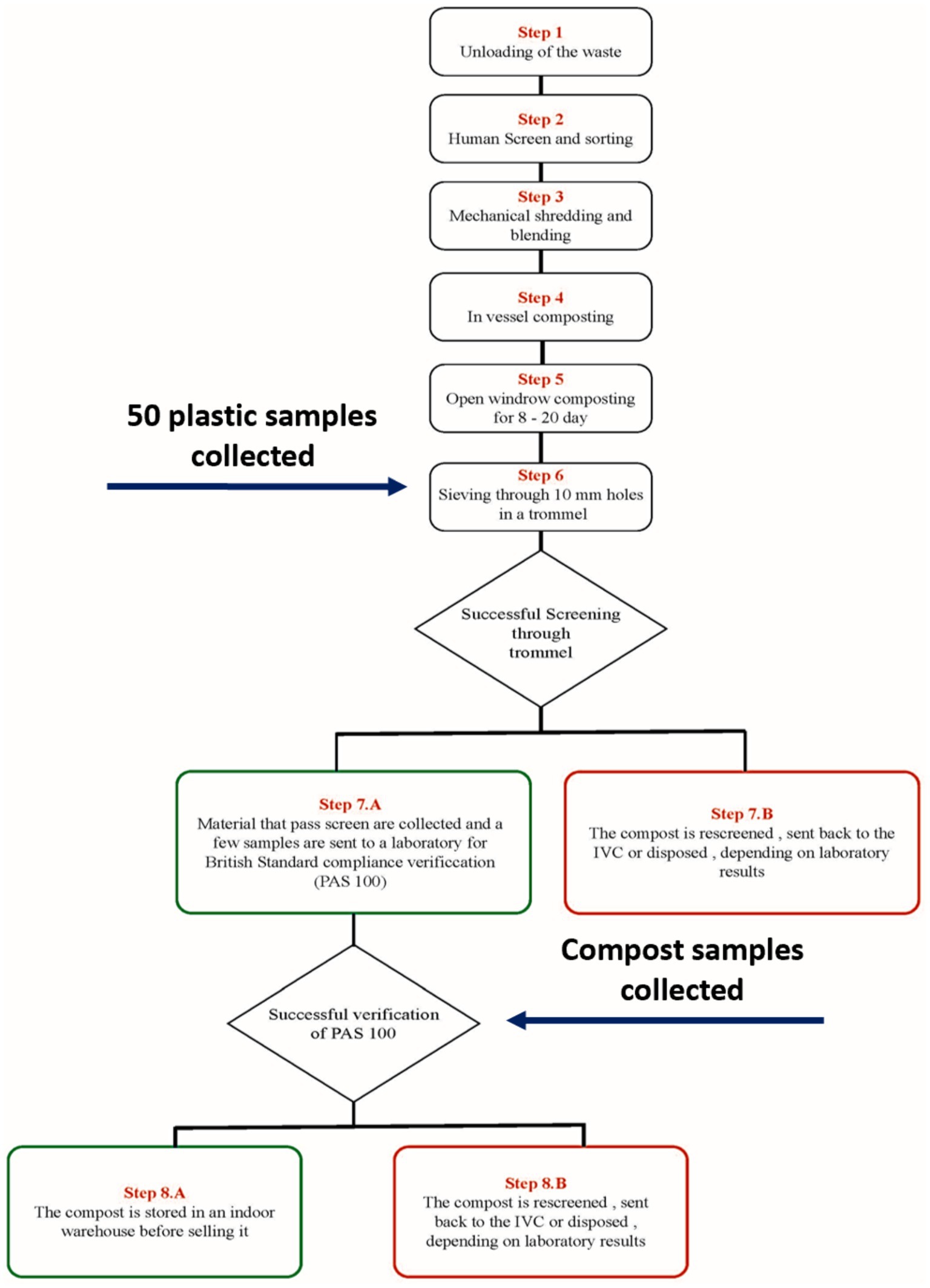
Figure 1. Schematic of the industrial composting process showing the points which samples were collected.

2.2 ATR-FTIR spectroscopy

To validate the classification outcomes obtained from the PLS-DA model using SWIR-HSI data, the 50 unknown plastic samples obtained from the composting plant were identified using a Nicolet^™ iN10 FTIR Microscope. The spectral range investigated spanned from 1,300 to 2,700 nm. The detector employed in this analysis was a liquid nitrogen cooled mercury cadmium telluride detector, while Germanium served as the optical material. Prior to conducting the analysis of the spectrum of the 50 plastics collected from composting plant, the OMNIC software libraries were updated. The pre-existing libraries contain over 50 conventional (non-compostable) polymers but lack presentation of compostable polymers. Hence, PBAT, PLA, and PHA spectra were imported into OMNIC’s libraries. A pre-processing method called “automatic smooth” was initially applied to the sample spectra to mitigate noise. Subsequently, a comparison was made between the spectra of known plastics and the processed sample spectra and identify the 50 samples of plastic from the composting plant.

2.3 Material property evaluation

Multiple characteristics of the 50 plastic samples obtained from the composting plant were examined to determine their darkness, size, color, thickness, and contamination level (see Figure 2). Precise evaluation of the darkness, size and contamination level necessitates the utilization of computer vision algorithms. These algorithms enable advanced analysis and quantitative assessment of the characteristics, ensuring scientific rigor and enhancing the reliability of the measurements.

Figure 2

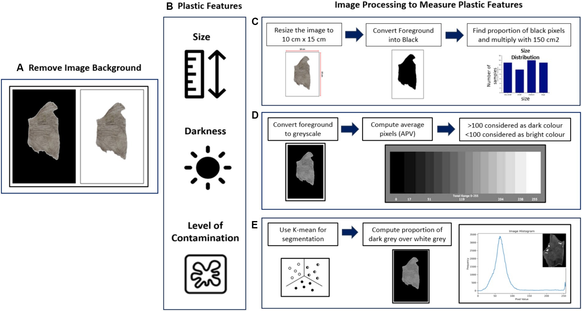
Figure 2. Showing how the 50 plastic samples collected from the trommel separation were characterized using computer vision algorithms: (A) Photographed and background removed; (B) showing how the digital image is processed to determine size, darkness and level of contamination; (C) sequence of image processing used to measure size; (D) sequence of image processing used to measure darkness level; (E) sequence of image processing used to measure level of contamination.

2.3.1 Size and darkness estimation algorithm

The 50 pictures of plastic samples were taken in a photobooth to standardize the lighting conditions. Subsequently, the images were resized to 15 cm × 10 cm as shown in Figure 2. The images were loaded and converted into grayscale. Subsequently, Otsu’s thresholding method (OpenCV, 2023) was applied to convert the grayscale images into binary images or binary masks. Pixels with values below the determined threshold were assigned a value of 0, while pixels above the threshold were assigned a value of 255. This step effectively separated the foreground from the background by identifying the contours of the images. The area of each plastic sample was determined by multiplying the percentage of the plastic area (foreground) by the size of the frame, which was 150 cm². Subsequently, the average pixel value (APV) was computed to quantify the darkness level. This measurement provides an indication of the overall intensity or darkness of the plastic samples.

2.3.2 Level of contamination estimation algorithm

An unsupervised machine learning algorithm, K-means clustering, was utilized to quantify sample contamination, particularly focusing on the presence of attached soil on plastic samples. In the context of image clustering, K-means proves valuable for grouping pixels based on their similarity in color or intensity. Each pixel within a sample image was represented as a feature vector, encompassing its grayscale intensity. To establish the initial cluster configurations, the centroids, serving as the center points of each cluster, were randomly initialized. For each pixel in the image, a similarity measure was calculated to determine its proximity to each of the cluster centroids, utilizing a distance metric such as the Euclidean distance. Based on this calculation, the pixel was assigned to the cluster with the closest centroid, thereby creating the initial clusters. Following the initial assignment, the algorithm proceeded to iteratively update the cluster centroids and reassign pixels until convergence was achieved. In each iteration, pixels were reassigned to the cluster with the nearest centroid, and the centroids were recalculated by taking the mean of all pixel values within their respective clusters. This process continued until the centroids stabilized, signifying minimal change in the pixel assignments. Upon convergence, the algorithm produced the final clustering result. These centroids effectively represented the distinctive characteristics or greyscale intensities per sample that defined each cluster. After this image segmentation, the level of contamination was calculated. The cluster with the lowest mean grayscale value within the plastic sample (foreground) was identified. This specific cluster represented the region with the least intensity and was assumed to correspond to the contamination or non-plastic elements present (see Figure 2). To estimate the proportion of contamination, the ratio of the number of pixels within this cluster to the total number of pixels was computed. This ratio provided an estimate of the contamination level relative to the entire image.

Plastic samples from composting plant varied in size, with the smallest measuring 4.4 cm², the average size being 27.1 cm², and the largest reaching 75.9 cm². The darkness level, assessed by average pixel value (AVP), ranged from 42 to 157, with the darkest sample registering at 42 and the brightest at 157. Most plastic samples had a thickness of less than 2 mm, with the thickest sample measuring 5 mm. Contamination levels varied, with the lowest recorded at 24%, the average at 45%, and the highest at 87.4%. The further detail of plastic samples features will be discussed in section 3.6.

ATR-FTIR was employed to verify the result obtained by PLS-DA classification model. The distribution of samples for each plastic type shows in Figure 3. However, due to a high degree of contamination and the rough surface of some samples, three of them could not be identified.

Figure 3

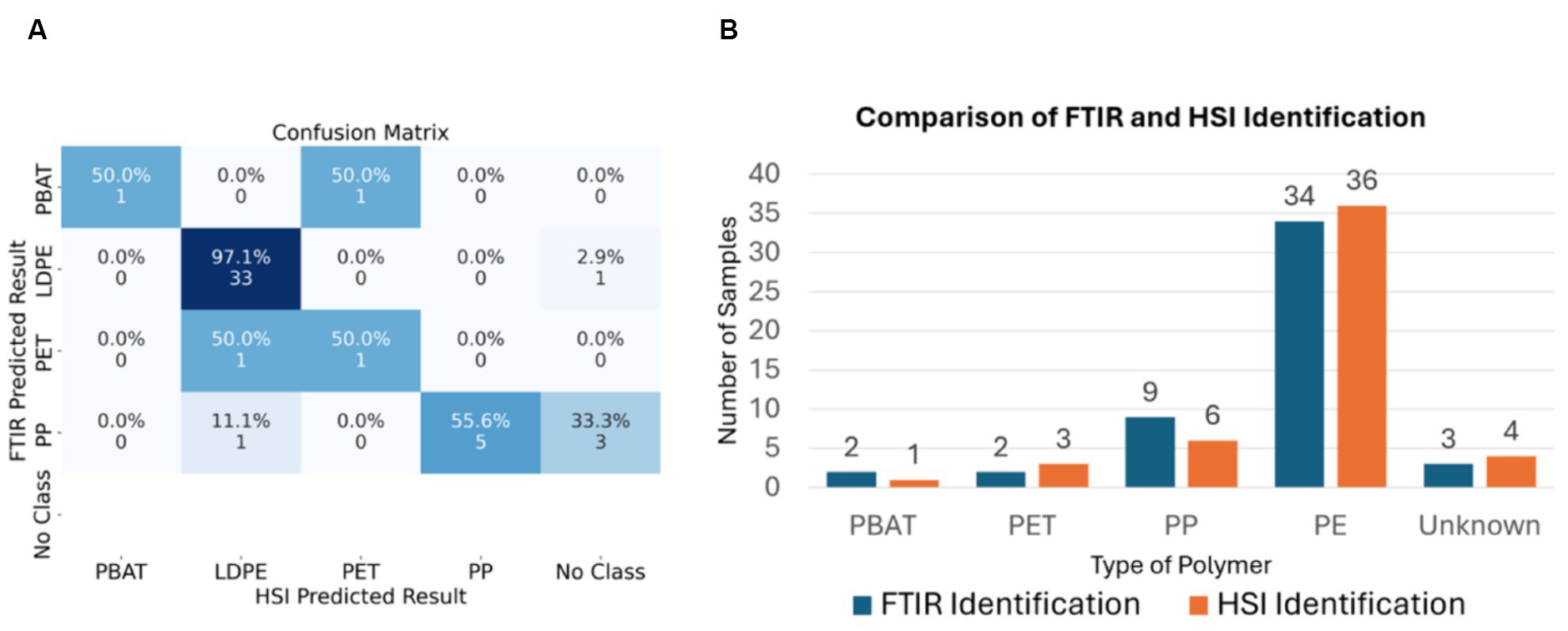
Figure 3. (A) The confusion matrix of FTIR sample prediction and SWIR-HSI sample prediction. (B) Comparison of FTIR and SWIR-HSI field samples identification.

2.4 Hyperspectral imaging system

2.4.1 Materials

Pristine samples of compostable plastics (PLA, PBAT, and PHA) and conventional (non-compostable) plastics (PP, PET, and LDPE) were used to train and test the PLS-DA classification model. The samples were cut into various sizes and divided into two datasets, a training and testing dataset. The size of samples in the training data ranged from 50 mm × 50 mm to 20 mm × 20 mm. While the size of samples in the testing dataset were much smaller—5 mm × 5 mm and samples with diameter from 5 mm to 2 mm. The detail samples dataset including material, sources, type of data, size and number of replicates are shown in Table 1.

Table 1

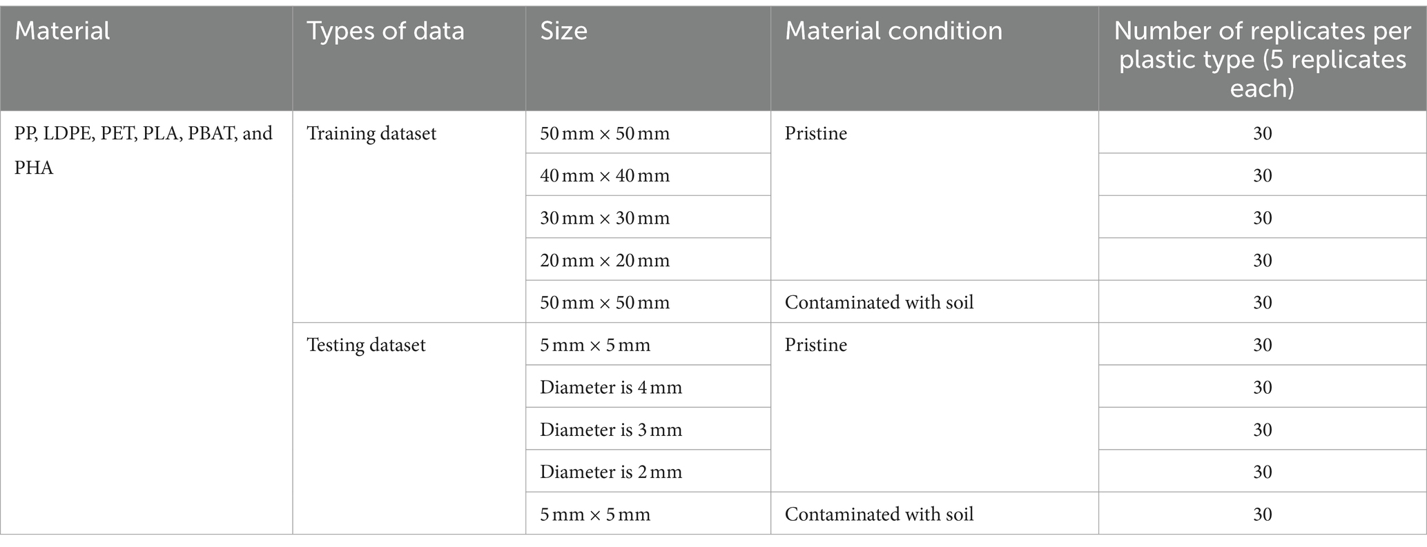
Table 1. The details of samples including materials, types of data, size, material condition, and number of replicates.

2.4.2 Experimental equipment

The hyperspectral Imaging system consists of four main components including a hyperspectral camera, lens, conveyor belt and light source. The height of the SWIR-HSI camera was 100 cm from samples and the angle between the lens and samples was 90°. The halogen lamp was a light source that produced a continuous and intense spectrum from 400 nm to 2,500 nm. We used a conveyor belt (700 mm × 215 mm × 60 mm) as the background for image capture. It was employed to move samples from left to right at an adjustable speed. The geometry of the experimental set-up is shown in our previous work, described in detail in Xiong et al. (2014) and Taneepanichskul et al. (2023). HyspexGround software was used for SWIR-HSI image acquisition, raw absorbance spectra collection and preliminary spectral analysis. A HySpex Baldur S-640iN hyperspectral camera was used to capture both raw absorbance spectra and hyperspectral images. The camera’s spectral range spanned from 950 nm to 1,730 nm, including 232 spectral bands. It operated at a maximum speed of 500 frames per second (fps). Spectral sampling occurred at 3.36 nm intervals, ensuring high-resolution spectral data. The spatial resolution was defined by 640 pixels, facilitating detailed spatial analysis. Lens specifications included a field of view (FOV) of 16° and a corresponding focal length of 282 mm. The camera was configured with a working distance of 1 m, resulting in a spatial size of 0.44 mm (Hyspex, 2019).

The SWIR-HSI data was acquired using a line scan technique. The system produced images in the form of x-y grid of pixel and the spectrum information was recorded for each pixel. The line scans generated a data cube or “hypercube” for each plastic sample.

2.4.3 Spectral preprocessing

Spectral preprocessing has been integrated into chemometrics modeling. The purpose of spectral preprocessing is to remove physical phenomena (artifacts) in the spectra to improve the subsequent multivariate classification model or exploratory analysis (Rinnan et al., 2009). There are many types of spectral preprocessing that have been applied to SWIR spectral data including standard normal variate (SNV), Savistzky-Golay (SG) derivative, smoothing and mean center (MC).

Standard Normal Variate (SNV): SNV is a scattering correction method which is usually applied on spectra where pathlength and baseline changes cause differences between otherwise identical spectra (Rinnan et al., 2009).

Savistzky-Golay (SG) derivative: SG is frequently applied to remove unimportant baseline signals from collected data. This research applied SG as a first derivative filter to highlight the spectral differences with a 15 points window and second polynomial (Cucuzza et al., 2021).

Mean Center (MC): MC is the most common spectral pretreatment method. The data offsets which are not necessary for data variance interpretation are deleted. MC has the effect of including an adjustable intercept in multivariate models (Rinnan et al., 2009).

2.4.4 Principal component analysis

The SWIR range allows the differentiation of types of materials because most absorption bands in this region arise from overtones of C-H, N-H, and O-H vibration which provides chemical information about the material investigated (Serranti et al., 2019). Breeze software version 2022.1.5 was used for spectral data analysis. After a spectral data pre-processing step, principal components analysis (PCA) was applied for an exploratory analysis. PCA is an unsupervised machine learning technique for data dimensionally reduction. PCA decomposes pre-processed spectral data into linear combinations of the original spectral data, namely principle components (PCs). The first PC accounts for the highest variability in the dataset. Hence, most of the information are captured in PC1. The remaining amount of variance become subsequent principal components in descending order (Jolliffe, 2005).

2.4.5 Partial least square and discrimination analysis

Partial Least Squares Discriminant Analysis (PLS-DA) is a supervised machine learning technique that effectively reduces data dimensionality and predicts the class of materials. Combining elements of partial least squares regression (PLS-R) and discriminant analysis (DA), PLS-DA requires an X matrix containing calibration spectra and a corresponding Y matrix specifying the class identity for each set. Typically applied for binary classification, for multiclass scenarios, the Y matrix includes columns equal to the number of classes, forming a dummy matrix with 1’s and 0’s indicating membership or non-membership of a spectrum to a specific class during calibration. The model’s output is not perfectly binary (0 or 1), requiring the establishment of a threshold during prediction (Neves et al., 2022). Various methods exist for setting thresholds, with the application of Bayes’ Theorem being widely accepted (Amigo et al., 2015). Alternatively, a cut-off point of 0.5 is commonly used for binary classification tasks.

In this study, PLS-DA was applied to identify and classify 6 types of materials including PBAT, PLA, PHA, LDPE, PET, and PP and to predict type of polymers in the testing dataset. The samples in training dataset were used to build PLS-DA model. The proper number of latent variables (in this case was 5) were selected for PLS-DA. The linear equation is modeled by latent variables. This allows graphical visualization and an understanding of the relationships by LV scores and loadings (Wold et al., 2001). Subsequently, the model applied to predict sample in testing dataset and measure the performance of model.

2.4.6 PLS-DA performances

To evaluate the classification performance of the PLS-DA classification model, confusion matrices were generated for both the training and testing datasets. These metrics provide a detailed overview of the model’s predictions in comparison to the actual class labels. Beyond the confusion matrix, several key metrics were calculated to assess the effectiveness of the PLS-DA classification model including sensitivity, specificity, F1 score and overall accuracy. Sensitivity measures how well a machine learning model can detect positive instances, defined in Equation (1). Specificity measures the proportion of true negatives that are correctly identified by the model, defined in Equation (2). The F1 score is a metric that represents the harmonic mean of precision and recall (sensitivity), effectively combining these two aspects into a single value. It proves particularly valuable in assessing model performance on imbalanced datasets. The F1 score considers both false positives and false negatives, as illustrated in Equation (3). Accuracy measures the number of correct predictions made by a model in relation to the total number of predictions made, defined in Equation (4) (Kumar, 2022).

$\begin{array}{ll}\mathit{Sensitivity}=\frac{\mathit{True}\mathit{Positive}}{\mathit{True}\mathit{Positive}+\mathit{False}\mathit{Negative}}& (1)\end{array}$

$\begin{array}{ll}\mathit{Specificity}=\frac{\mathit{True}\mathit{Negative}}{\mathit{True}\mathit{Negative}+\mathit{False}\mathit{Positive}}& (2)\end{array}$

$\begin{array}{ll}F1-\mathit{Score}=\frac{\mathit{True}\mathit{positive}}{\mathit{True}\mathit{positive}+\frac{1}{2}\left(\mathit{False}\mathit{Positive}+\mathit{False}\mathit{Negative}\right)}& (3)\end{array}$

$\begin{array}{l}\mathit{Accuracy}=\\ \frac{\mathit{True}\mathit{Negative}+\mathit{True}\mathit{Positive}}{\mathit{True}\mathit{Negative}+\mathit{True}\mathit{Positive}+\mathit{False}\mathit{Negative}+\mathit{False}\mathit{Positive}}\end{array}\text{ (4)}$

The ROC curve, specifically, was employed to visualize the trade-off between the true positive rate (sensitivity) and the false positive rate at various classification thresholds. By analyzing the ROC curve and calculating the AUC, one can gain insights into the discriminatory power of the PLS-DA model and its ability to distinguish between the different classes in the dataset. This graphical representation is especially valuable in binary classification scenarios, providing a comprehensive understanding of the model’s performance across a spectrum of decision thresholds (Hoo et al., 2017).

3 Experimental results

3.1 Average raw absorbance spectrum

The average raw absorbance spectra of PP, PET, LDPE, PLA, PBAT, and PHA is shown in Figure 4A. The SWIR ranges allow polymers to be distinguished because most absorption bands in the spectral region arise from overtone vibrations of molecular bonds between carbon and hydrogen (C-H). The polymer spectra show pronounced different shapes in the ranges 1,150–1,250 nm, 1,350–1,450 nm, and 1,650–1,750 nm. The materials showed different spectral signatures in these regions according to their chemical structure. In order to unambiguously identify the material using these spectra, three spectra pre-processing methods were applied to the raw data:

1. Standard Normal Variate (SNV) + MC (see Figure 4B).

2. Savitzky–Golay (SG) + MC (1st derivative, 2nd polynomial and 15 points window) (see Figure 4C).

3. Savitzky–Golay (SG) (1st derivative, 2nd polynomial and 15 points window) + Standard Normal Variate (SNV) + MC (see Figure 4D).

Figure 4

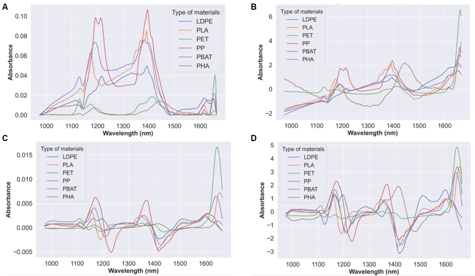
Figure 4. (A) Average raw absorbance spectra of PP, PET, LDPE, PLA, PBAT and PHA and average pre-processed spectra of PP, PET, LDPE, PLA, PBAT, and PHA in SWIR region adopting 3 set of pre-processing methods: (B) SNV + MC; (C) SG (1st derivative, 2nd polynomial and 15-point window) + MC; (D) SG (1st derivative, 2nd polynomial and 15-point window) + SNV + MC.

3.2 The standard normal variate + mean center method

The SNV with a subsequent MC pre-processing method was applied to the raw absorbance spectra, followed by the construction of a PLS-DA score plot. LV1 and LV2 captured 44.2 and 27.4% of the variance, respectively. The clearest distinction between the types of materials clusters was observed in the LV1 vs. LV2 plot, as shown in Figure 5A.

Figure 5

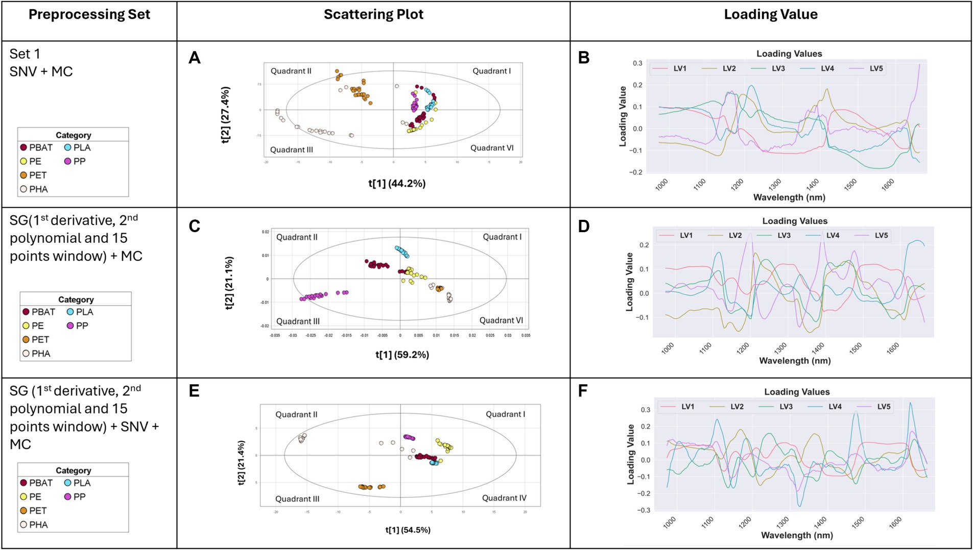
Figure 5. Score variance plot of PLS-DA model with (A) SNV + MC, (C) SG (1st derivative, 2nd polynomial and 15 points window) + MC, and (E) SG (1st derivative, 2nd polynomial and 15 points window) + SNV + MC pre-processing technique; loading score plot of spectra after (B) SNV + MC, (D) SG (1st derivative, 2nd polynomial and 15 points window) + MC, and (F) SG (1st derivative, 2nd polynomial and 15 points window) + SNV + MC pre-processing technique.

Due to their low spectral variance and high uniformity, PET exhibited the highest level of separability, positioning them in the second quadrants, respectively. The scores for PP, LDPE, PLA, and PBAT were localized in the first and fourth quadrants. However, some overlapping was observed between PBAT, PLA, and PE.

From the loading score plot (Figure 5B), the most crucial wavelengths for plastics separation were identified as 1,173–1,223, with a subsequent emphasis on the range from 1,073 to 1,123. These loading scores highlight the significance of these specific wavelengths in the effective separation of plastics.

3.3 The Savitzky–Golay + mean center method

The SG, utilizing a 1st derivative, 2nd polynomial, and a 15-point window followed by mean centering preprocessing method, was employed to preprocess the raw absorbance spectra, followed by PLS-DA classification. The resulting PLS-DA score plot is depicted in Figure 5C. The majority of the variance was effectively captured by the first two components (latent variables), with LV1 and LV2 describing 59.2 and 21.1% of the total variance, respectively.

The class separation among the plastic types is notably robust. PP and PLA demonstrated an exceptionally high level of separability. PHA and PET were localized on fourth quarter. The scores for PBAT and LDPE were predominantly localized centrally positioned in the plot and reveal some overlapping tendencies. In Figure 5D, the loading scores highlight necessary information regarding the optimal wavelengths for plastic separation. The analysis underscores that the most significant range lies between 1,174 and 1,224, with a subsequent range observed from 1,374 to 1,424.

3.4 The combination of Savitzky–Golay method, standard normal variate and mean center

SG utilizing 1st derivative, 2nd polynomial and 15-point window followed by SNV and Mean MC pre-processing method was applied to pre-process the raw spectra. Subsequently, PLS-DA was conducted. The PLS-DA score plot is shown in Figure 5E. LV1 and LV2 accounted for 54.5 and 21.4% of the variance. PET and PHA were located in third and second quadrants respectively, demonstrating a substantial level of separability. The distribution of PP and LDPE scores were localized in the first quadrant with an excellent level of separation. The cluster separation between PBAT and PLA was particularly noticeable in the fourth quadrant. From Figure 5F, the loading scores revealed the crucial wavelength for plastic separation was situated between 1,323 and 1,373, followed by 1,623–1,673.

3.5 Classification of performance

3.5.1 Classification of performance on training dataset

The PLS-DA classification models were used on a training dataset and testing dataset. The sensitivity, specificity, F1 score and overall accuracy of each model were calculated on both datasets and compared to determine the most effective classification model.

The sensitivity, specificity, and F1 for all types of plastic in the training dataset, including LDPE, PLA, PP, PET, PBAT, and PHA, each scored 1 for three PLS-DA classification models with different pre-processing methods (Set 1, Set 2, Set 3). Additionally, the overall accuracy was consistently recorded as 100% across all PLS-DA models with varied pre-processing methods (Set 1, Set 2, Set 3). Figures 6A,B provide a snapshot of the PLS-DA applied to the training dataset. These results imply outstanding performance in identifying plastics larger than 20 mm × 20 mm. Moreover, the classification models demonstrated remarkable capability in accurately identifying plastic types even in the presence of soil contamination (soil on polymer surface), achieving a 100% accuracy rate.

Figure 6

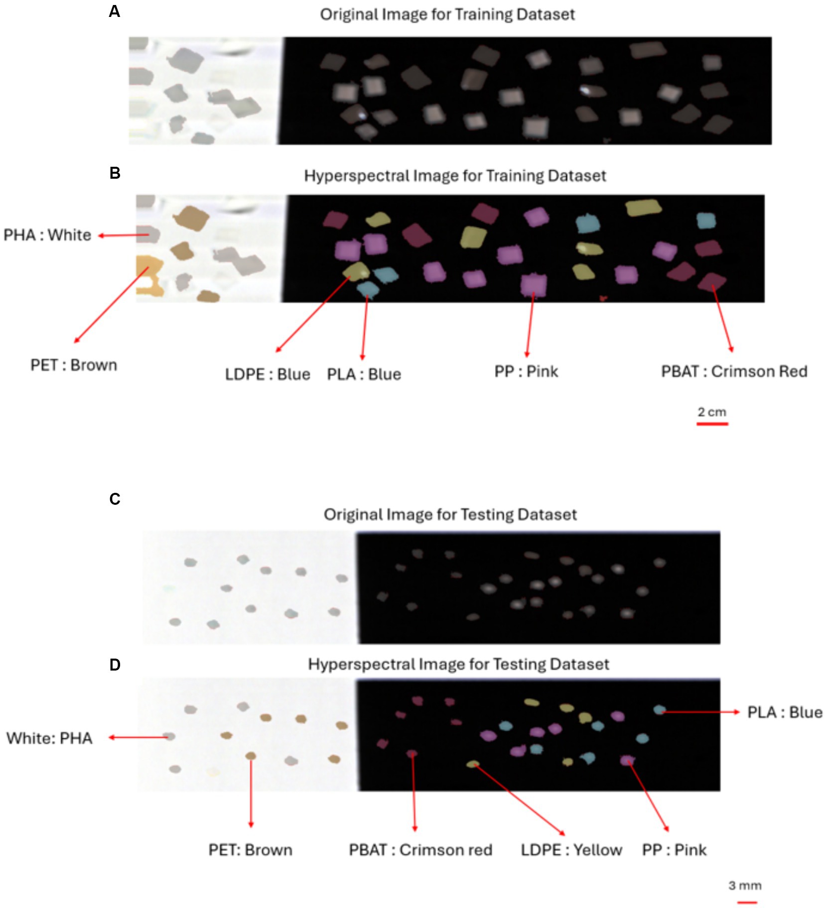
Figure 6. PLS-DA model applied to plastic in training dataset and testing dataset (large microplastic): (A) RGB optical image of plastics in training dataset obtained by the hyperspectral camera; (B) the hyperspectral image plastics in training dataset overlayed with the classification color. (C) RGB optical image of plastics in testing dataset (large microplastics) obtained by the hyperspectral camera (D) the hyperspectral image plastics in testing dataset (large microplastics) overlayed with the classification color.

3.5.2 Classification of performance on testing dataset

The confusion matrix of each classification model was computed. Additionally, the sensitivity, specificity, F1 score and overall accuracy of the classification models were calculated to assess and compare the performance of each model (see Figure 7; Table 2).

Figure 7

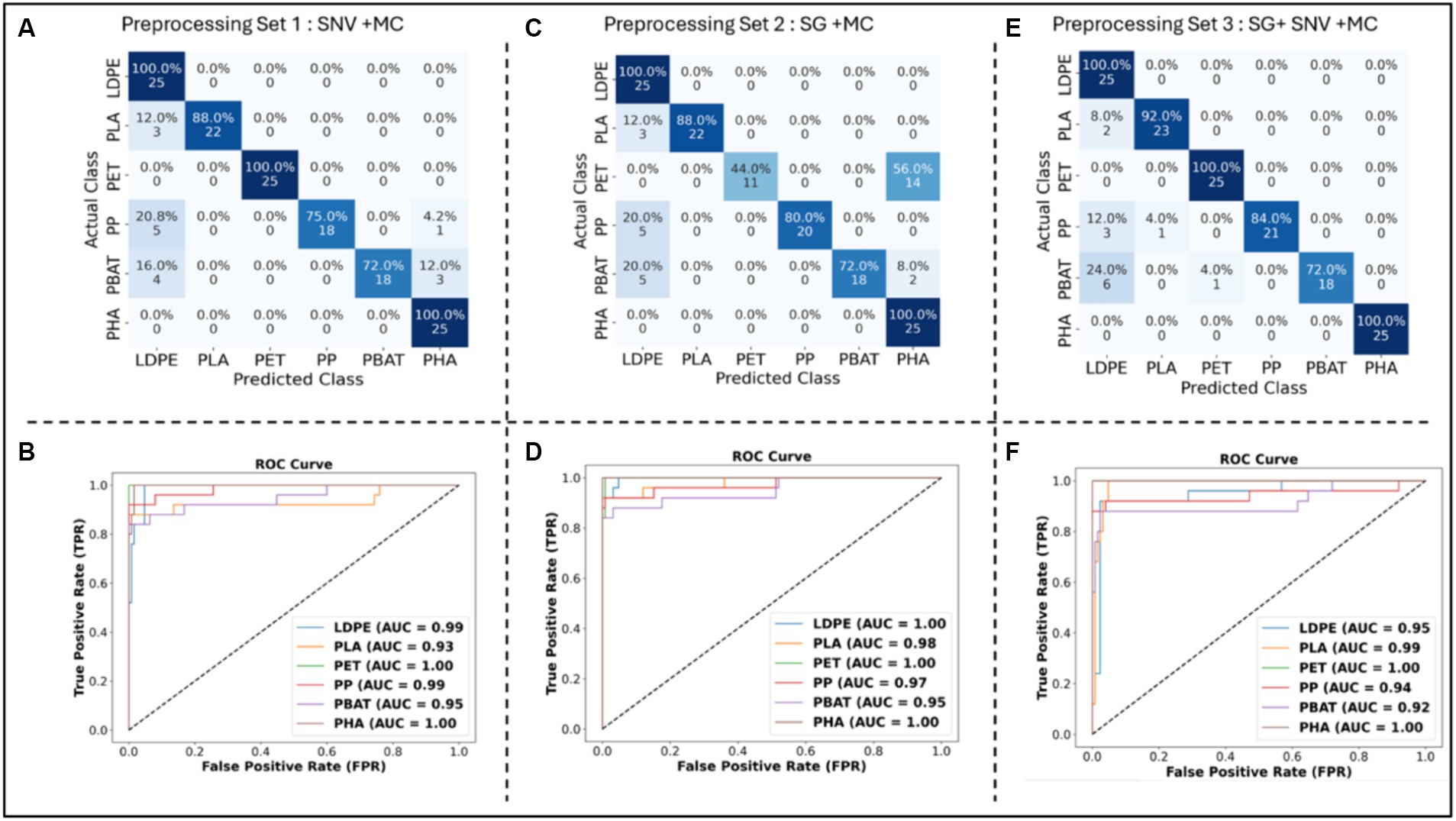
Figure 7. Confusion Matrix of PLS-DA classification models with (A) SNV + MC, (C) SG (1st derivative, 2nd polynomial and 15 points window) + MC, (E) SG (1st derivative, 2nd polynomial and 15 points window) + SNV + MC pre-processing methods; ROC curve of PLS DA classification models with (B) SNV + MC, (D) SG (1st derivative, 2nd polynomial and 15 points window) + MC, and (F) SG (1st derivative, 2nd polynomial and 15 points window) + SNV + MC pre-processing methods applied to the testing dataset.

Table 2

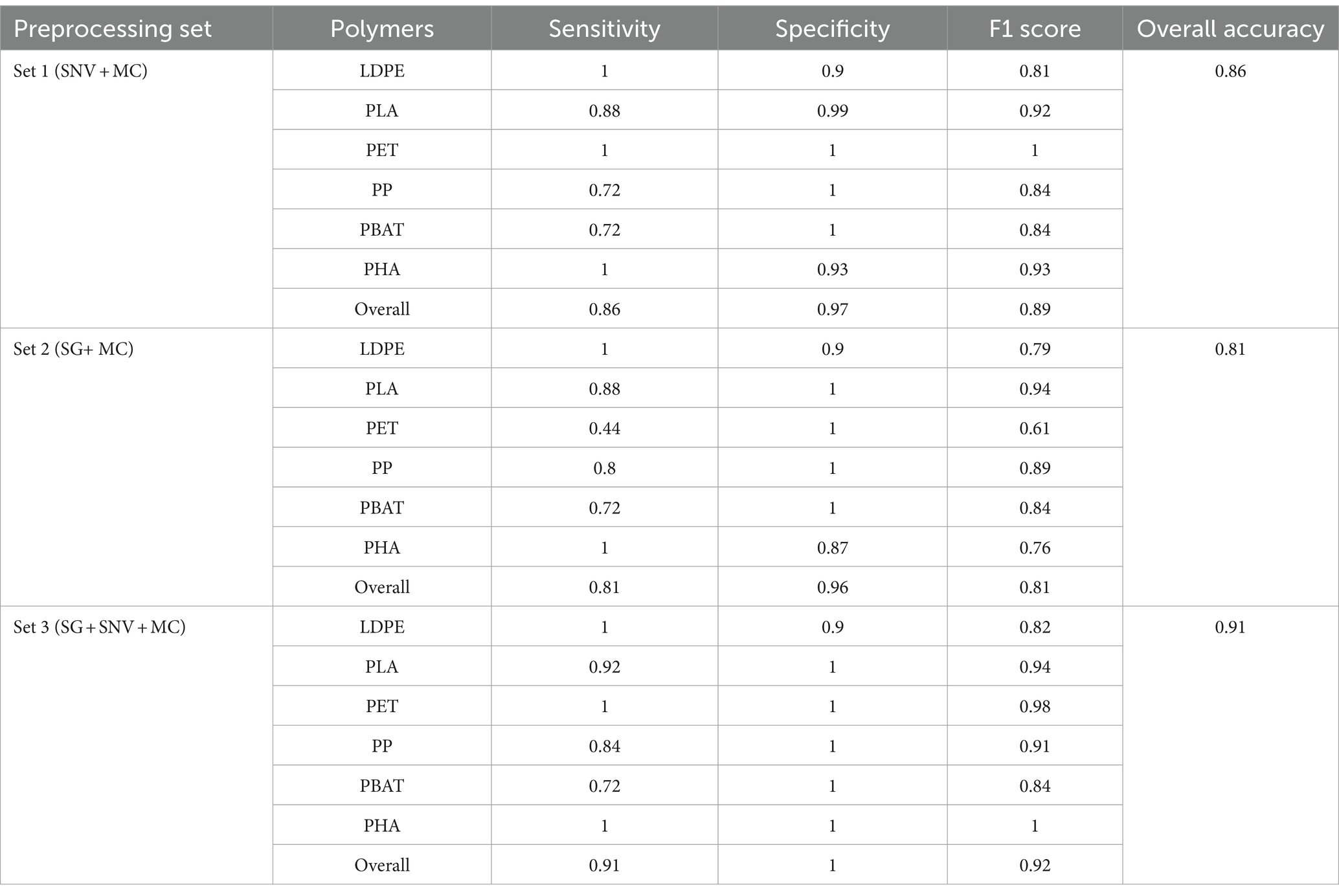
Table 2. Specificity, sensitivity, F1 score and overall accuracy for PLS-DA with different pre-processing methods (set 1, set 2, set 3) on testing dataset.

3.5.2.1 Classification performance of PLS-DA with SNV + MC pre-processing

As shown in Figure 7A, PLS-DA with SNV + MC pre-processing encountered challenges in accurately identifying PP, PBAT, and PLA. Especially, some PP plastics were misclassified as LDPE (20%) or PHA (4%). Specifically, 16% of PBAT plastics were incorrectly classified as LDPE, and 12% were misclassified as PHA. Moreover, for PLA, 12% of instances were inaccurately classified as LDPE. On the other hand, the sensitivity for LDPE, PET, and PHA identification reached 100%. LDPE, PET, PP, PBAT, and PHA exhibited outstanding discriminatory power with AUC values equal to or greater than 95%, whereas PLA demonstrated slightly lower AUC value (see Figure 7B).

In terms of sensitivity, the classification model demonstrates excellent performance by correctly identifying all instances of LDPE, PET, and PHA in the testing dataset (see Table 2). However, the model’s ability to detect PLA, PP, and PBAT is comparatively lower, with sensitivities of 0.88, 0.72, and 0.72, respectively. This suggests that while the model captures LDPE, PET, and PHA, it may have some difficulty identifying instances of PLA, PP, and PBAT, leading to a lower sensitivity for these materials. The ability to correctly identify negative samples (samples which do not belong to the class) of LDPE and PHA were lower than other classes with values of specificity of 0.9 and 0.93, respectively. While specificity of PLA and other classes were 0.99 and 1. The overall performance in terms of both minimizing false positives and false negatives, is indicated by the F1 score. Table 2 shows that LDPE scored the lowest 0.81 followed by PP and PBAT with 0.84. PLA, PHA and PET achieved 0.92, 0.93 and 1, respectively. These F1 scores indicate a strong performance in identifying PLA, PHA, and PET. LDPE, PP, and PBAT exhibit satisfactory performance, although with slightly lower F1 scores.

3.5.2.2 Classification performance of PLS-DA with SG + MC preprocessing

As shown from the confusion matrix (Figure 7C), the classification model faced challenges in correctly identifying PET, PP, and PBAT with misclassification rate 56, 20, and 28%, respectively. A substantial of 56% of PET sample were mistakenly labeled as PHA. While 20% of PP and PBAT was classified as LDPE. However, the model exhibited remarkable accuracy in distinguishing LDPE, PLA, and PHA, achieving high sensitivity in these specific classifications. The testing dataset’s AUC values for all polymers are remarkably high, underscoring the classification model’s strong discriminatory power across the various polymer categories across entire range of threshold values. The ROC curve analysis revealed an exceptionally high discriminating power for all types of polymers across the threshold range (Figure 7D).

The sensitivity of LDPE and PHA reached an high value of 1, surpassing that of PLA and PP (0.88 and 0.8, respectively) (see Table 2). Nevertheless, the model struggled to identify accurately PBAT and PET, resulting in a significant drop in sensitivity to 0.72 and 0.44, respectively. In terms of specificity, LDPE and PHA demonstrated the lowest values, indicating difficulties in the model’s ability to correctly identify plastic samples that did not belong to their respective classes. 20% of PP and PBAT were misclassified as LDPE, while 56% of PET and 8% of PBAT were mistakenly classified as PHA. For the F1 score, PET, PHA, and LDPE yielded relatively low values (less than 0.8), specifically 0.61, 0.76, and 0.79, respectively. The model encountered challenges in achieving a balanced precision and recall for these classes, reflecting the struggle to maintain accuracy in both aspects.

3.5.2.3 Classification performance of PLS-DA with SG + SNV+ MC preprocessing

The confusion matrix (Figure 7E) highlights that the misclassification rate for PBAT is the highest, reaching 28%. Specifically, 24% of PBAT samples were incorrectly classified as LDPE, and an additional 4% were misclassified as PET. Meanwhile, the misclassification rates for PP and PLA were 12 and 8%, respectively. Nevertheless, the model demonstrated high accuracy (100%) in correctly identifying LDPE, PET, and PHA. The analysis of the ROC curve indicated an outstanding discriminating capability for all polymer types throughout the entire threshold range. The AUC of all classes was more than 0.97 (see Figure 7F).

PBAT and PP demonstrated sensitivities of 0.72 and 0.84, respectively, while PLA exhibited a slightly higher sensitivity of 0.92 (see Table 2). LDPE, PET, and PHA achieved high sensitivities with a score of 1. In terms of specificity, PLA, PET, PP, PBAT, and PHA achieved high scores of 1, while LDPE scored 0.9. Notably, 24% of PBAT, 12% of PP, and 8% of PLA were misclassified as LDPE. Despite this, the model achieved an admirable F1 score for all polymer types, exceeding 0.8, indicating a good balance between precision and recall.

After evaluating the performance of the three models (Table 2), we identified the PLS-DA model with SG + SNV + MC pre-processing method as the most effective classification model due to the highest overall sensitivity, specificity, F1 score and accuracy. Figure 6 shows the output of the PLS-DA model with SG + SNV + MC pre-processing method applied to the testing dataset.

3.6 Identification of field samples collected from industrial composter

Our optimized PLS-DA classification model were used identify contaminated and worn plastic samples that been separated from the compost using a trommel in an IC (see Figure 1). 50 samples had been collected, photographed and their darkness, size, and contamination levels assessed through image processing techniques. The average size of these samples was 27.14 cm². The composition of the samples was determined using the ATR-FTIR microscope with investigated wavelength between 1,300 nm and 2,700 nm. Due to a significant degree of contamination, three samples from the batch could not be identified using this method. The remaining 47 samples were then processed using our PLS-DA classification model to determine its accuracy on field samples. The confusion matrix of FTIR sample prediction and SWIR-HSI sample prediction and comparison bar chart demonstrate in Figure 3.

Figure 8 illustrates the accuracy of the PLS-DA classification model in identifying the plastic samples based on their brightness measurement. The darkness level had a significant impact on the model ‘s accuracy. The brightness level was categorized according to the average pixel value (AVP) of the samples. These categories included: very bright (AVP < 80), bright (80 ≤ AVP ≤ 120), dark (120 < AVP ≤150), and very dark (AVP > 150).

Figure 8

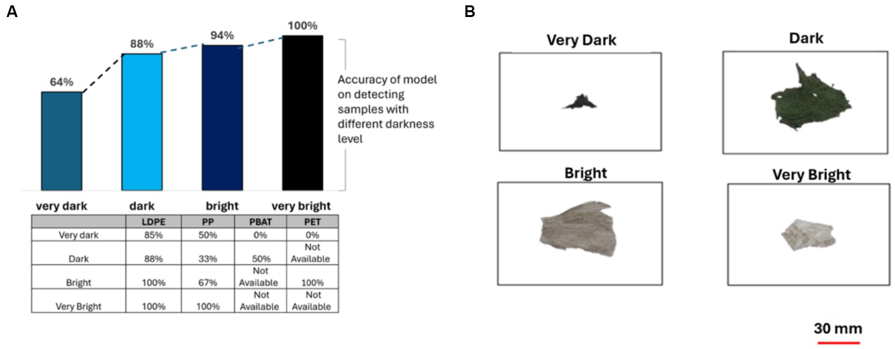
Figure 8. (A) The accuracy of PLS-DA classification model when categorizing based on darkness level, table shows results for different polymer classes; (B) samples from the composting plant representing four different plastic sizes (very dark, dark, bright and very bright).

When identifying brightly colored plastic samples, the accuracy was 100%. However, this rate dramatically decreased to 64% when identifying very dark colored plastics (see Figure 8). For LDPE, the model’s accuracy declined when identifying darker plastics. Nonetheless, its performance remained relatively high at 85% accuracy for detecting very dark plastics.

Likewise, for PBAT and PET, brighter plastics yielded better results. However, in the case of PP, dark plastics exhibited lower accuracy compared to very dark ones, primarily due to higher contamination levels, the presence of multicolor plastics, and the limited sample size, leading to potential bias.

The color of a plastic sample had an important impact on the accuracy of the model. The samples were allocated into four categories color: transparent, single color, multicolors and black. The single, transparent, multicolor and black plastic samples was 29, 12, 3, 3, respectively. When the plastic sample has a single color, the model achieves an impressively high accuracy of 83%. However, when the color of the plastic is transparent, the accuracy of the model slightly decreases to 75% due to the phenomenon of light transmission and scattering. For multicolor and black plastics, the accuracy of the model significantly drops to 33%, as illustrated in Figure 9. These findings highlight the crucial role that color plays in the performance of the model and emphasizes the need for further investigation and improvement in accurately predicting and categorizing plastic samples based on their colored properties.

Figure 9

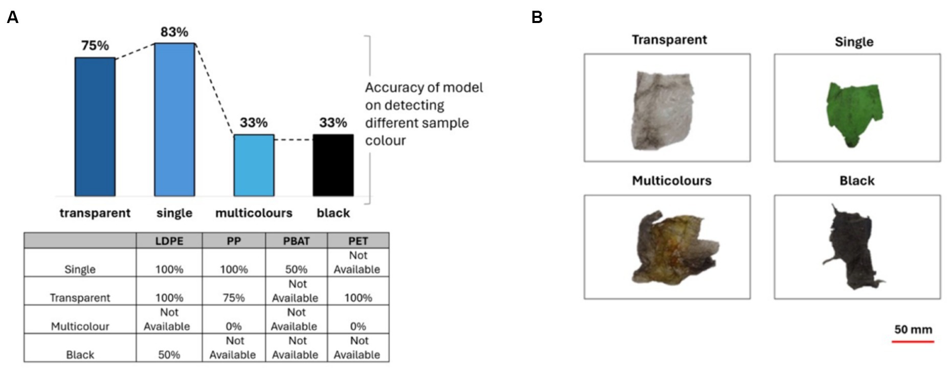
Figure 9. (A) The accuracy of PLS-DA classification model when categorizing plastics based on their colors, table shows results for different polymer classes; (B) showing representative images of samples representing transparent, single, multicolors and black plastics.

The model attained perfect accuracy in identifying single-color and transparent LDPE plastics but faced a decline to 50% accuracy for black LDPE. Regarding PP, while it achieved 100% accuracy for single-color plastics, the accuracy dropped to 75% for transparent ones, with a complete inability to detect multicolor plastics. For PBAT, the accuracy decreased to 50% for single-color PBAT, while achieving 100% accuracy for transparent PET.

The level of contamination of the samples was evaluated applying a level of contamination estimation algorithm. The plastic samples collected from the composting plant exhibited varying levels of contamination, with 4 samples categorized as low contamination, 20 samples classified as medium contamination, and 16 samples identified as high contamination. However, seven plastic samples could not have the contamination level determined due to a high darkness level, or similarities in sample color and contamination color.

The accuracy of identification was shown to be a function of the level of contamination. Specifically, the model achieved an accuracy of 100% when identifying plastics with low contamination, which subsequently decreased to 95 and 75% for samples with medium and high levels of contamination, respectively as shown Figure 10. For LDPE, the classification model achieved 100% accuracy across all categories. However, for PP and PBAT, the accuracy significantly decreased as the level of contamination increased.

Figure 10

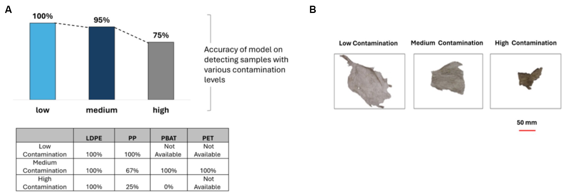
Figure 10. (A) The accuracy of PLS-DA classification model when categorizing plastics based on their level of contamination, table shows results for different polymer classes; (B) showing representative images of samples representing plastics with low contamination, medium contamination, and high contamination.

The size of plastic samples collecting from composting plant was measured using image processing method as explained in section 2.3.1.

Figure 11B illustrates the distribution of size of plastic sample collected from composting plant and images of samples from the composting plant representing four different plastic sizes (very small, small, medium and large). From Figure 11A, it was observed that the size has a modest impact on the accuracy of the classification model. The accuracy rate peaking at 92% for large pieces of plastic. However, as shown, the brightness level and color significantly affect the accuracy of the PLS-DA classification model. Therefore, only brightly colored and non-transparent plastic samples were selected to evaluate the effectiveness of the classification model. The result illustrates that the accuracy of model achieves 100% for all size categories (very small, small, medium and large) for plastics with a range of contamination when color and brightness are eliminated.

Figure 11

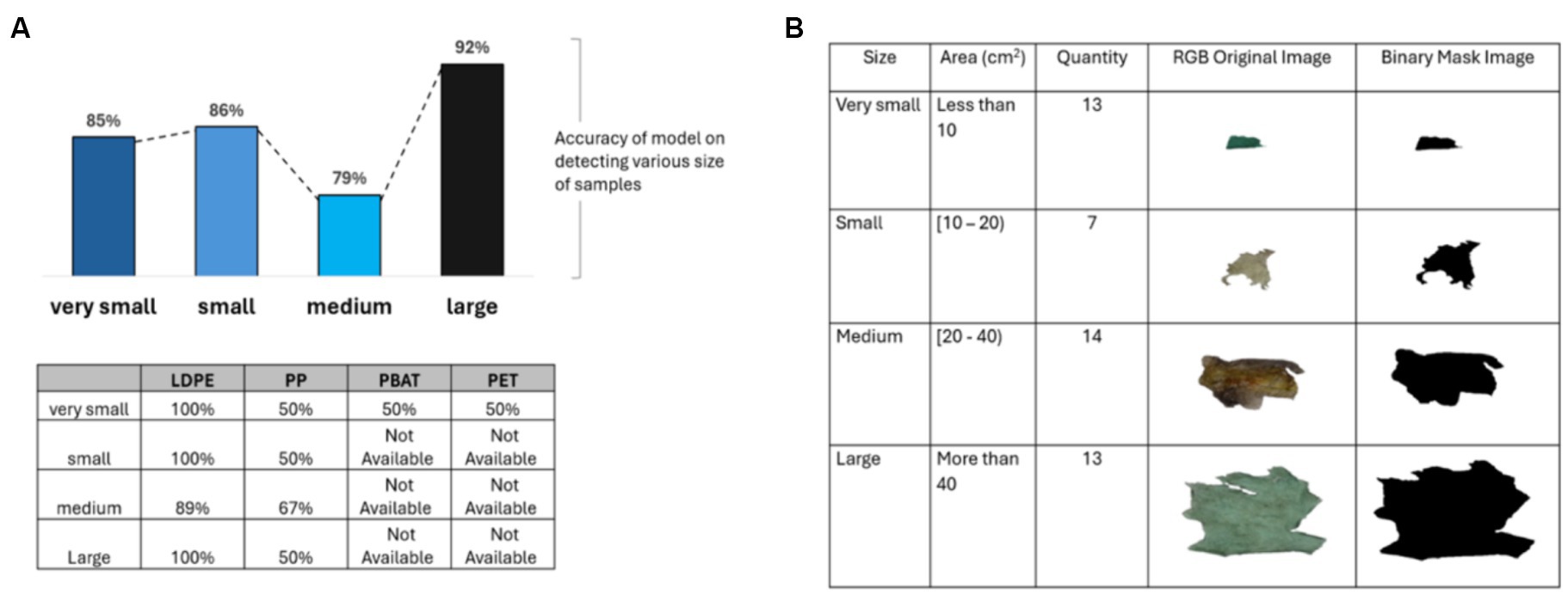
Figure 11. (A) The accuracy of PLS-DA classification model when categorizing plastics based on their size, table shows results for different polymer classes; (B) various size (very small, small, medium and large) of plastic samples from composting plant.

The model achieved 100% accuracy in identifying very small and small LDPE samples. However, the accuracy of the model on medium-sized LDPE samples experienced a dramatic decrease to 89%, mainly due to the predominant dark color of plastic samples in this category. Similarly, for PP and PBAT, the model would achieve 100% accuracy across all size categories if the samples were bright and not transparent. Accuracy dropped primarily due to the high darkness level of the samples rather than their size. For PET, due to its small size and transparency, the model only achieved a 50% accuracy rate (see Figure 11A).

Thickness was another features that was found to influence on the accuracy of the PLS-DA classification model. The information of field plastic samples thickness shows in Figure 12B. It classified into three categories which are thin, medium and thick.

Figure 12

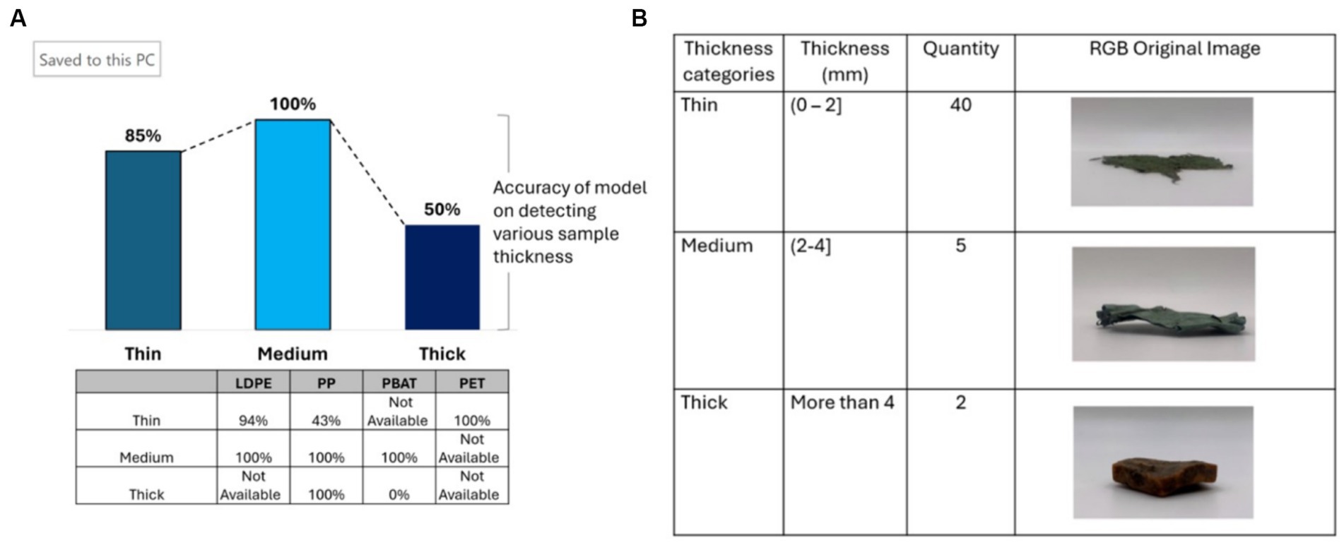
Figure 12. (A) The accuracy of PLS-DA classification model when categorizing plastic samples based on thickness, table shows results for different polymer classes; (B) the thickness of plastic samples from composting plant.

The model achieved peak accuracy of 100% when analyzing plastic thickness within the range of 2 mm to 4 mm. However, it’s important to note that this conclusion is based on a limited sample size, with only two thick plastic samples available for analysis, one of which was dark in color. When focusing solely on bright plastic samples, the model exhibited decreased accuracy in detecting thinner plastic due to the loss of spectral information. This finding is consistent with the observations made by Koinig et al. (2022) and Masoumi et al. (2012). For LDPE and PP, plastic within the range of 2 mm to 4 mm demonstrates the highest accuracy, reaching 100%. However, the model demonstrates significantly lower accuracy in detecting thin PP, achieving only 43%. In the case of thick plastic, PP achieves 100% accuracy, while PBAT attains 0%. This discrepancy can be attributed to the high darkness level of PBAT, which affects the spectral characteristics and compromises detection accuracy (see Figure 12A).

Seven plastic samples were selected from a composting plant with high brightness, uniform color and a range of contamination levels. These samples were subsequently reduced in size to large microplastic dimensions (<5 mm) (see Figure 13A). Identification of these plastic samples was carried out employing the PLS-DA model, which exhibited an accuracy of 100%.

Figure 13

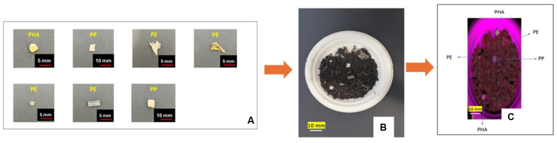
Figure 13. (A) Size and shape of large microplastic samples collected from composting plant; (B) optical image of large microplastic samples in end compost; (C) and hyperspectral image of the same sample color coded with the identification from the PLS-DA model.

To investigate the impact of being mixed into compost on the identification of these large microplastic samples, we mixed them with compost obtained from the IC plant. Using the PLS-DA model this mixed sample was tested, and the accuracy remained consistently high at 80% as long as all the samples were visible within the compost, as shown in Figures 13B,C.

4 Discussion

Compostable plastics have witnessed a surge in popularity as a potential substitute for conventional (non-compostable) plastics. However, to fully realize the benefits of compostable plastics, it is crucial that they are prevented from entering the environment, including soil and marine ecosystems. In the current waste management system, compost often contains contaminants, which significantly reduces the quality of the compost (Edo et al., 2022). Density sorting and trommel techniques are currently used to eliminate contaminants, but they are not able to remove all microplastics in compost. To help address this problem, we have investigated the use of SWIR-HSI together with PLS-DA model detect plastic and large microplastic content from real world IC systems.

Our experiments have shown that PLS-DA model can accurately detect a wide range of conventional (non-compostable) plastics that are typically found to contaminate compost during IC processing including PET, PP, and PE. We trained our model first on virgin plastics and soil contaminated plastic but then tested the model on plastic collected from an IC plant. These plastic fragments were of various sizes (The average size is 27.14 cm²), colors, thickness and brightness. Crucially they were also contaminated with earth and compost that was ingrained into the fabric of the plastic as a result of being of through the IC process. Nevertheless, our model was able to identify them to 80% of accuracy.

In this study, we compared three different spectral pre-processing methods (SNV + MC, SG + MC, and SG + SNV + MC) to improve multivariate classification model, and exploratory analysis. Our results show that SG + SNV + MC yielded the best classification results. The combination of SNV and SG is better than utilizing SNV and SG alone because it can leverage the strengths of both methods. SNV corrects for multiplicative effects while SG further enhances the data by reducing noise and revealing underlying information.

When applying our PLS-DA classification model to field plastic samples collected from the IC plant we were interested in understanding which aspect of their condition would affect the accuracy of their identification. We focused on various parameters we could measure using image processing techniques: darkness, size, color, and contamination level. The darkness level had a significant impact on the accuracy of the classification model. Brightly-colored plastics had a lower misclassification rate compared to dark-colored plastics. This is because opaque plastics absorb most of the radiation in the SWIR region, making it difficult for spectroscopic analysis to penetrate the material and detect its chemical composition. The absorption of radiation by dark-colored plastics resulted in a low signal-to-noise ratio, making it challenging to distinguish them from other materials in the sample (Rani et al., 2019).

The color of a plastic sample also had a profound impact on the accuracy of the model. The results showed that the accuracy decreased moderately to 75% when identifying transparent plastics and dramatically dropped to 33% when identifying black and multicolored plastics. In contrast size did not affect accuracy greatly once the other factors of darkness, color and sample contamination were removed.

Our PLS-DA classification model is capable of detecting large microplastics in the compost and correctly identifying them. In addition to darkness, color and size, the level of contamination is an important parameter that affected the accuracy of the model. The identification of plastic samples with a high level of contamination proves to be challenging for the PLS-DA model. The reason for this is that the model identifies the samples in a pixel-by-pixel fashion and then makes an overall determination according to the classification model. When large number of pixels are misidentified due to contamination this confuses the model and we currently do not have a method to recognize this is occurs and eliminate these pixels from the classification algorithm. The thickness of the plastic is another critical factor that significantly impacts the model. Thinner plastic tends to provide inadequate spectral information.

The success of our approach invites consideration as to how our technique can be employed to help the waste processing sector. Clearly, we have shown that identifying compostable plastics such as PLA, PBAT, and PHA from a mixed recycling stream is possible, even when there is moderate contamination. It is noteworthy that PET and PLA can be easily distinguished from each other which is a problem for traditional IR detection systems. There is a high commercial value of increasing the purity PET recycling streams what might justify the expenditure of investment of a SWIR-HSI system. The PLA that is identified could also be separated and sent to an industrial composter.

Industrial composting plants could benefit from deploying a SWIR-HSI together with PLS-DA model to help them decrease contamination of the end compost and thus increase its value both commercially and environmentally. Because it can give real time information it could quantify large microplastics content as a function of process variables thus helping operators to optimize their system to minimize them. By identifying the large plastic fragments separated by the trommel, the PLS-DA model could also identify any compostable plastics are failing to biodegrade and feed this information back to the manufacturers.

Anaerobic digestion (AD) plants could also use this method to assess in real time the plastics coming into their systems mixed in with food and agricultural waste. At the moment it is standard practice to remove all plastics whether they are compatible with AD plants or not. Combining SWIR-HSI with PLS-DA model could help AD plants identify and separate compostable plastics and send them to an IC plant. Similarly, this approach could be used to assess the microplastic content of the digestate and to determine the mix of plastics in it.

5 Conclusion

We have showed that hyperspectral imaging technology with our developed classification model can detect and identify plastics and large microplastics obtained from industrial composters.

Our model demonstrated an overall detection rate of 90.3% when detecting microplastic within testing dataset and 80% of large microplastics contaminated with soil in compost sample obtained from an industrial composting plant. In comparison to the earlier study conducted by Serranti et al., our model exhibited superior performance specifically in recognizing Polyethylene (PE). Additionally, our model exhibited improved performance in detecting dark large microplastic low-density polyethylene (LDPE) compared to previous work, achieving an 85% accuracy, whereas the model of Zhao et al. achieved 58%. Both studies underscored the challenge of accurately identifying dark large microplastics. The SIMCA model developed by Vidal et al. shows excellent accuracy of 99% of detecting microplastics in sand. Their better accuracy might be due to the lower organic content in sand compared with compost. It is noteworthy that both studies highlighted the limitation of size on the accuracy of microplastic detection using SIMCA and PLSDA classification model.

Regarding the plastic features influencing the model’s accuracy, our findings indicated that characteristics such as darkness, size, thickness, color, and level of contamination significantly impact the performance of the model. These results are consistent with the conclusions drawn in studies conducted by Masoumi et al. (2012) and Shan et al. (2019). Specifically, darker color, smaller size, thinner and a high level of contamination were identified as factors contributing to lower accuracy in the classification model. This alignment with previous research reinforces the importance of considering these specific plastic attributes when developing and assessing detection models for optimal performance (Shan et al., 2019; Faltynkova et al., 2021).

Furthermore, the breadth of materials that our model successfully identified surpassed the range covered in previous research. Our model’s ability to identify a broader spectrum of large microplastic materials showcases its enhanced capabilities and expands the scientific understanding of microplastic pollution.

Besides, the identification results from both SWIR-HSI and FTIR indicated the presence of compostable plastic (PBAT) in the batch collected from the composting plant. This suggests that the composting process may not be fully optimized to handle such materials. Several factors, such as the short duration of the In-Vessel Composting (IVC) process, a low carbon-to-nitrogen ratio, and the thickness of compostable plastic, could contribute to the failure of effectively composting compostable plastics (Ruggero et al., 2020). Addressing these factors is essential for enhancing the composting efficiency of such materials in the composting plant. This results aligns with the Porterfield et al.’s findings (Porterfield et al., 2023).

However, the limitation of this study is that the threshold for image segmentation determined the resolution thus, the smallest plastic sample we could detect was 2 mm. Nevertheless, the findings highlight the substantial progress made by our model in accurately detecting microplastics and the potential it holds for further research and practical applications in waste processing plants.

Data availability statement

The raw data supporting the conclusions of this article will be made available by the authors, without undue reservation.

Author contributions

NT: Data curation, Methodology, Writing – review & editing, Formal analysis, Investigation, Software, Validation, Visualization, Writing – original draft. HH: Formal analysis, Funding acquisition, Project administration, Resources, Supervision, Writing – review & editing. MM: Funding acquisition, Project administration, Resources, Supervision, Writing – review & editing, Conceptualization, Data curation, Methodology.

Funding

The author(s) declare that financial support was received for the research, authorship, and/or publication of this article. The research was funded through UKRI grants NE/V010735/1, EP/Y003993/1, EP/S024883/1.

Acknowledgments

We thank Sophia Tazi for her help with this work.

Conflict of interest

The authors declare that the research was conducted in the absence of any commercial or financial relationships that could be construed as a potential conflict of interest.

Publisher’s note

All claims expressed in this article are solely those of the authors and do not necessarily represent those of their affiliated organizations, or those of the publisher, the editors and the reviewers. Any product that may be evaluated in this article, or claim that may be made by its manufacturer, is not guaranteed or endorsed by the publisher.

References

Amigo, J. M., Babamoradi, H., and Elcoroaristizabal, S. (2015). Hyperspectral image analysis. A tutorial. Anal. Chim. Acta 896, 34–51.

Google Scholar

Bonifazi, G., D'agostini, M., Dall'ava, A., Serranti, S., and Turioni, F. (2013). “A new hyperspectral imaging based device for quality control in plastic recycling” Prague, Czech Republic: Optical Sensors (2013), 365–377.

Google Scholar

Chaczko, Z., Wajs-Chaczko, P., Tien, D., and Haidar, Y. Detection of microplastics using machine learning. In: 2019 International Conference on Machine Learning and Cybernetics (ICMLC) (2019). Kobe, Japan: IEEE, 1–8.

Google Scholar

Corcoran, P. L. (2022). “Degradation of microplastics in the environment” in Handbook of microplastics in the environment (Switzerland: Springer).

Google Scholar

Cucuzza, P., Serranti, S., Bonifazi, G., and Capobianco, G. (2021). Effective recycling solutions for the production of high-quality pet flakes based on hyperspectral imaging and variable selection. J. Imaging 7:181. doi: 10.3390/jimaging7090181

PubMed Abstract | Crossref Full Text | Google Scholar

De Souza Machado, A. A., Lau, C. W., Kloas, W., Bergmann, J., Bachelier, J. B., Faltin, E., et al. (2019). Microplastics can change soil properties and affect plant performance. Environ. Sci. Technol. 53, 6044–6052. doi: 10.1021/acs.est.9b01339

PubMed Abstract | Crossref Full Text | Google Scholar

Edo, C., Fernández-Piñas, F., and Rosal, R. (2022). Microplastics identification and quantification in the composted organic fraction of municipal solid waste. Sci. Total Environ. 813:151902. doi: 10.1016/j.scitotenv.2021.151902

PubMed Abstract | Crossref Full Text | Google Scholar

EEA (2020). Biodegradable and compostable plastics — challenges and opportunities [Online]. Available at: https://www.eea.europa.eu/publications/biodegradable-and-compostable-plastics (Accessed June 5, 2021).

Google Scholar

Faltynkova, A., Johnsen, G., and Wagner, M. (2021). Hyperspectral imaging as an emerging tool to analyze microplastics: a systematic review and recommendations for future development. Microplast. Nanoplast. 1, 1–19,

Google Scholar

Hoo, Z. H., Candlish, J., and Teare, D. (2017). What is an roc curve? Emerg. Med. J. 34, 357–359. doi: 10.1136/emermed-2017-206735

Crossref Full Text | Google Scholar

Hu, J., He, D., Zhang, X., Li, X., Chen, Y., Wei, G., et al. (2022). National-scale distribution of micro (meso) plastics in farmland soils across China: implications for environmental impacts. J. Hazard. Mater. 424:127283. doi: 10.1016/j.jhazmat.2021.127283

PubMed Abstract | Crossref Full Text | Google Scholar

Hyspex (2019). Quick Reference Guide HySpex Ground v4.9.

Google Scholar

ISO2020. (2020). Iso definitions of key terms for plastic pollution [Online]. Available at: https://www.iso.org/files/live/sites/isoorg/files/store/en/Pub100472.pdf (Accessed March 7, 2024).

Google Scholar

Jolliffe, I. (2005). “Principal component analysis” in Encyclopedia of statistics in behavioral science.

Google Scholar

Karlsson, T. M., Grahn, H., Van Bavel, B., and Geladi, P. (2016). Hyperspectral imaging and data analysis for detecting and determining plastic contamination in seawater filtrates. J. Near Infrared Spectrosc. 24, 141–149. doi: 10.1255/jnirs.1212

Crossref Full Text | Google Scholar

Koinig, G., Friedrich, K., Rutrecht, B., Oreski, G., Barretta, C., and Vollprecht, D. (2022). Influence of reflective materials, emitter intensity and foil thickness on the variability of near-infrared spectra of 2D plastic packaging materials. Waste Manag. 144, 543–551. doi: 10.1016/j.wasman.2021.12.019

PubMed Abstract | Crossref Full Text | Google Scholar

Kumar, A. (2022). Machine Learning – Sensitivity vs Specificity Difference [Online]. Available at: https://vitalflux.com/ml-metrics-sensitivity-vs-specificity-difference/ (Accessed February 1, 2023).

Google Scholar

Manu, M., Luo, L., Kumar, R., Johnravindar, D., Li, D., Varjani, S., et al. (2023). A review on mechanistic understanding of microplastic pollution on the performance of anaerobic digestion. Environ. Pollut. 325:121426. doi: 10.1016/j.envpol.2023.121426

Crossref Full Text | Google Scholar

Masoumi, H., Safavi, S. M., and Khani, Z. (2012). Identification and classification of plastic resins using near infrared reflectance. Int. J. Mech. Ind. Eng. 6, 213–220,

Google Scholar

Neves, M. D. G., Poppi, R. J., and Breitkreitz, M. C. (2022). Authentication of plant-based protein powders and classification of adulterants as whey, soy protein, and wheat using Ft-Nir in tandem with Oc-Pls and Pls-Da models. Food Control 132:108489. doi: 10.1016/j.foodcont.2021.108489

Crossref Full Text | Google Scholar

OpenCV (2023). Image Thresholding [Online]. Available at: https://docs.opencv.org/4.x/d7/d4d/tutorial_py_thresholding.html (Accessed October 10, 2023).

Google Scholar

PAS100 (2022). Guidance on assessing Pas 100 test results against Sepa plastic limits [Online]. Available at: https://www.qualitycompost.org.uk/upload/files/f68_Guidance_on_assessing_Pas_100_test_results_against_Sepa_plastic_limits_September_2022_final.pdf (Accessed October 10, 2023).

Google Scholar

Porterfield, K. K., Hobson, S. A., Neher, D. A., Niles, M. T., and Roy, E. D. (2023). Microplastics in composts, digestates, and food wastes: a review. J. Environ. Qual. 52, 225–240. doi: 10.1002/jeq2.20450

PubMed Abstract | Crossref Full Text | Google Scholar

Rani, M., Marchesi, C., Federici, S., Rovelli, G., Alessandri, I., Vassalini, I., et al. (2019). Miniaturized near-infrared (Micronir) spectrometer in plastic waste sorting. Materials 12:2740. doi: 10.3390/ma12172740

Crossref Full Text | Google Scholar

Rinnan, Å., Van Den Berg, F., and Engelsen, S. B. (2009). Review of the most common pre-processing techniques for near-infrared spectra. TrAC Trends Anal. Chem. 28, 1201–1222. doi: 10.1016/j.trac.2009.07.007

Crossref Full Text | Google Scholar

Ruggero, F., Carretti, E., Gori, R., Lotti, T., and Lubello, C. (2020). Monitoring of degradation of starch-based biopolymer film under different composting conditions, using TGA, FTIR and SEM analysis. Chemosphere 246:125770:10.1016/j.chemosphere.2019.125770,

Google Scholar

Serranti, S., Fiore, L., Bonifazi, G., Takeshima, A., Takeuchi, H., and Kashiwada, S. (2019). “Microplastics characterization by hyperspectral imaging in the SWIR range” in SPIE future sensing technologies (Tokyo, Japan: International Society for Optics and Photonics), 1119710.

Google Scholar

Serranti, S., Palmieri, R., Bonifazi, G., and Cózar, A. (2018). Characterization of microplastic litter from oceans by an innovative approach based on hyperspectral imaging. Waste Manag. 76, 117–125. doi: 10.1016/j.wasman.2018.03.003

PubMed Abstract | Crossref Full Text | Google Scholar

Shan, J., Zhao, J., Zhang, Y., Liu, L., Wu, F., and Wang, X. (2019). Simple and rapid detection of microplastics in seawater using hyperspectral imaging technology. Anal. Chim. Acta 1050, 161–168. doi: 10.1016/j.aca.2018.11.008

PubMed Abstract | Crossref Full Text | Google Scholar

Taneepanichskul, N., Hailes, H. C., and Miodownik, M. (2023). Automatic identification and classification of compostable and biodegradable plastics using hyperspectral imaging. Front. Sustain. 4:1125954. doi: 10.3389/frsus.2023.1125954

Crossref Full Text | Google Scholar

Taneepanichskul, N., Purkiss, D., and Miodownik, M. (2022). A review of sorting and separating technologies suitable for compostable and biodegradable plastic packaging. Front. Sustain. 3:901885. doi: 10.3389/frsus.2022.901885

Crossref Full Text | Google Scholar

Tian, W., Song, P., Zhang, H., Duan, X., Wei, Y., Wang, H., et al. (2022). Microplastic materials in the environment: problem and strategical solutions. Prog. Mater. Sci. 132:101035. doi: 10.1016/j.pmatsci.2022.101035

Crossref Full Text | Google Scholar

Tong, H., Zhong, X., Duan, Z., Yi, X., Cheng, F., Xu, W., et al. (2022). Micro-and nanoplastics released from biodegradable and conventional plastics during degradation: formation, aging factors, and toxicity. Sci. Total Environ. 833:155275. doi: 10.1016/j.scitotenv.2022.155275

PubMed Abstract | Crossref Full Text | Google Scholar

Vidal, C., and Pasquini, C. (2021). A comprehensive and fast microplastics identification based on near-infrared hyperspectral imaging (Hsi-Nir) and chemometrics. Environ. Pollut. 285:117251. doi: 10.1016/j.envpol.2021.117251

PubMed Abstract | Crossref Full Text | Google Scholar

Vithanage, M., Ramanayaka, S., Hasinthara, S., and Navaratne, A. (2021). Compost as a carrier for microplastics and plastic-bound toxic metals into agroecosystems. Curr. Opin. Environ. Sci. Health 24:100297. doi: 10.1016/j.coesh.2021.100297

Crossref Full Text | Google Scholar

Wold, S., Sjöström, M., and Eriksson, L. (2001). Pls-regression: a basic tool of chemometrics. Chemom. Intell. Lab. Syst. 58, 109–130. doi: 10.1016/S0169-7439(01)00155-1

Crossref Full Text | Google Scholar

Xiong, Z., Sun, D.-W., Zeng, X.-A., and Xie, A. (2014). Recent developments of hyperspectral imaging systems and their applications in detecting quality attributes of red meats: a review. J. Food Eng. 132, 1–13. doi: 10.1016/j.jfoodeng.2014.02.004

Crossref Full Text | Google Scholar

Xu, J.-L., Thomas, K. V., Luo, Z., and Gowen, A. A. (2019). FTIR and Raman imaging for microplastics analysis: state of the art, challenges and prospects. TrAC Trends Anal. Chem. 119:115629. doi: 10.1016/j.trac.2019.115629

Crossref Full Text | Google Scholar

Zhang, Y., Wang, X., Shan, J., Zhao, J., Zhang, W., Liu, L., et al. (2019). Hyperspectral imaging based method for rapid detection of microplastics in the intestinal tracts of fish. Environ. Sci. Technol. 53, 5151–5158. doi: 10.1021/acs.est.8b07321

PubMed Abstract | Crossref Full Text | Google Scholar

Zhao, J., Liu, L., Zhang, Y., Wang, X., and Wu, F. (2018). A novel way to rapidly monitor microplastics in soil by hyperspectral imaging technology and chemometrics. Environ. Pollut. 238, 121–129. doi: 10.1016/j.envpol.2018.03.026

Crossref Full Text | Google Scholar