Beneficial use of sediments to restore a Chesapeake Bay marsh island

1 Introduction

Rising seas, shoreline erosion, extreme weather and flooding events (Sweet et al., 2019; NOAA, 2023) combined with accelerating loss of biodiversity (IPBES, 2019) are driving interest in the use of natural infrastructure (NI). In coastal regions, NI (also commonly referred to as Nature Based Solutions, NBS) involve the strategic use of natural ecosystems, like marshes, islands, seagrass beds and oyster reefs, either alone or in combination with conventional hardened infrastructure (e.g., bulkheads and breakwaters.), to provide engineering (e.g., storm risk reduction, erosion control) and environmental benefits for both humans and wildlife. NI can reduce erosion and flood risks to communities (Spalding et al., 2014; Chausson et al., 2020), provide recreational opportunities (Winter et al., 2019) and improve human health and well-being (Williams, 2017), while providing habitat for vulnerable wildlife like migratory birds and a variety of aquatic organisms (Unguendoli et al., 2023).

Concurrent with the growing interest in NI, the use of dredged sediments for coastal habitat restoration (often referred to as Beneficial Use) is also gaining traction. Sediment is a critical resource for vegetated estuarine and coastal habitats. Delivery of sediments during flood tides is one of the primary processes by which these habitats build elevation, and is critical to their ability to keep pace with rising sea levels (Morris et al., 2002). Sediments that are removed from navigation channels through dredging have traditionally been placed in upland containment cells or disposed of in the open ocean (Zentar et al., 2009). Both of these fates result in a net removal of sediment from coastal systems, which contributes to the vulnerability of salt marshes, seagrass beds, and coastal forests to rising sea level. In recent years, traditional sediment disposal methods have become increasingly cost-prohibitive and in some cases, contrary to individual state requirements [Code of Maryland Regulations (COMAR), 1994]. Combining habitat restoration with navigation dredging is increasingly being viewed as a win-win for maintaining navigable waterways and ecosystem sustainability in the face of sea level rise (SLR) and extreme events (Bridges et al., 2014; Raposa et al., 2020).

Despite the advantages of NI approaches for enhancing coastal resilience, widespread acceptance and use of NI remains elusive, in part due to the inherent uncertainties associated with the performance of natural ecosystems (Nelson et al., 2020). Hardened infrastructure like seawalls, revetments, and bulkheads are static features designed to withstand specific wave heights, runup, and overtopping events (Sterr, 2008; Rosenzweig et al., 2011). Natural infrastructure like islands, marshes, and oyster reefs are also capable of withstanding such forces but our understanding of how much force a given NI can withstand is limited. Further, because NI are living features, they actively adapt to changing environmental conditions like SLR, droughts, and storms (Rodriguez et al., 2014; Sutton-Grier et al., 2015). The ability of NI to adapt makes it challenging not only to predict how much wave energy a given feature can endure, but also how that threshold might change in the future as a site matures. In contrast, the static nature of hardened infrastructure, availability of engineering and design criteria to guide their implementation, and historical reliance on hardened features continues to make them the default choice for coastal protection in most situations. Increased acceptance and widespread use of NI approaches requires data-driven analysis of NI project performance (Davis et al., 2021). Currently, published monitoring data are available for a handful of projects across the U.S. for which dredged sediments were used for restoration of coastal habitats (McAtee et al., 2020; Douglas et al., 2021; Davis et al., 2022; Puchkoff and Lawrence, 2022; Raposa et al., 2022). While the practice of using dredged sediments to create coastal habitats is not new (dredge material-created islands are a common feature along many navigation channels), most historical projects were implemented with the primary goal of convenient disposal of dredged sediments rather than creation of specific habitats. As a result, the data required to support performance analysis of historical projects is exceedingly rare.

In the current contribution we attempt to help fill the knowledge gap surrounding the performance of coastal NI created from dredged sediments by providing a synthesis of the early monitoring data from Swan Island, MD. Swan Island, which functions as a natural wave break for the nearby town of Ewell on adjacent Smith Island, suffered from rapid rates of erosion, habitat fragmentation, and subsidence in recent decades. In 2019, to address these challenges, the US Army Corps of Engineers (USACE) Baltimore District placed ~60,000 cubic yards (45,873 cubic meters) of sediment on 12 acres (4.8 hectares) of Swan Island. The goals of this project included increasing the elevation capital of Swan Island to maximize its function as a wave break, enhancing the diversity of habitats on the island, and increasing resilience to future sea level rise. The data provided here describe changes in island topography, vegetative communities, and soil properties over three full calendar years post construction and highlight both the successes and shortcomings of the implemented project design. This analysis provides insight into the challenges with, and benefits of, restoring coastal marsh islands with dredged sediments.

2 Materials and methods

2.1 Restoration activities

Swan Island, Maryland is a 25-acre island located at the southern extent of the Martin National Wildlife Refuge, adjacent to a federal navigation channel in Chesapeake Bay (Figure 1). Previous losses of marsh island habitat in the mid-Chesapeake Bay due to relative sea level rise and erosion are well-documented (Erwin et al., 2011, Marbán et al., 2019). Like other islands in the region, Swan had experienced significant shoreline erosion in recent decades (Perini Management Services, 2014) and the interior marsh was highly fragmented. The apparent vulnerability of Swan Island to further losses made it a prime candidate for restoration. The sediments used for restoration were generated from routine maintenance dredging of multiple reaches of the navigation channel that provides access to the town of Ewell. The sediments used to restore Swan Island were transported up to 2 km. Prior to sediment placement, the project area consisted predominantly of highly fragmented low marsh vegetated by Spartina alterniflora. The placement design involved grading the placed sediments to produce a smooth transition of elevations that support low marsh, high marsh, and dune vegetation. The target elevations for regions of the island slated to become low marsh, high marsh and dune were 0.28, 0.59 and > 0.5 to 1.01 m NAVD88, respectively based on the elevation distribution of these habitats in the local area. The design included the use of sandier sediments to build dunes and high marsh, while the finer material was reserved for the low marsh. As part of the restoration effort, a shore-parallel sill of stacked 61 cm concrete armoring units (A-Jack^®, Contech; West Chester, OH) was installed along the northeast shoreline (Figure 1). The structure was pyramidal (2 blocks wide on the bottom, one block on top) and designed to extend to +0.61 m MLLW.

Figure 1

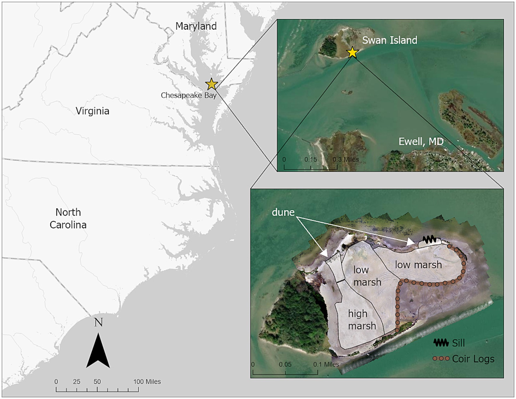
Figure 1. Project location. Swan Island location within Chesapeake Bay (top), Swan Island position relative to the town of Ewell, MD (middle), placement of coir log containment barrier, sill, and planned distribution of habitats. Map images are the intellectual property of Esri and are used under license.

The project was designed to avoid impacts to adjacent subtidal habitats, including submerged aquatic vegetation (SAV). Prior to dredge material placement, a containment structure consisting of coir logs (two logs stacked vertically) held in place with wooden stakes was constructed along the north and western edge of the subtidal bight on the southeast portion of the island (Figure 1). The goal of this structure was to restrict the placed sediments from spreading into the bight which was vegetated with Ruppia maritima, the dominant SAV species in the region.

Maintenance dredging of the Big Thorofare (the channel directly adjacent to the southern shoreline of Swan Island) occurred between November 2018 and March 2019. Material was placed via a hydraulic pipeline dredge and then contoured with a low-pressure excavator. Dredging and material placement were restricted to October through March in order to avoid impacts to adjacent SAV habitat and other living resources. Upon completion of dredging and grading activities (April 2019), the project area was planted with either Spartina patens (all areas above 0.28 m NAVD88) or S. alterniflora (all areas below 0.28 m). Planting was conducted by hand in a grid design with 0.45 m (S. patens) or 0.61 m (S. alterniflora) spacing among individual plugs. In total, 200,000 5 cm nursery-grown plugs were planted.

2.2 On-the-ground sampling

Field data collection efforts involved characterization of vegetative communities, sediments, porewater sulfide and nutrient concentrations, island surface topography, and changes in those parameters over time. Most of these characteristics were documented once before sediment placement (2018) and then annually at fixed locations after sediment placement and initial planting was completed (2019–2022). Specific parameters varied somewhat among years (Table 1).

Table 1

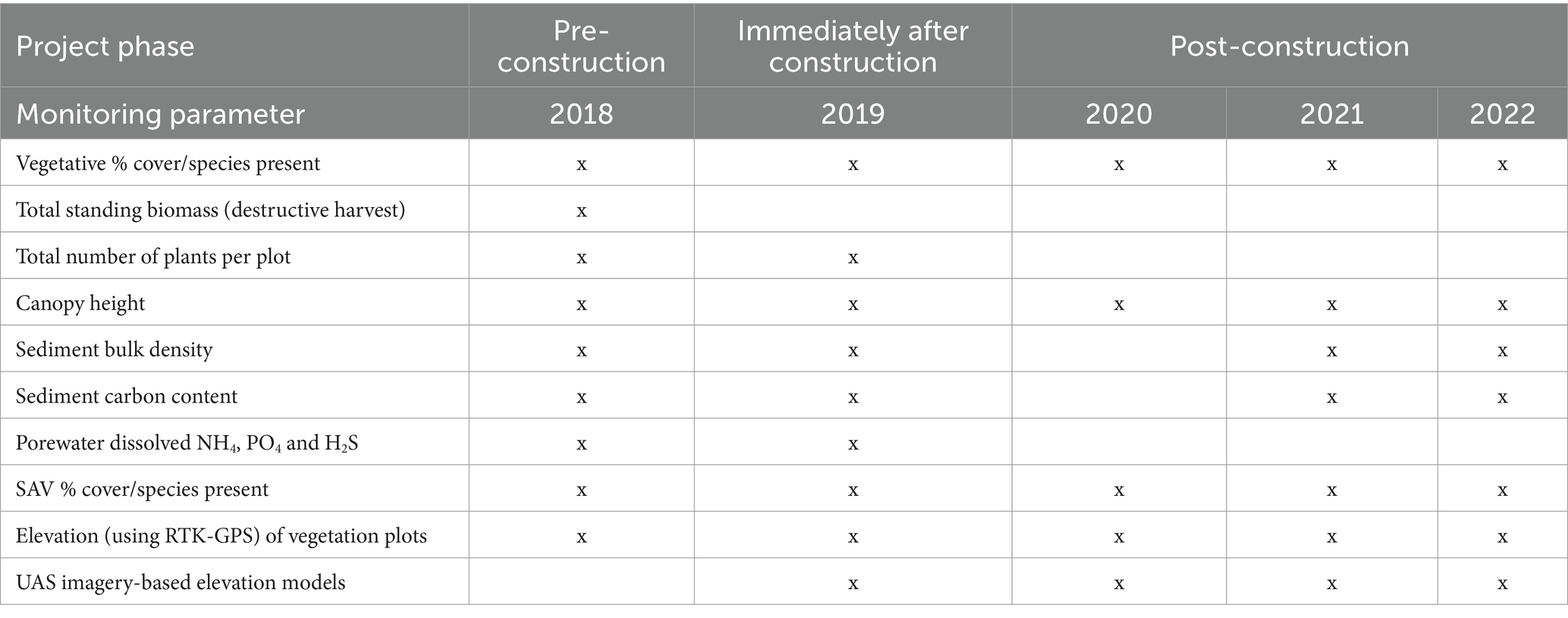
Table 1. Sampling parameters and project phase/year in which each was collected.

2.2.1 Pre-placement (2018)

Sampling to establish pre-placement conditions was conducted in August 2018. The goal was to understand the distribution of existing vegetation with respect to elevation and to document edaphic conditions in the native marsh platform. The full elevation range occupied by S. alterniflora (the dominant species present) was established using RTK (Real-Time Kinematic)-GNSS techniques (hereafter referred to as GPS). A temporary bench mark which consisted of a 2 m stainless steel rod driven into the berm along the island’s southern shoreline was established to support GPS data collections. Simultaneous static GPS data collections were made on the temporary benchmark and a geodetic survey mark located at the Tawes Museum (PID: DH7949) in Crisfield, MD. The temporary mark’s position and orthometric height were determined through post-processing using Trimble Business Center (TBC) and tied to the National Spatial Reference System (NSRS) using the Online Positioning User Service (OPUS). A second GPS rover receiver was attached to a modified bicycle and programmed to collect data in 5 s-continuous topo mode while the bicycle was rolled across the island surface. Additional point collections were made with the rover attached to a 2 m fixed height pole. Field data were collected and stored in the Trimble handheld controller and then exported to Trimble Business Center for review and quality checks, then subsequently exported to ArcGIS Pro v3.1.3 (Esri Inc., Redlands, CA, United States) as shapefiles.

The elevation range occupied by S. alterniflora was divided into 10 cm “bins” and three vegetation sampling plots (1 m²) were established at haphazardly selected locations within each bin. At each plot, total percent cover by species was estimated according to the North Carolina Vegetation survey approach (Peet et al., 1998). One quarter of each plot was destructively harvested for analysis of total standing biomass by clipping all vegetation with scissors at the sediment surface. Clipped vegetation was stored at 4^o C until processing (within 1 week). Processing of clipped biomass involved separating S. alterniflora into live and dead fractions. Each fraction was rinsed to remove sediment before drying at 60°C for 48 h, then weighed to determine total live standing biomass.

A single sediment core (3 cm diameter by 10 cm deep) was collected from each vegetation sampling plot. The entire content of each core was extruded, then dried at 60°C for 72 h and weighed for analysis of dry bulk density. Dried cores were then ground with a mechanical ball mill (Retsch, mixer mill 400) and subsampled for analysis of carbon content with a Costech ECS 4010 Elemental Analyzer. A single porewater sample (10 cm deep) was collected from each plot using a push-point sampler and peristaltic pump with gas tight tubing and filtered (0.45 μm nylon filters) immediately upon collection. Subsamples for analysis of hydrogen sulfide (H₂S) were filtered into zinc acetate, and refrigerated until analysis with Cline’s method (Cline, 1968). Porewater subsamples for ammonium (NH₄⁺) and orthophosphate (PO₄³⁻) were stored frozen until analysis by standard spectrophotometric methods (Parsons et al., 1984). Sediment and porewater samples were restricted to 10 cm in depth to capture conditions in the active root zone.

A slightly modified version of the standard protocols employed by the Maryland Department of Natural Resources’ Living Resource Assessment group (Burdick and Kendrick, 2001; Landry and Golden, 2018) were used to document SAV within the subtidal bight on the southeastern corner of the island that was separated from the intended placement area by coir logs (Figure 1, bottom). Briefly, two transects were established, one in each “lobe” of the bight by stretching a transect tape across the full length of the SAV bed. Ten fixed monitoring plots (0.25 m² quadrats) were distributed at equal distances (full length of transect/10) across each transect. Total percent cover of SAV within each plot was estimated visually and the length of 5 randomly selected shoots were recorded. Relative water depth was also recorded for each plot. Orthometric elevation was determined by RTK-GPS at 5 m intervals along the full length of each transect.

2.2.2 Post-placement (2019–2022)

2.2.2.1 Vegetation and sediments

The post-placement survey strategy was designed to track changes in each of the created habitats (Dune, High Marsh, Low Marsh) over time. A series of permanent vegetation monitoring transects were established using a stratified random sampling approach to capture the full range of elevations and vegetative species present within each created habitat type. All transects extended the full length of the created habitat or 100 m, whichever was greater. Five long-term monitoring plots were established at equal distances along each transect. In all, 90 fixed monitoring plots were established (Figure 2).

Figure 2

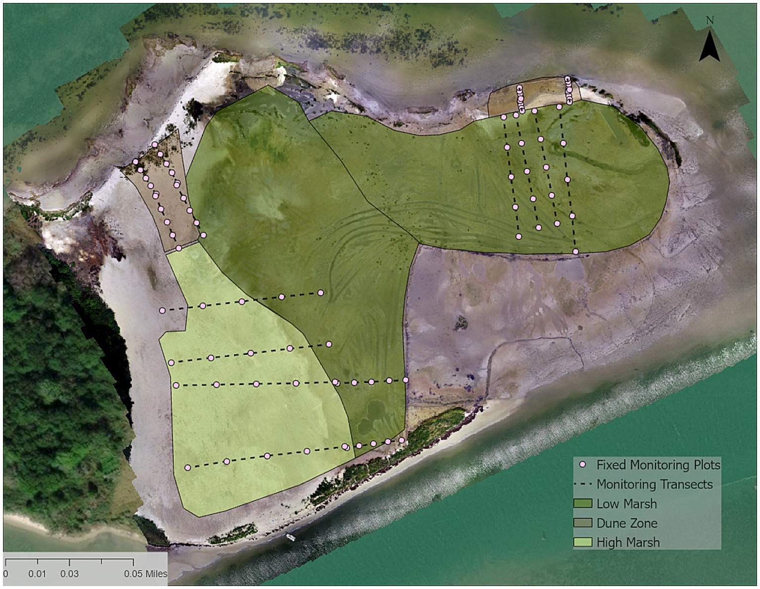
Figure 2. Plot-based sampling scheme. Fixed monitoring plots were evenly distributed along transects in each of the created habitat types. Map image is the intellectual property of Esri and is used under license.

Plot-based monitoring involved documentation of the species present, counting the total number of planting units (2019) or estimating total percent cover by species (2020–2022), measuring the height of the 5 tallest stems, and documenting sediment surface elevation at the approximate center of each plot with GPS. We arbitrarily chose one transect from each zone for collection of sediment and porewater samples from all monitoring plots along the transect. Sediment sampling involved collection of a sediment core (3.5 cm diameter by 10 cm deep) for analysis of bulk density and organic carbon content, and porewater samples were collected from 10 cm depth for analysis of H₂S, NH₄⁺, and PO₄³⁻ using the methods described previously, in 2019 only. Sediment cores were collected in 2019, 2021, and 2022.

SAV monitoring involved documentation of the species present, estimating total SAV percent cover, individual species cover, and measuring canopy height/shoot length and relative water depths within 0.25 m² quadrats along transects similar to those established pre-placement.

2.2.2.2 Positional data

Post-placement elevation surveys were conducted in 2019, 2021, and 2022, with a Real-Time Kinematic (RTK) surveying technique that involved the use of Trimble R6-3 GNSS receivers paired with a TSC3 hand controller. All surveys incorporated a base GNSS receiver transmitting position corrections to a mobile rover receiver via radio link. The base station was located on survey mark 857 1117 TIDAL 2 (PID BBBZ40) on Smith Island in the town of Ewell, MD. In 2020, surveying was conducted by a local contractor accessing a Real Time Network (RTN: KeyNetGPS, Inc.) using Trimble R-10 receiver and paired TSC7 handheld controller.

Positional data (x, y, and z) were collected annually from the 90 fixed vegetation monitoring plots as well as from 25 ground control points (GCPs) placed on the sediment surface to geo-rectify UAS (uncrewed aerial system, aka drone) imagery (described below). Post-placement SAV plot elevations were determined by overlaying the x/y coordinate locations from the plots established in 2018 on Structure from Motion (SfM)-derived digital elevation models (described below) and using the Extract Values to Points tool in ArcGIS Pro.

The topographic data collection rate was five seconds (epoch), data was stored as vectors in the Trimble TSC3 handheld data collector. For local control and checks on survey accuracy, a new steel rod mark was located in the southern dune area of Swan Island in 2019. The new rod mark replaced the 2018 rod mark which was destroyed during sediment placement. The rod was steel rebar (~ 2.0 m x 1.58 cm dia.) driven ~1.8 m into the ground. Daily checks on the rod mark were made throughout the sampling periods (avg. = 4/day) and were made at the beginning and end of a survey. During all surveys, across all years, horizontal position and vertical position checks were within 0.021 m and 0.024 m, respectively, of the true measured position of the rod mark. Base Station receiver data were stored during RTK surveys in static mode and were post-processed using National Geodetic Survey OPUS Projects and Trimble Business Center v5.29. A comparison of the OPUS static data (2019, 2021, and 2022) indicated average vertical accuracy of 0.011 m Ellipsoid Height WGS 84. Geoid 12B was used to define NAVD 88. All data were stored internally as WGS84 coordinates and displayed as NAD 83 UTM 18N grid coordinates during surveys. Post-project survey data were processed in Trimble Business Center and exported to ArcGIS as shapefiles for additional analysis.

2.2.2.3 Uncrewed aerial systems-based imagery

Flights were conducted with either a DJI Phantom 4 Pro (P4P; 2019, 2021, and 2022) or DJI Mavic 2 Pro (M2P; 2020). Both drones were equipped with a 20 MP camera with 1 inch Complementary Metal Oxide Semiconduction (CMOS) sensor. Images were collected from an altitude of 39.5 m in 2019 and 42.5 m in 2020, 2021, and 2022, which resulted in resolutions of 1 to 1.2 cm/pixel. In all four years, 25 GCPs (visual markers used to inform the creation of a georectified composite image) were distributed across the extent of the island. This number was chosen to achieve the recommended density of 2 GCP’s/hectare (Haskins et al., 2021; DiGiacomo et al., 2022). GCPs were placed directly on the sediment surface and their precise locations were determined by GPS. UAS mission planning software (Drone Deploy) was used to ensure consistent image overlap (75% front-and side-lap) and monitoring of the same area among flights.

UAS imagery was post-processed using a commercially-available SfM software (Agisoft Metashape, v.1.6.1) following the methods and guidance provided by Over et al. (2021). The vertical accuracy of SfM-generated Digital Elevation Models (DEMs) was assessed by comparison of GPS-collected elevation data (measured elevation) from each of the 90 fixed monitoring plots, and DEM-predicted elevations (modeled elevation) at those same locations using the Extract Values to Points tool in ArcGIS Pro and the RTK-GPS collected x/y coordinate data from each plot. Because these points are not visually identifiable in the imagery, it is not possible to quantify horizontal accuracy using this approach. To better estimate the horizontal and vertical accuracy of modeled projections, we reprocessed two of the image sets (2019 and 2022) using only 12 GCP’s to georectify each model, the remaining 12 were used as checkpoints for comparison of measured and modeled horizontal and vertical locations within Agisoft Metashape (Davis et al., 2022).

2.2.2.4 Wind and water levels

To evaluate the potential influence of wind, waves, and tidal inundation on Swan Island, and to provide a frame of reference for comparison to other sites, we analyzed verified water level data for the period August 1, 2019 through July 31, 2022 from the nearest long-term National Water Level Observation Network station (NWLON #8571421) at Bishop’s Head, Maryland, which is 22 km to the north of Swan Island. The goal of this analysis was to characterize local average wind and water level conditions and to document any anomalous events that may have impacted the island during the monitoring period. Hourly water level data for the three-year time period were tabulated to provide a rough estimate of the amount of time the island surface was inundated. Monthly mean tidal datums (also available for download from the Bishops Head station) for the same period were averaged for comparison to the long term published value for MHW at this site (0.21 m NAVD88). Wind speed and direction are recorded at the Bishop’s Head station at 6-min intervals. All among-year water level and wind comparisons were made for 12-month periods beginning on August 1 of each sampling year (e.g., year 1 = August 1, 2019 through July 31, 2020) so that each year of water level and wind data roughly corresponded to the conditions the site experienced between annual on-the ground sampling events.

2.2.2.5 Shoreline change rates

Image-based estimates of shoreline change are dependent on a consistent definition of the shoreline over time. On marsh shorelines, the edge of vegetation provides a clear visual marker of shoreline position. On shorelines that are largely unvegetated, like those of Swan Island, a consistent definition of shoreline position is much more challenging and strongly influenced by the tidal stage at which each image set is collected. To address this challenge, all over-island UAS flights were made at local low tide. We extracted the 0.2 m NAVD88 elevation contour from digital elevation models created from UAS-collected imagery for each year, and used this contour to define the shoreline position. The 0.2 m contour was chosen to represent shoreline position as this was determined to be the optimal elevation for growth of S. alterniflora at Swan Island. Changes in shoreline position over time were calculated with the Digital Shoreline Analysis System (DSAS) v 5.0 add-in for ArcGIS 10.7 (Himmelstoss et al., 2018). DSAS uses a series of shoreline shapefiles with known collection dates to calculate the average rate of change in shoreline position over time. This is accomplished by generating multiple transects perpendicular to the shoreline that extend from a user-defined baseline through each successive shoreline. The distance between the baseline and successive shorelines is measured along each transect to document net shoreline movement (NSM). We also applied the End Point Rate method (NSM divided by time interval) to calculate a rate of change for each transect, and then averaged among all transects to estimate the overall rate of change for each of the three shoreline regions. DSAS incorporates a user-defined positional uncertainty for each shoreline. For this analysis, 0.1 m was used to estimate the uncertainty for each shoreline and was based on the horizontal accuracy of the DEMs derived from Agisoft Metashape’s ground control point analysis. At Swan Island we focused on three distinct shoreline regions: (1) the northwest shoreline for which shoreline change rate had previously been quantified (Perini Management Services, 2014), (2) the northeast facing shoreline behind the sill, and (3) the southeast shoreline adjacent to the channel. For each region, shoreline change was quantified along 14–15 transects spaced 10 m apart (Figure 3).

Figure 3

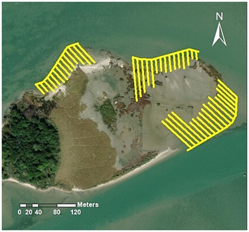
Figure 3. Location of transects used for Digital Shoreline Analysis System (DSAS, Table 3) analysis of change in shoreline position over time. Map image is the intellectual property of Esri and is used under license.

2.3 Adaptive management

In response to extensive plant mortality in the first season, an additional round of planting was conducted in June 2021. Due to budget constraints, this secondary planting was limited to the portion of the island deemed most susceptible to erosion and involved two components: (1) a larger area (4,780 m²) planted in traditional grid design with 0.46 m spacing between plugs; and, (2) a smaller experimental area (13 × 20 m grid, 260 m²) planted in a “clumped” design with 9 plugs clumped together and individual clumps spaced on a 1-meter grid. In total, 22,000 additional 5 cm plugs of S. alterniflora were installed.

3 Results

3.1 Topography

Prior to sediment placement, the interior region of the island was a mosaic of S. alterniflora marsh and subtidal habitat (Figure 4). A 2015 survey of the island commissioned by the USACE Baltimore District indicated that elevation of the intertidal regions within the project footprint varied from-0.2 to 0.4 m NAVD88, while elevations of the subtidal regions ranged from-0.43 to-0.31 m NAVD88. Sediment application resulted in elevation gains that ranged from ~0.15 m to >0.5 m and resulted in the entire project area being raised to a minimum of 0.2 m NAVD88. Analysis of the SfM-generated Digital Elevation Model (DEM) from 2019 indicated that areas that were intended to serve as high marsh were raised to an average elevation of 0.59 m while those areas intended to serve as dune habitat were raised to average elevations of 0.63 m (Dune East) and 0.89 m (Dune West).

Figure 4

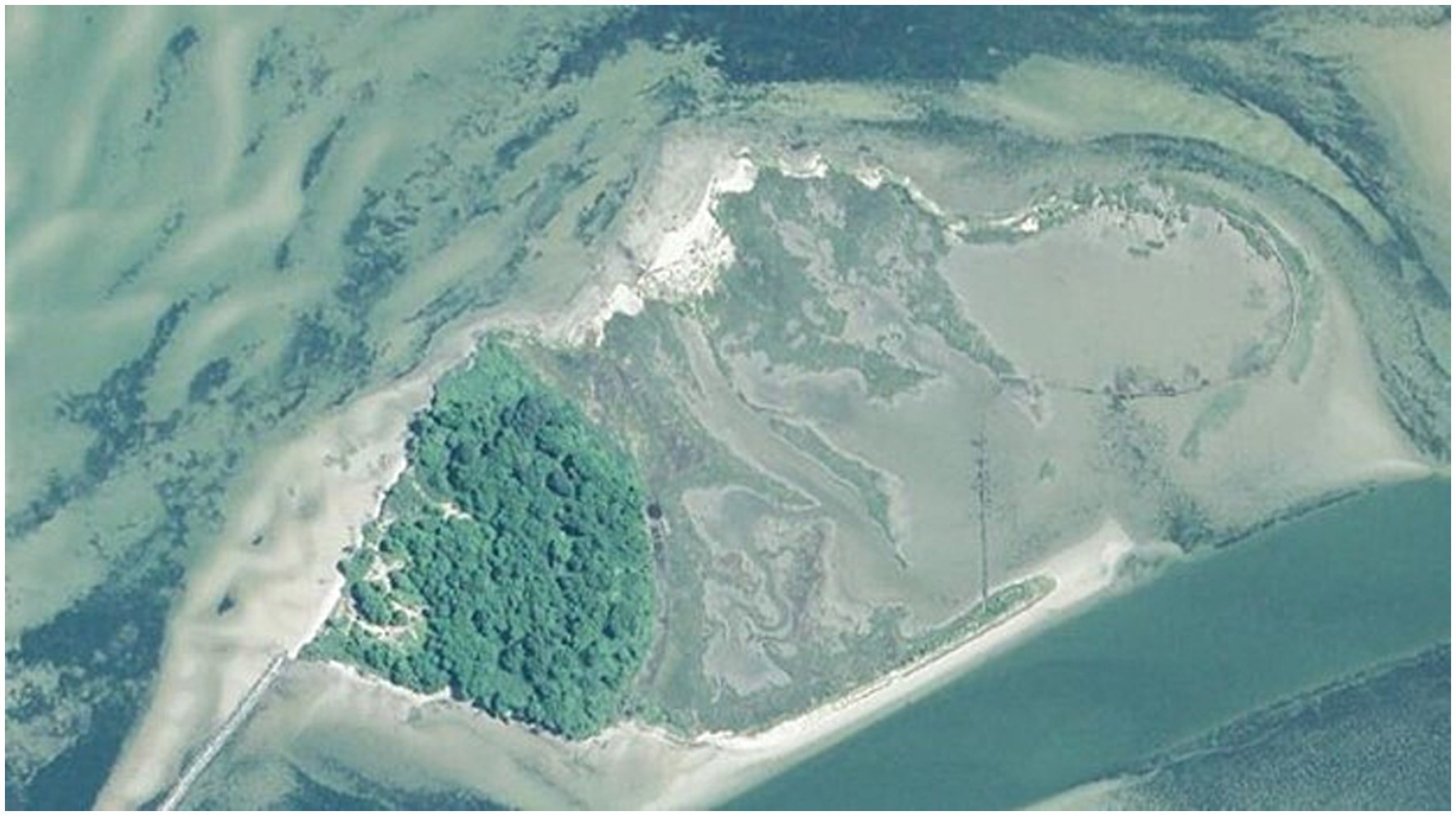
Figure 4. Pre-placement aerial imagery of Swan Island (2018) indicates a highly fragmented marsh with large areas of sparsely vegetated subtidal habitat within the “bight.” Image courtesy of Virginia Institute of Marine Science.

Changes in shoreline position and island topography over time were quantified by comparisons among SfM-generated DEMs (modeled elevations) as well as by among-year comparisons of the GPS measured elevations at each of the fixed sampling points. The positional accuracy of all SfM-generated DEMs was estimated based on the 2019 DEM by comparing the modeled and true positions of 12 checkpoints (Davis et al., 2022), to be 2.9 cm (X), 3.4 cm (Y) and 2.8 cm (Z). Comparison of DEM-modeled and GPS-measured elevations across all fixed sampling plots in all years indicated good agreement between the two approaches in unvegetated areas, but not where dense vegetation was present. Averaged over all post construction data collections (2020–2022), the Root Mean Square Error between modeled and measured elevations was 5.6 cm in unvegetated plots and 47 cm in vegetated plots. The large difference in DEM accuracy between bare ground and vegetated regions is expected in SfM-generated DEMs as the vegetative canopy obscures the sensor’s ability to “see” the ground surface (Davis et al., 2022) and thus to model it accurately.

Analysis of variance of GPS-measured fixed monitoring plot elevations by year in each planting zone indicated that post-placement sediment surface elevations were stable in vegetated zones (Dune West and High Marsh; Table 2). The only exception to this was for plots that were located on the shoreward edge of the western dune region where shoreline erosion resulted in significant losses in elevation. In contrast, the Dune East and Low Marsh regions, which were largely unvegetated, both lost elevation over time.

Table 2

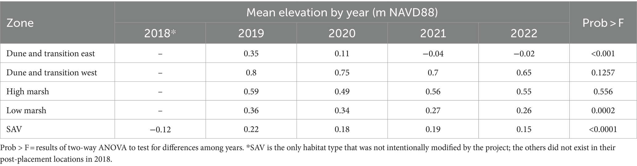
Table 2. Measured elevation averaged across all fixed monitoring plots in each planting zone.

In 2018, the average elevation across all SAV plots was -0.12 m NAVD88. During sediment-placement activities, dredged material that flowed across the coir-log barrier (which was designed to protect the SAV beds to the south), increased elevations within the bight by ~30 cm resulting in an average elevation of 0.18 m NAVD88 and burial of the existing SAV community.

Year-to-year comparison of SfM-generated DEMs highlights topographic changes in the island surface and the ingrowth of vegetation over time (Figure 5). Visual analysis of changes in the topography across the unvegetated platform highlights some consistent trends among years. First, the northern shoreline of Swan Island is eroding. This trend is particularly noticeable along the eastern stretch that falls behind the sill. Second, the material used to create the eastern dune appears to have migrated toward the southern shoreline and by 2022, to have been lost to the system entirely. Finally, the central portion of the placement area appears to be losing elevation across the full north to south extent of the island. One side effect of this loss in elevation is that the previously SAV-colonized bight on the southern side of the island is also losing elevation over time.

Figure 5

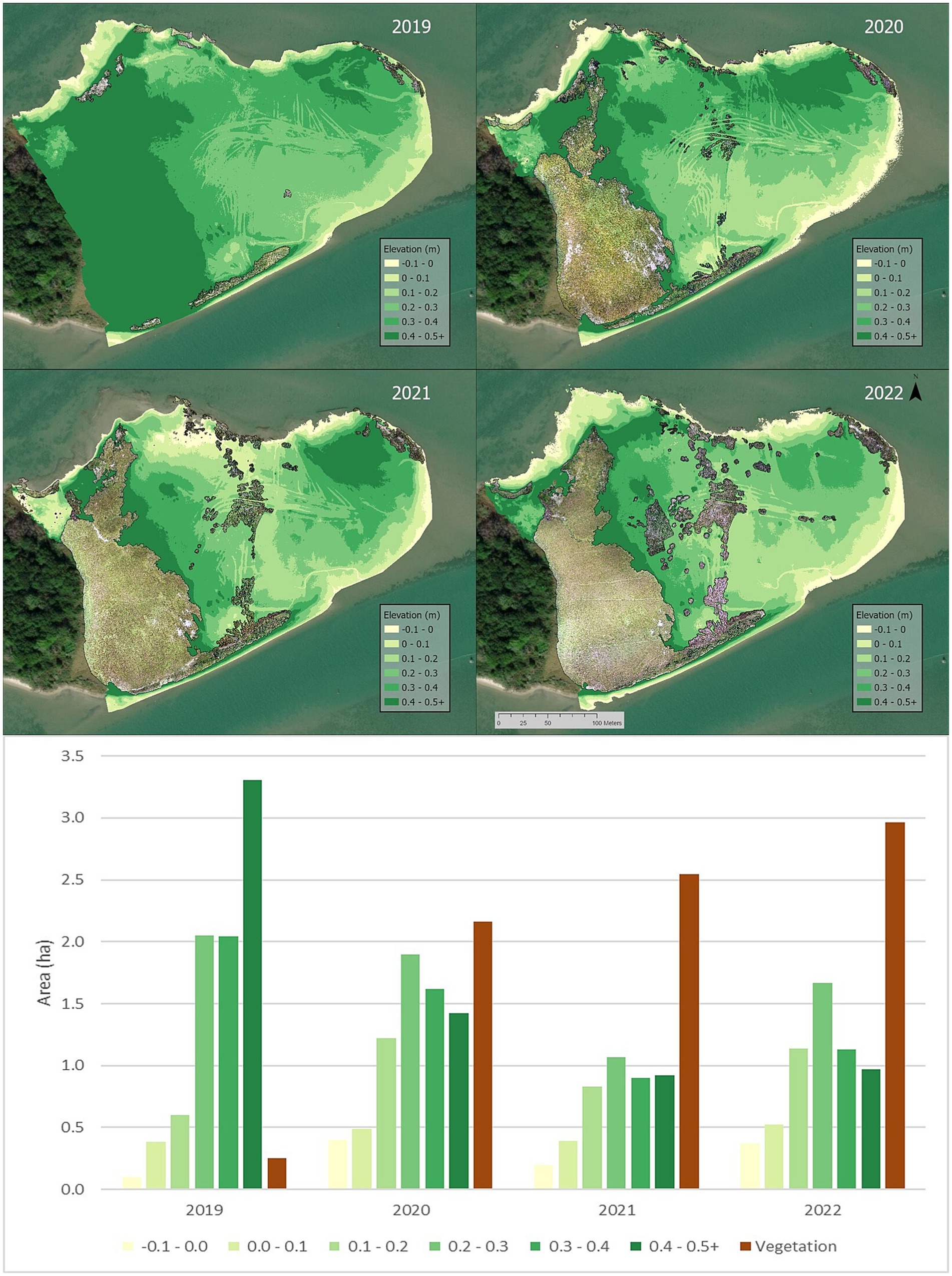
Figure 5. Topography and extent of vegetation by year determined from analysis of UAS-generated orthomosaic images and associated 3D surface models. Graph shows total extent of project area within each elevation bin by year. The elevation bins correspond to the ranges illustrated in the 4 image panels above. All elevation values are in units of m NAVD88.

3.2 Shoreline change rate

Average rates of shoreline change for each shoreline region calculated using the End Point Rate (EPR) method ranged from -3.08 to-4.02 m per year among regions (Table 3). These values are similar to those reported previously for the northwest region (Perini Management Services, 2014) and indicate that the island shorelines continue to contract. The Net Shoreline Movement (NSM; total change over the full 3-yr time period) varied by up to an order of magnitude among transects within the same region highlighting the very dynamic nature of this shoreline.

Table 3

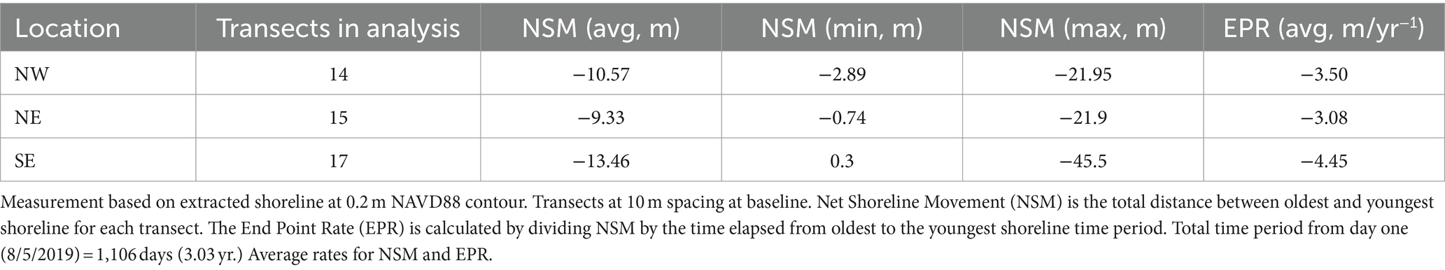
Table 3. Shoreline change rates by location: NE = Northeast, NW = Northwest, SE = Southeast.

3.3 Vegetation

Analysis of S. alterniflora biomass across the full elevation gradient at which it occurred prior to sediment placement indicated that average total standing biomass ranged between 88 and 572 g/m² and was greatest at elevations between 0.1 and 0.3 m NAVD88. Plot-averaged stem heights ranged between 52 and 137 cm and were greatest at elevations <0 m NAVD88.

After placement and planting, regions of the placement area at elevations >0.55 m NAVD88 were rapidly colonized by the planted S. patens. During the initial post-placement monitoring (August 2019), high marsh plots were characterized by total vegetative cover of <2% and average stem heights of 27 cm. By September of 2020, this area was densely colonized; most monitoring plots exhibited >50% cover with S. patens and maximum canopy heights (measured as the average of the 5 tallest stems in each plot) averaged 105 cm across all plots (Table 4). Since that time, the vegetative canopy in the high marsh has been consistently dense and slowly expanding toward the north and east. In areas of the island with marsh surface elevations <0.5 m NAVD88 that were planted with S. patens, the majority of the plantings were highly stressed or already dead by October 2019. By September of 2020, there was no longer any sign that planting had ever occurred in these areas, and large portions remained unvegetated as of 2022 (Figure 5, 2022).

Table 4

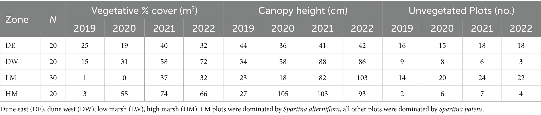
Table 4. Vegetative characteristics averaged across all fixed monitoring plots in each planting zone.

Due to the highly fragmented condition of the pre-existing marsh, the depth of applied sediments required to bring the island surface to the target elevation for low marsh was highly spatially variable. In areas where the depth of placement resulted in complete burial of the existing vegetation, the plants appear to have been smothered and there is no evidence of regrowth. In areas of the existing S. alterniflora marsh that were relatively high in elevation before the placement, sediment application did not result in complete burial of the vegetation; small clumps of S. alterniflora that survived the sediment placement were evident in the center of the island in August 2019. These patches of vegetation have been slowly expanding laterally since that time and appear to be the source of much of the vegetation that is currently present at elevations <0.5 m NAVD88 (Figure 6). The areas that were intended to be low marsh habitat but that remain unvegetated are characterized by elevations <0.5 m and by having been originally planted with S. patens.

Figure 6

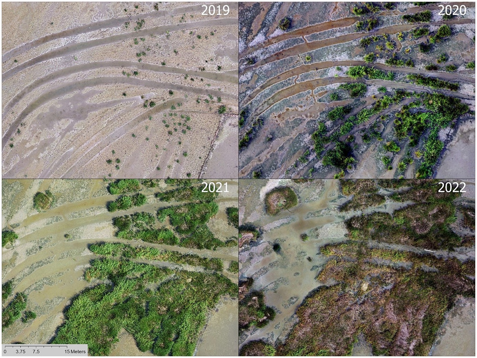
Figure 6. Analysis of UAS image orthomosaics illustrates expansion over time of low marsh vegetation that survived the initial deposition.

Average canopy height in plots occupied by S. alterniflora increased from 23 cm in 2019 to 103 cm in 2022 (Table 4). Despite a significant amount of ingrowth of S. alterniflora due to vegetative spread, most of the fixed low marsh plots (22 out of 30) remained unvegetated 3 years after the placement and planting.

We note that in 2022, a significant portion of the vegetated low marsh appeared to be senescent as evidenced by brown and brittle above-ground biomass (Figures 6, 7, 2022). This dieback was most pronounced in areas where a dense vegetative canopy had been present in 2021; there was little sign of dieback in recently colonized areas or in the area that was replanted in 2020. There was no evidence of a similar trend in plant communities other than S. alterniflora.

Figure 7

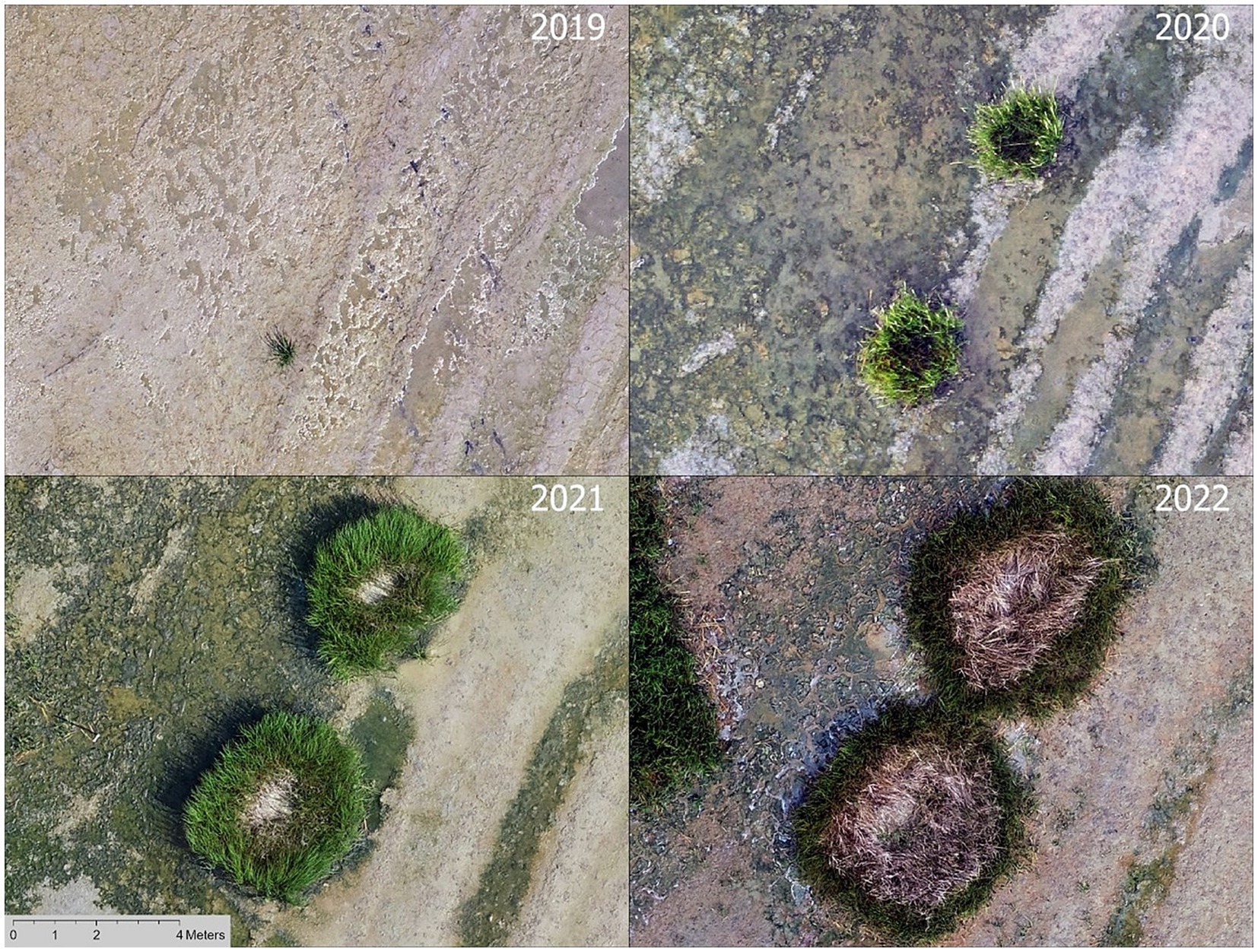
Figure 7. UAS image-generated orthomosaics illustrate growth of circular marsh tussocks from a few individual plants.

By August 2022, the replanting effort undertaken in 2021 was exhibiting variable results. In the southeastern portion of the re-planted area (lowest elevation and farthest from the shoreline), the new plantings were thriving and there was not a visible difference in plant density or morphometry among the plants that were clumped vs. not clumped (Figure 8). In the northern part of the planting area (closest to the shoreline), the new plantings failed to thrive and most of that area remained unvegetated as a result. The notable exception to this pattern was a dense stand of S. alterniflora that was present directly adjacent to the S. patens edge.

Figure 8

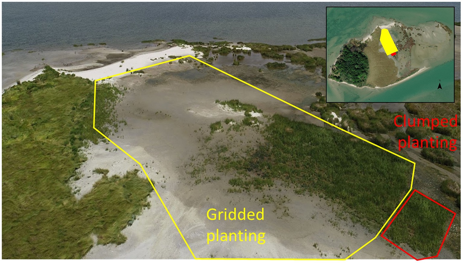
Figure 8. Additional areas of S. alterniflora planted in 2021 as part of the adaptive management action. Image taken in 2022.

The highest ridge of the western dune region has been densely colonized by Ammophila breviligulata (American beachgrass) through ingrowth of plants that survived the original deposition event. On the landward side of the dune ridge, A. breviligulata transitions to S. patens at elevations less than or equal to 0.8 m NAVD88 and percent vegetative cover of this region has steadily increased over time (Table 4). Planted S. patens on the eastern dune failed to thrive and, aside from some patches of S. alterniflora that have colonized low-lying pockets, the eastern dune region remained unvegetated as of 2022.

Prior to sediment placement, R. maritima was documented in 20 of the 21 monitoring plots (Table 5) in the subtidal bight, with total percent cover in each plot ranging from 2 to 85% (average = 43%) and canopy heights ranging from 3–13 cm. Reproductive structures (flowering shoots) were observed in 8 of the plots. After placement, R. maritima when present, occurred at greatly reduced percent cover (Table 5). No reproductive structures were observed in the years following sediment placement.

Table 5

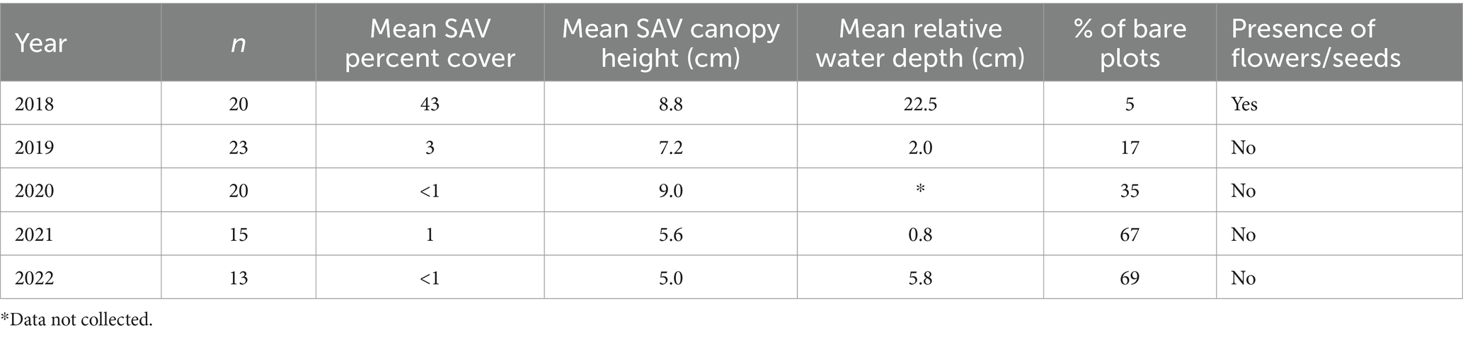
Table 5. SAV presence and percent cover over time.

In 2021, multiple patches (approximately 1 m²) of low-growing vegetation (presumptively identified as Liliaeopsis chinensis; eastern grasswort) began forming in the bight area. By 2022, these patches had coalesced into nearly continuous coverage across an area of approximately 2,850 square meters that was visible in aerial imagery. Comparison of modeled SAV plot elevations between years indicated an average decrease of 7.0 cm (+/− 2.2 cm) between 2019 and 2022 (Table 2).

3.4 Vegetation/topography feedbacks

By 2020, a large number of circular patches of marsh had begun to form in the central part of the island. Many of these patches appear to have grown from the vegetative spread of one or a few S. alterniflora plants (Figure 7). Over time, as these patches of marsh have expanded laterally, their interior elevations have increased by 20 cm or more, and in many, the centers are either unvegetated, or vegetated by species other than S. alterniflora. In 2022, we observed A. breviligulata and Cakile edentula (American searocket) growing in the center of several of the larger patches, indicating that some of these features have trapped enough sediment to outgrow intertidal marsh elevation.

3.5 Sediments and porewater

In 2018, prior to sediment placement, bulk density in the top 10 cm of existing sediments ranged from 0.2 to 1.5 g cm⁻³. The lower values were observed at optimal elevations for S. alterniflora growth (0 to 0.3 m NAVD88) with higher bulk densities, indicating greater sand content, observed at elevations above and below this range. After placement, average sediment bulk density in the top 10 cm was higher (1.44 ± 0.02, 1.34 ± 0.02, and 1.28 ± 0.03 g cm⁻³ in 2019, 2021 and 2022, respectively).

Due to the increase in sediment surface elevation after placement, we were only able to extract porewater from plots that were at lower elevations. In total, we collected 11 porewater samples in 2018 and 13 samples in 2019. Porewater NH₄ concentrations (averaged across all sample plots) increased from 83 μM in 2018 to 362 μM in 2019 while average PO₄ increased from 0.5 to 4.5 μM. There was no detectable relationship between either constituent and marsh surface elevation. Average porewater H₂S decreased from 6.2 to 0.87 mM between 2018 and 2019.

3.6 Wind and water levels

Analysis of Bishops Head water level data indicated that while annual average hourly water levels were similar among years (0.12, 0.08 and 0.09 m NAVD88, respectively, in calendar years 1 [2019–2020], 2 [2020–2021] and 3 [2021–2022]), the maximum water levels detected in years 1 and 3 (1.0 and 1.2 m NAVD 88) exceeded that of year 2 (0.8 m NAVD88). Analysis of wind data from 2019–2022 indicated that wind speeds and direction were similar among years (Figure 9). There were no major storm events evident in the wind data during this time (i.e., no measured sustained wind speeds in excess of 28 m/s). On average, wind speeds were between 4 and 5 m/s, and the maximum sustained wind speeds were between 15 and 23.6 m/s with that highest measured value occurring for 6 h on August 4, 2020. Occurrence of the strongest winds (>10 m/s) were mostly from the northwest which also happens to be the direction of maximum fetch. Water levels exceeding the top elevation of the sill structure occurred 2 to 3 times more frequently in years 1 and 3 than in year 2. The Bishops Head water level station is 22.5 km directly north of Swan Island and is located on the eastern shoreline of Chesapeake Bay. The use of Bishops Head water level trends as a proxy for conditions experienced at Swan Island is based on our assumption that this station experiences similar weather conditions, wind speeds, and directionality to Swan Island. While these assumptions have not been rigorously tested, Bishops Head water levels were found to be more conservative (lower) than the next closest long-term water level station (Lewisetta; LWTV2–8635750), on the Bay’s western shore and 13 km farther than Bishops Head.

Figure 9

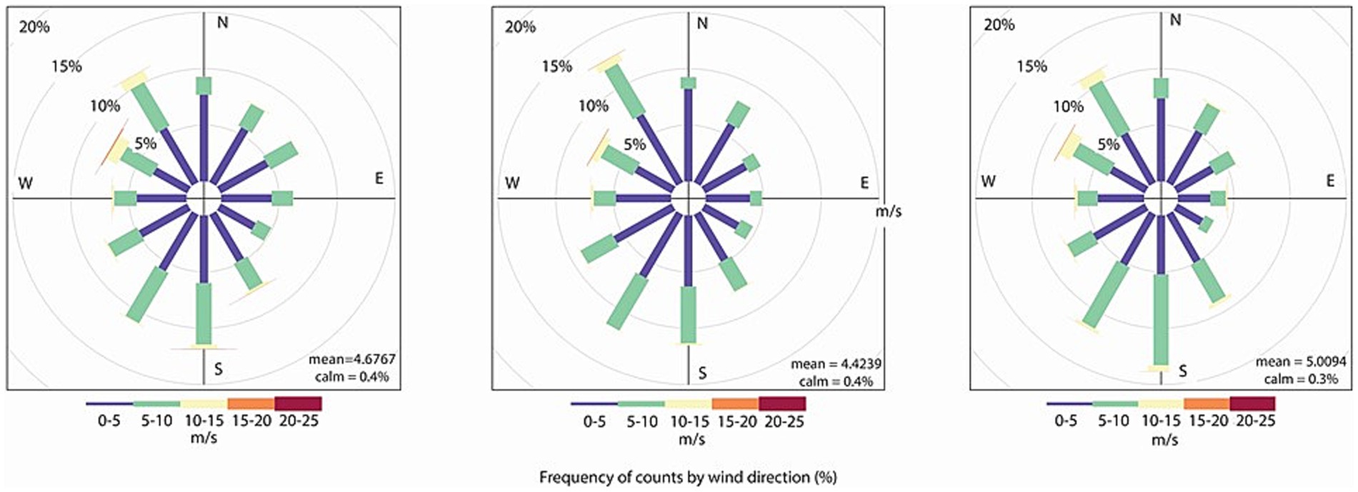
Figure 9. Wind roses for sampling year 1 (left), 2 (middle), and 3 (right) Illustrate ranges of wind speed frequency and direction during each year.

The peak elevation of the shore-parallel sill installed on the northeastern shoreline varies between 0.3 and 0.35 m NAVD88 along its length. This elevation is ~14 cm above the published value of MHW at this site (0.21 m NAVD88) according to tidal datums estimated by NOAA’s VDATUM tool.¹ We note that the datums currently used by VDATUM are relative to the 1983–2001 tidal datum epoch. Monthly datums for Bishops Head were averaged for each consecutive 12-month period from August 1, 2018 through July 31, 2022. These annually averaged values of MHW ranged from a low of 0.35 to a high of 0.38 m NAVD88, indicating that the published datums were not representative of conditions experienced on the ground during this period. Analysis of hourly water level data at Bishops Head over the 3-year monitoring period suggests that water levels exceeded sill height for significant periods of time (on the order of 8 weeks cumulatively in year 1 alone; Table 6).

Table 6

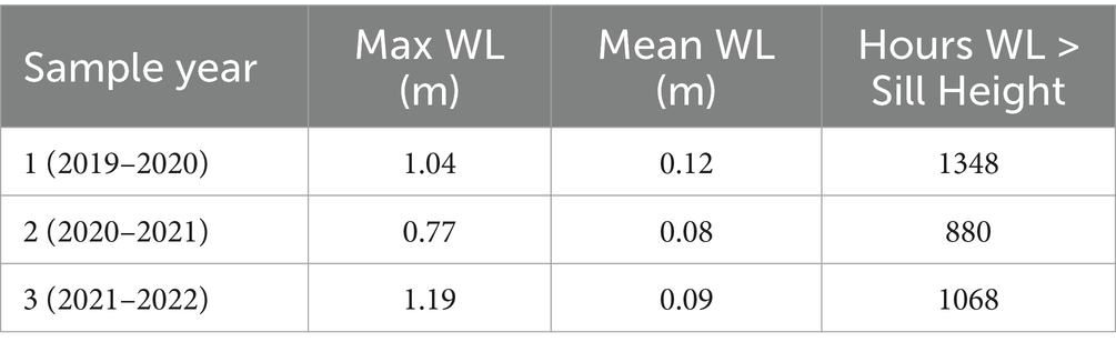
Table 6. Average water level (WL; relative to NAVD88) at bishops head by sample year.

4 Discussion

Sediment placement at Swan Island converted the eastern two thirds of the island from a highly fragmented low marsh into a more diverse system that includes dunes and high intertidal marsh habitat. The working assumption was that incorporation of a wider range of surface elevations in this portion of the island would result in a feature with enhanced biodiversity (Meli et al., 2014) that would be more resilient to future sea level rise and remain effective as a wave shield for the downwind shoreline of Ewell, MD. There is no current effort to track island-wide biodiversity however, it is assumed that creating a wider range of habitat types than was initially present will result in a greater diversity of species present. An ongoing simulation modeling-based effort to evaluate the role of Swan Island as a wave break suggests that the latter assumption is correct (Tritinge and Dillon, in press). The extent to which the sediment placement action will ultimately translate into increased resilience to sea-level rise remains to be seen and based on our findings, is likely highly dependent upon vegetative colonization of the portions of the island that are currently unvegetated. Our continued monitoring efforts at this site will shed light on the changes that occur as the system matures. In the short term, the early monitoring data reported here yield valuable insights that can be applied to future projects and inform the growing discussion about how and where natural infrastructure strategies can be used with predictable results.

4.1 Stability of placed sediments

Three full years after construction, there has been no detectable change in surface elevations in regions not impacted by erosion (i.e., Dune West and High Marsh zones; Table 2). This finding indicates that neither consolidation of the placed sediments nor compaction of the underlying sediments has occurred at measurable rates. This is likely a function of the high sand content in both the underlying and applied sediments at Swan Island, as sand is not highly compressible (Mudd et al., 2009). Despite the apparent resistance of the placed sediments to settling over time, a general trend of decreasing surface elevation was observed across unvegetated regions of the island. This loss of elevation appears to be due to the erosion of sediments from the surface and has resulted in a net loss of material from the island platform based on comparison of annual DEMs.

The sill structure that was installed parallel to the northeast shoreline (Figure 1) has not been effective in stabilizing the area behind it. Guidance for living shoreline sill design suggests that in moderate wave energy settings, sills be built to 30 to 60 cm above MHW (VIMS, n.d.). The sill crest at Swan was roughly 14 cm above published MHW (but approximately even with MHW measured during the sampling period), which appears to be too low to provide adequate protection. Analysis of water level trends at the Bishops Head station indicated that the sill was inundated for a cumulative 2 months in the first year alone, at times by as much as 20–30 cm. Ultimately, the combination of low sill height and failure of the plantings to become established left this area undefended against erosion and resulted in loss of the created dune feature.

Prior to restoration, the long-term (1942–2013) rate of change on the northwest facing shoreline of Swan Island was -1 to -4 m/yr (Perini Management Services, 2014). Post-restoration, the average rate of change along the northern shoreline was -3.3 m/yr. That the placement of unconsolidated sediments did not reduce wave energy-driven erosion on the northern shoreline is not surprising. Wave action on the placed sediments appears to be fueling a slow north to south migration of sediment across the surface of the island. This trend is most apparent on the eastern lobe of the island where there is little vegetation to impede the movement of sediments (or to obscure our ability to detect changes via the SfM-derived DEMs). It appears that much of this migrating sediment may ultimately be carried back into the channel to the south, representing a net loss of volume for the island.

4.2 Success of vegetative plantings

While the total area of vegetated marsh has increased over time, the pace of vegetative ingrowth has been slow throughout the lower elevation areas. As of 2022, the cumulative extent of vegetated intertidal platform (including all three target habitat types) at Swan Island was comparable to pre-placement conditions (2018 = 33,500 m², 2022 = 32,000 m² [20,000 m² high marsh, 12,000 m² low marsh]). Roughly 15,000 m² of island surface area that was designed to support low marsh remained unvegetated as of 2022. Most of that area was still within the range of elevations that is appropriate for S. alterniflora. Thus, it is anticipated that over time, as long as the pace of vegetative spread outpaces the rate at which elevation is lost to erosion, the total extent of vegetated marsh platform will continue to increase.

Vegetative success at Swan Island varied by species and planting elevation. While S. patens thrived when planted at elevations above 0.55 m, it failed when planted below that elevation. Much of the S. alterniflora planted in 2019 failed to thrive even when planted at elevations that were previously shown to be optimal for its growth on Swan Island (~0.3 m NAVD88). Results were mixed for the S. alterniflora that was planted in 2021 as part of the adaptive management action. In that case, the new plantings grew vigorously in the southeastern portion of the planting area but failed to thrive in the more northern region of the planting area.

Previous manipulative experiments have demonstrated survival of marsh plantings to be impacted by elevation, salinity, plant source (native vs. greenhouse grown), timing of planting, soil redox status, nutrient availability, and competitive interactions with other species (Broome et al., 1988; Burchett et al., 1998; Konisky and Burdick, 2004; O’Brien and Zedler, 2006; Beck and Gustafson, 2012). In short, there are a myriad of factors that can impact vegetative success and it can be difficult to discern the reason for sub-optimal results on any given project. In a systematic review of coastal ecosystem restoration efforts, Bayraktarov et al. (2015) estimated the median short term (1–2 year) survival rate of marsh plantings to be 65%. This finding highlights the inherent uncertainty associated with vegetative community establishment and the need to plan for adaptive management actions.

In the current study, it is clear that when S. patens failed to thrive, it was the result of being planted at sub-optimal elevations. The drivers of S. alterniflora success at Swan Island are less clear, and are partially confounded by recolonization of some regions by existing plants that survived the deposition. Inspection of the UAS imagery time series suggests that aside from the adaptive management planting area, the contribution of planted S. alterniflora to the current total areal extent of this species is negligible. Average post-placement sediment bulk density in the low marsh zone, while elevated relative to average pre-placement values, was within the range of values at which S. alterniflora was documented before the placement action and thus, appears to be appropriate for growth. Site managers did observe grazing by geese on some of the new plantings, but this did not appear to be extensive. The documented increase in porewater nutrient concentrations between 2018 and 2019 suggests that the placed sediments provided a source of nutrients to fuel plant growth. Measured post-placement concentrations of NH₄⁺ and PO₄, while below those documented at nearby dredge-material created Poplar Island, were within the range measured in natural tidal marshes of Chesapeake Bay (Stevenson and Kearney, 2009; Cornwell et al., 2020) suggesting that plant establishment was not limited by nutrient availability.

The adaptive management planting conducted in 2021 targeted an area of 5,040 m². Of that area, approximately 20% was densely colonized by vegetative spread of the planted plugs within one year. The plantings that were successful were either: part of the clumped planting grid; farthest from the actively eroding northern shoreline (i.e., the southeastern corner of the planting grid); or directly adjacent to the landward edge of the densely vegetated S. patens zone (Figure 8) and thus shielded from direct wave energy. Many uprooted but intact plugs were observed lying on the marsh surface in August 2021; these appeared to have been dislodged by wave action. We thus hypothesize that water flow (and associated sediment movement) across this region was the driving force behind failure of plantings in the northern portion of the adaptive management planting area. There was no observable relationship between planting success and elevation in the adaptive management plantings, and no indication that clumped planting provided any advantage over gridded planting in this region.

The development of circular S. alterniflora mounds or “tussocks” (Figure 7), is further indication of the energetics of this region. Growth and evolution of such tussocks have been previously documented for Spartina spp. colonizing tidal mudflats (Sánchez et al., 2001; Ward et al., 2003; Balke et al., 2012). In these largely unvegetated platforms, the successful establishment of a small patch of plants has a very localized effect of dampening wave energy which leads to sediment deposition within the vegetated clump. This process results in the outward spread of clumps and eventually, in the formation of dome shaped mounds (tussocks) of vegetation. Hydrological energy in the form of both waves and currents has been shown to interact with the plant density/sediment trapping relationship to influence the lateral expansion of tussocks (Duggan-Edwards et al., 2019). Specifically, higher wave energy settings tend to lead to greater sediment availability via erosion and thus higher mounds, but depressions or “erosion gullies” tend to form adjacent to these mounds, effectively slowing their outward expansion (Bouma et al., 2009). In the case of Swan Island, the formation of tussocks without gullies seems to indicate moderate levels of hydrodynamic energy even in the interior regions of the island and lends credence to the hypothesis that success of the adaptive management plantings was limited by hydrodynamic energy.

The observed die-back of vegetation in 2022, the third growing season after planting, mirrors a trend previously reported at the Poplar Island restoration site further north in Chesapeake Bay. There, planted vegetation expanded rapidly in the first two years, reaching maximum values of biomass by year 2, followed by an unexpected die back of vegetation in large areas of previously thriving marsh by year 3. Additional plantings conducted within the die-off zone showed 100% survival indicating that dieback was not the result of inhospitable conditions for growth. The cause of that event has not been satisfactorily determined but the marsh recovered and stabilized within the next few growing seasons (Staver, 2015). At Swan Island, examination of the imagery time series indicates that vegetation that was green in 2022 (year 3) was not present in 2021, conversely all areas of the low marsh that were vegetated in 2021 were brown and dead in 2022. This trend is clearly evident in the vegetated tussocks where green vegetation (in 2022; Figure 7) represents the outward expansion of the mound. While the cause of the dieback at Swan Island is not known, it does appear to be following the pattern detected at Poplar Island, thus we anticipate recovery in 2023, potentially followed by rolling age-based diebacks as vegetative cover continues to expand.

In 2021, US Fish and Wildlife Service scientists conducted bird surveys on Swan Island and in a nearby reference marsh using standardized protocols established by the Saltmarsh Habitat and Avian Research Program (SHARP–saltmarsh habitat and avian research program, 2017). The primary difference noted between Swan Island and reference sites was a greater abundance of salt-marsh obligate species (clapper rails and seaside sparrows) in the reference marsh (Whitbeck, unpublished data). The difference is presumably due to large portions of the Swan Island survey plots being unvegetated. While not surprising, these observations highlight the fundamental role that vegetative community establishment plays not only in island stabilization but also in achieving habitat goals.

4.3 Impacts on SAV

The coir log structure, installed to form a protective barrier to sediment movement between the placement area and the SAV bed to the south (Figure 1, bottom), was not effective in limiting the spread of sediment into the bight. The material that leaked across this structure ultimately buried over 2 acres of SAV habitat by an average depth of 30 cm. The initial hypothesis was that this material would be rapidly removed by tidal action due to the lack of vegetative canopy present to stabilize it. Between 2019 and 2022, the average sediment surface elevation within the previous SAV bed decreased by 8 cm. The elevation profile within that region is undoubtedly influenced by inputs of new sediments which are eroding from the northern shoreline and migrating southward across the island surface. In the last two years, a large portion of this area has been colonized by Liliopsis chinensis, a common inhabitant of brackish intertidal mudflats. Development of this patch seems to signify that conditions are stabilizing within the bight region, but at higher elevations not suitable for SAV.

4.4 Lessons learned (so far)

Data from the first three years post-construction show that Swan Island continues to evolve as it matures. The lessons learned to date provide a glimpse into the challenges and benefits of using dredged material to increase resilience of coastal habitats. Efforts like the restoration of Swan Island that involve the targeted and strategic reuse of sediments to create or re-create small-scale features require a high degree of precision which can be challenging to achieve given the current state of sediment placement technology, and the inherent unpredictability of the environmental forces that influence restoration outcomes.

At Swan Island, the as-built project closely mirrored the planned design and has largely continued to do so since implementation. The northern shoreline of Swan Island faced significant erosion in the past and the forces acting on that area were not significantly changed by the restoration. It should therefore come as no surprise that the north shoreline continues to erode at rates similar to those that were prior to restoration. It seems likely that better immediate success of the vegetative plantings would have helped to minimize change along this shoreline, particularly in the stretch of shoreline behind the sill. Clearly, some amount of hardening (shoreline rip rap or offshore sill) would be necessary to stop erosion of the northern shoreline, although it may be more cost effective to consider repeat sediment placements than to build hard structures.

It is worth noting that the ability to grade with heavy machinery to achieve desired elevations and to plant vegetation by hand (which was possible because of the manageable project size) may render this site somewhat unique. In cases where the placed material cannot be graded with such precision, reaching target elevations will be much more challenging. The planting and failure of S. patens in large areas of the island that were below this species’ elevation threshold highlight the need for a thorough understanding of both the inundation regime and inundation tolerance of target species within the local tidal regime.

Creating a thriving wetland habitat that is resilient to future sea-level rise requires creating the right conditions for vegetative growth. This is demonstrated by the consistency in elevation of the densely vegetated high marsh platform over time, and in the low marsh tussocks where the vegetation is effectively trapping sediment and holding it in place. As previously noted, vegetation can fail to become established for a wide variety of reasons including anomalous weather events that are impossible to predict. As a result, at sites like Swan Island where there is enough wave energy that vegetation is required to hold the sediments in place, it is advisable to have not only a plan for adaptive plantings, but also an identified source of funding to make it possible. While having an adaptive management plan does not guarantee project success, it greatly increases the likelihood.

The burial of the existing SAV bed was an unfortunate and unintended consequence of the sediment placement action. The potential for burial was also one of the greater concerns of resource management agencies involved with permitting this project. The lack of short-term SAV recovery emphasizes the significance of post-project monitoring and the need for an adaptive management plan that includes adjacent habitats. Avoiding unintended impacts to these adjacent habitats through adequate control measures is essential to maintaining the integrity of these interconnected ecosystems and ensuring overall project success. The results of this effort indicate that coir logs alone are not sufficient to contain sediment. It is worth noting that the transition of SAV habitat to mudflat does not equate to a complete loss of habitat value; this area currently serves as feeding ground for a range of shorebirds.

Beneficial use of sediments to create natural infrastructure is a relatively new practice and, as such, comes with some uncertainty. At Swan Island, the burial of subtidal SAV habitat via leakage of sediment through the coir log barrier and failure of a portion of the initial plantings were unintended outcomes. With these uncertainties come opportunities, such as keeping sediment in the system, prolonging Island longevity, creating much needed bird habitat in the face of sea level rise, and providing a guide for future projects (Whitfield et al., 2022). Even though there may be unforeseen effects, having a plan, and a means of conducting adaptive action early in the process will reduce uncertainty in ultimate outcomes.

Data availability statement

The raw data supporting the conclusions of this article will be made available by the authors, without undue reservation.

Author contributions

JD: Conceptualization, Funding acquisition, Investigation, Methodology, Project administration, Writing – original draft, Writing – review & editing. PW: Conceptualization, Funding acquisition, Project administration, Writing – original draft, Writing – review & editing. RyG: Data curation, Formal analysis, Investigation, Methodology, Visualization, Writing – review & editing. ReG: Conceptualization, Formal analysis, Investigation, Project administration, Writing – original draft, Writing – review & editing. MG: Data curation, Formal analysis, Investigation, Methodology, Visualization, Writing – review & editing. LP: Data curation, Formal analysis, Investigation, Visualization, Writing – review & editing. MW: Data curation, Investigation, Writing – review & editing.

Funding

The author(s) declare financial support was received for the research, authorship, and/or publication of this article. Funding for this project comes from NOAA’s National Centers for Coastal Ocean Sciences and U.S. Army Corps of Engineers Engineering With Nature Initiative^®.

Acknowledgments

Brooke Landry, Molly Bost, Alyssa LeClaire, and Don Field helped with data collection and sample processing. MW and USFWS staff coordinated field efforts and facilitated site access for all research teams. This manuscript benefited from thoughtful reviews by Emily Russ, Justin Ridge, Tom Parham, and two reviewers.

Conflict of interest

RyG was employed by Consolidated Safety Services Inc.

The remaining authors declare that the research was conducted in the absence of any commercial or financial relationships that could be construed as a potential conflict of interest.

Publisher’s note

All claims expressed in this article are solely those of the authors and do not necessarily represent those of their affiliated organizations, or those of the publisher, the editors and the reviewers. Any product that may be evaluated in this article, or claim that may be made by its manufacturer, is not guaranteed or endorsed by the publisher.

Footnotes

1. ^https://vdatum.noaa.gov/

References

Balke, T., Klaassen, P. C., Garbutt, A., van der Wal, D., Herman, P. M. J., and Bouma, T. J. (2012). Conditional outcome of ecosystem engineering: a case study on tussocks of the salt marsh pioneer Spartina anglica. Geomorphology 153–154, 232–238. doi: 10.1016/j.geomorph.2012.03.002

Crossref Full Text | Google Scholar

Bayraktarov, E., Saunders, M. I., Abdulla, S., Mills, M., Beher, J., Possingham, H. P., et al. (2015). The cost and feasibility of marine coastal restoration. Ecol. Appl. 26, 1055–1074. doi: 10.1890/15-1077

PubMed Abstract | Crossref Full Text | Google Scholar

Beck, J., and Gustafson, D. J. (2012). Plant source influence on Spartina alterniflora survival and growth in restored South Carolina salt marshes. Southeast. Nat. 11, 747–754. doi: 10.1656/058.011.0412

Crossref Full Text | Google Scholar

Bouma, T. J., Friedrichs, M., Van Wesenbeeck, B. K., Temmerman, S., Graf, G., and Herman, P. M. J. (2009). Density-dependent linkage of scale-dependent feedbacks: a flume study on the intertidal macrophyte Spartina anglica. Oikos 118, 260–268. doi: 10.1111/j.1600-0706.2008.16892.x

Crossref Full Text | Google Scholar

Bridges, T. S., Lillycrop, J., Wilson, J. R., Fredette, T. J., Suedel, B., Banks, C. J., et al. (2014). Engineering with nature promotes triple-win outcomes. Terra et Aqua, 135, 17–23. Available at: https://ewn.erdc.dren.mil/wp-content/uploads/2021/03/2014_Terra-et-Aqua-EWN.pdf (Accessed December 19, 2023).

Google Scholar

Broome, S. W., Seneca, E. D., and Woodhouse, W. W. (1988). Tidal salt marsh restoration. Aquat. Bot. 32, 1–22. doi: 10.1016/0304-3770(88)90085-X

Crossref Full Text | Google Scholar

Burchett, M. D., Allen, C., Pulkownik, A., and MacFarlane, G. (1998). Rehabilitation of saline wetland, Olympics 2000 site, Sydney (Australia). II: saltmarsh transplantation trials and application. Mar. Pollut. Bull. 37, 526–534. doi: 10.1016/S0025-326X(98)00137-4

Crossref Full Text | Google Scholar

Burdick, D., and Kendrick, G. (2001). “Standards for seagrass collection, identification and sample design” in Global methods in seagrass research. eds. F. Short and R. Coles (Boston, MA: Elsevier Science), 79–100.

Google Scholar

Chausson, A., Turner, B., Seddon, D., Chabeneix, N., Girardin, C. A. J., Kapos, V., et al. (2020). Mapping the effectiveness of nature-based solutions for climate change adaptation. Glob. Chang. Biol. 26, 6134–6155. doi: 10.1111/gcb.15310

PubMed Abstract | Crossref Full Text | Google Scholar

Cline, J. D. (1968). Kinetics of the sulfide-oxygen reaction in seawater; an investigation at constant temperature and salinity. [M.S. Thesis]. [Seattle, WA]: Univ. Washington.

Google Scholar

Code of Maryland Regulations (COMAR) (1994). Dredging and Filling. 26.24.03. Available at: http://mdrules.elaws.us/comar/26.24.03 (Accessed December 19, 2023).

Google Scholar

Cornwell, J. C., Owens, M. S., Staver, L. W., and Stevenson, J. C. (2020). Tidal marsh restoration at Poplar Island I: transformation of estuarine sediments into marsh soils. Wetlands 40, 1673–1686. doi: 10.1007/s13157-020-01294-5

Crossref Full Text | Google Scholar

Davis, J., Currin, C., and Mushegian, N. (2022). Effective use of thin layer sediment application in Spartina alterniflora marshes is guided by elevation-biomass relationship. Ecol. Eng. 177:106566. doi: 10.1016/j.ecoleng.2022.106566

Crossref Full Text | Google Scholar

Davis, J., Whitfield, P., Szimanski, D., Golden, B. R., Whitbeck, M., Gailani, J., et al. (2021). A framework for evaluating island restoration performance: a case study from Chesapeake Bay. Integr. Environ. Assess. Manag. 18, 42–48. doi: 10.1002/ieam.4437

PubMed Abstract | Crossref Full Text | Google Scholar

DiGiacomo, A. E., Giannelli, R., Puckett, B., Smith, E., Ridge, J. T., and Davis, J. (2022). Considerations and tradeoffs of UAS-based coastal wetland monitoring in the southeastern United States. Front. Remote Sens. 3:924969. doi: 10.3389/frsen.2022.924969

Crossref Full Text | Google Scholar

Douglas, W. S., Yepsen, M. M., and Flanigan, S. (2021). Beneficial use of dredged material for marsh, dune and beach enhancement in a coastal New Jersey wildlife refuge. WEDA J. Dred. 19, 1–23.

Google Scholar

Duggan-Edwards, M. F., Pages, J. F., Jenkins, S. R., Bouma, T. J., and Skov, M. W. (2019). External conditions drive optimal planting configurations for salt mars restoration. J. Appl. Ecol. 57, 619–629. doi: 10.1111/1365-2664.13550

Crossref Full Text | Google Scholar

Erwin, M. E., Brinker, D. F., Watts, B. D., Costanzo, G. R., and Morton, D. D. (2011). Islands at bay: rising seas, eroding islands, and waterbird habitat loss in Chesapeake Bay (USA). Journal of Coastal Conservation, 27, 505. doi: 10.1007/s11852‐010‐0119‐y

Crossref Full Text | Google Scholar

Haskins, J., Endris, C., Thomsen, A. S., Gerbl, F., Fountain, M. C., and Wasson, K. (2021). UAV to inform restoration: a case study from a California tidal marsh. Front. Environ. Sci. 9:642906. doi: 10.3389/fenvs.2021.642906

Crossref Full Text | Google Scholar

Himmelstoss, E. A., Henderson, R. E., Kratzmann, M. G., and Faris, A. S. (2018). Digital shoreline analysis system (DSAS) version 5.0 user guide. Woods Hole, MA: U.S. Geological Survey. 1179. 1110.

Google Scholar

IPBES (2019). Global assessment report on biodiversity and ecosystem services of the intergovernmental science-policy platform on biodiversity and ecosystem services (version 1) Bonn, Germany: Zenodo.

Google Scholar

Konisky, R. A., and Burdick, D. M. (2004). Effects of stressors on invasive and halophytic plants of New England salt marshes: a framework for predicting response to tidal restoration. Wetlands 24, 434–447. doi: 10.1672/0277-5212(2004)024[0434:EOSOIA]2.0.CO;2

Crossref Full Text | Google Scholar

Landry, J. B., and Golden, R. R. (2018). In-situ effects of shoreline type and watershed land use on submerged aquatic vegetation habitat quality in the Chesapeake and mid-Atlantic coastal bays. Estuar. Coasts 41, 101–113. doi: 10.1007/s12237-017-0316-0

Crossref Full Text | Google Scholar

Marbán, P. R., Mullinax, J. M., Resop, J. P., and Prosser, D. J. (2019). Assessing beach and island habitat loss in the Chesapeake Bay and Delmarva coastal bay region, USA, through processing of Landsat imagery: a case study. Remote Sens. Appl. Soc. Environ. 16:100265. doi: 10.1016/j.rsase.2019.100265

Crossref Full Text | Google Scholar

McAtee, K. J., Thorne, K. M., and Witcraft, C. R. (2020). Short-term impact of sediment addition on plants and invertebrates in a southern California salt marsh. PLoS One 15:E0240597. doi: 10.1371/journal.pone.0240597

PubMed Abstract | Crossref Full Text | Google Scholar

Meli, P., Rey Benayas, J. M., Balvanera, P., and Martínez Ramos, M. (2014). Restoration enhances wetland biodiversity and ecosystem service supply, but results are context-dependent: a Meta-analysis. PLoS One 9:e93507. doi: 10.1371/journal.pone.0093507

PubMed Abstract | Crossref Full Text | Google Scholar

Morris, J. T., Sundareshwar, P. V., Nietch, C. T., Kjerfve, B., and Cahoon, D. R. (2002). Responses of coastal wetlands to rising sea level. Ecology 83, 2869–2877. doi: 10.1890/0012-9658(2002)083[2869:ROCWTR]2.0.CO;2

Crossref Full Text | Google Scholar

Mudd, S. M., Howell, S. M., and Morris, J. T. (2009). Impact of dynamic feedback between sedimentation, sea-level rise, and biomass production on near-surface marsh stratigraphy and carbon accumulation. Estuar. Coast. Shelf Sci. 82, 377–389. doi: 10.1016/j.ecss.2009.01.028

Crossref Full Text | Google Scholar

Nelson, D. R., Bledsoe, B. P., Ferreira, S., and Nibbelink, N. P. (2020). Challenges to realizing the potential of nature-based solutions. Curr. Opin. Environ. Sustain. 45, 49–55. doi: 10.1016/j.cosust.2020.09.001

Crossref Full Text | Google Scholar

NOAA National Centers for environmental information (NCEI). (2023). U.S. billion-Dollar weather and climate disasters. Available at: https://www.ncei.noaa.gov/access/billions/ (Accessed December 12, 2023).

Google Scholar

O’Brien, E. L., and Zedler, J. B. (2006). Accelerating the restoration of vegetation in a southern California salt marsh. Wetl. Ecol. Manag. 14, 269–286. doi: 10.1007/s11273-005-1480-8

Crossref Full Text | Google Scholar

Over, J. R., Ritchie, A. C., Kranenburg, C. J., Brown, J. A., Buscombe, D., Noble, T., et al. (2021). Processing coastal imagery with Agisoft Metashape professional edition, version 1.6—Structure from motion workflow documentation: U.S. Geological Survey open-file report 2021–1039, 46.

Google Scholar

Parsons, T. R., Maita, Y., and Lalli, C. M. (1984). A manual of chemical and biological methods for seawater analysis. Oxford, UK, Pergamon, Press. 173.

Google Scholar

Peet, R. K., Wentworth, T. R., and White, P. S. (1998). A flexible, multipurpose method for recording vegetation composition and structure. Castanea 63: 262–274.

Google Scholar

Perini Management Services. (2014). Study report, Smith Island, Martin National Wildlife Refuge. Hurricane Sandy Resiliency Project #31, Fog Point Living Shoreline Restoration.

Google Scholar

Puchkoff, A. L., and Lawrence, B. A. (2022). Experimental sediment addition in salt-marsh management: plant-soil carbon dynamics in southern New England. Ecol. Eng. 175:106495. doi: 10.1016/j.ecoleng.2021.106495

Crossref Full Text | Google Scholar

Raposa, K., Bradley, M., Chaffee, C., Ernst, N., Ferguson, W., Kutcher, T. E., et al. (2022). Laying it on thick: ecosystem effects of sediment placement on a microtidal Rhode Island salt marsh. Front. Environ. Sci. 10. doi: 10.3389/fenvs.2022.939870

PubMed Abstract | Crossref Full Text | Google Scholar

Raposa, K., Wasson, K., Nelson, J., Fountain, M., West, J., Endris, C., et al. (2020). Guidance for thin-layer sediment placement as a strategy to enhance tidal marsh resilience to sea-level rise. Published in collaboration with National Estuarine Research Reserve System Collaborative. Available at: https://nerrssciencecollaborative.org/resource/guidance-thin-layer-sediment-placement (Accessed December 12, 2023).

Google Scholar

Rodriguez, A. B., Fodrie, F. J., Ridge, J. T., Lindquist, N. L., Theuerkauf, E. J., Coleman, S. E., et al. (2014). Oyster reefs can outpace sea-level rise. Nat. Clim. Chang. 4, 493–497. doi: 10.1038/nclimate2216

Crossref Full Text | Google Scholar

Rosenzweig, C., Solecki, W., DeGaetano, A., O'Grady, M., Hassol, S., and Grabhorn, P. (Eds.) (2011). Responding to climate change in New York state: The ClimAID integrated assessment for effective climate change adaptation: Synthesis report. New York State Energy Research and Development Authority (NYSERDA), Albany, New York.

Google Scholar

Sánchez, J. M., SanLeon, D. G., and Izco, J. (2001). Primary colonisation of mudflat estuaries by Spartina maritima (Curtis) Fernald in Northwest Spain: vegetation structure and sediment accretion. Aquat. Bot. 69, 15–25. doi: 10.1016/S0304-3770(00)00139-X

Crossref Full Text | Google Scholar

SHARP–saltmarsh habitat and avian research program (2017). Available at: https://www.tidalmarshbirds.org/index.php (Accessed December 20, 2023).

Google Scholar

Spalding, M. D., Ruffo, S., Lacambra, C., Meliane, I., Hale, L. Z., Shepard, C. C., et al. (2014). The role of ecosystems in coastal protection: adapting to climate change and coastal hazards. Ocean Coast. Manag. 90, 50–57. doi: 10.1016/j.ocecoaman.2013.09.007

Crossref Full Text | Google Scholar

Staver, L. W. (2015). Ecosystem dynamics in tidal marshes constructed with fine grained, nutrient rich dredged material. [PhD dissertation]. [Cambridge, MD]: Univ. Maryland Center for Environmental Science.

Google Scholar

Sterr, H. (2008). Assessment of vulnerability and adaptation to sea-level rise for the coastal zone of Germany. J. Coast. Res. 242, 380–393. doi: 10.2112/07A-0011.1

Crossref Full Text | Google Scholar

Stevenson, J. C., and Kearney, M. S. (2009). “10 impacts of global climate change and sea-level rise on tidal wetlands” in Human impacts on salt marshes: A global perspective. eds. B. Silliman, M. Bertness, and E. Grosholz (Berkely: University of California Press), 171–206.

Google Scholar

Sutton-Grier, A. E., Wowk, K., and Bamford, H. (2015). Future of our coasts: the potential for natural and hybrid infrastructure to enhance the resilience of our coastal communities, economies and ecosystems. Environ. Sci. Pol. 51, 137–148. doi: 10.1016/j.envsci.2015.04.006

Crossref Full Text | Google Scholar

Sweet, W., Dusek, G., Marcy, D., Carbin, G., and Marra, J. (2019). 2018 state of U.S. high tide flooding with a 2019 outlook. NOAA Technical Report NOS CO-OPS 090. 31.

Google Scholar

Tritinger, A. S., and Dillon, S. C. (in press). Overview of the coastal Storm (CSTORM) model development for the Swan Island Restoration Study. U.S. Army Corps of Engineers.

Google Scholar

Unguendoli, S., Biolchi, L. G., Aguzzi, M., Pillai, U. P. A., Alessandri, J., and Valentini, A. (2023). A modeling application of integrated nature based solutions (NBS) for coastal erosion and flooding mitigation in the Emilia-Romagna coastline (Northeast Italy). Sci. Total Environ. 867:161357. doi: 10.1016/j.scitotenv.2022.161357

PubMed Abstract | Crossref Full Text | Google Scholar

VIMS, (n.d.) Center for Coastal Resources Management, Marsh Sill. https://www.vims.edu/ccrm/outreach/living_shorelines/design/sills_breakwaters/sill/

Google Scholar

Ward, K. M., Callaway, J. C., and Zedler, J. B. (2003). Episodic colonization of an intertidal mudflat by native cordgrass (Spartina foliosa) at Tijuana estuary. Estuaries 26, 116–130. doi: 10.1007/BF02691699

Crossref Full Text | Google Scholar

Whitfield, P. E., Davis, J. L., Tritinger, A. S., Szimanski, D. M., Golden, R. R., Gailani, J. Z., et al. (2022) Swan island monitoring and adaptive management plan. USACE Engineer Research and Development Center, Vicksburg, MS, ERDC TR-22-14. 47.

Google Scholar

Williams, F. (2017) The nature fix. New York: W.W. Norton & Company, Inc. 280 pp.

Google Scholar

Winter, P. L., Selin, S., Cerveny, L., and Bricker, K. (2019). Outdoor recreation, nature-based tourism, and sustainability. Sustain. For. 12:81. doi: 10.3390/su12010081

Crossref Full Text | Google Scholar

Zentar, R., Abriak, N. E., Dubois, V., and Miraoui, M. (2009). Beneficial use of dredged sediments in public works. Environ. Technol. 30, 841–847. doi: 10.1080/09593330902990139

PubMed Abstract | Crossref Full Text | Google Scholar