 Smriti Srivastava
 Mohd. Farooq Azam
- Department of Civil Engineering, Indian Institute of Technology Indore, Indore, India
Available surface energy balance (SEB) studies on the Himalayan glaciers generally investigate the melt-governing energy fluxes at a point-scale. Further, the annual glacier-wide mass balance (Ba) reconstructions have often been performed using temperature-index (T-index) models. In the present study, a mass- and energy-balance model is used to simulate the Ba on Dokriani Bamak Glacier (DBG, central Himalaya) and Chhota Shigri Glacier (CSG, western Himalaya) using the bias-corrected ERA5 data from 1979 to 2020. The model is calibrated using in-situ Ba and validated against available in-situ altitudinal and geodetic mass balances. DBG and CSG show mean Ba of −0.27 ± 0.32 and −0.31 ± 0.38 m w.e. a−1 (meter water equivalent per year), respectively, from 1979 to 2020. Glacier-wide net shortwave radiation dominates the SEB followed by longwave net radiation, latent heat flux, and sensible heat flux. The losses through sublimation are around 22% on DBG and 20% on CSG to the total ablation with a strong spatial and temporal variability. Modeled Ba is highly sensitive to snow albedo —with sensitivities of 0.29 and 0.37 m w.e. a−1 for 10% change in the calibrated value—on DBG and CSG, respectively. The sensitivity of the modeled mean Ba to 1°C change in air temperature and 10% change in precipitation, respectively is higher on DBG (−0.50 m w.e. a−1°C−1, 0.23 m w.e. a−1) than the CSG (−0.30 m w.e. a−1°C−1, 0.13 m w.e. a−1). This study provides insights into the regional variations in mass-wastage governing SEB fluxes at a glacier-wide scale, which is helpful for understanding the glacier–climate interactions in the Himalaya and stresses an inclusion of sublimation scheme in T-index models.
Introduction
Himalaya-Karakoram (HK), also known as the Third Pole, is among the most vulnerable water towers on Earth (Immerzeel et al., 2020). Glaciers in the HK region generate the headwaters of the South Asian River Systems including the Indus, the Ganga, and the Brahmaputra (Bolch et al., 2019). These River Systems quench the water requirements for irrigation, hydropower, and the industrial needs of more than a billion people who live in the neighboring countries of India (Azam et al., 2021). Due to increasing temperatures and erratic precipitation patterns (Bolch et al., 2019; Hock et al., 2019; Krishnan et al., 2019), the HK glaciers are at risk. Studies suggest a spatially heterogeneous glacier wastage in the High Mountains of Asia (Kääb et al., 2015; Brun et al., 2017; Shean et al., 2020) including the HK region (Azam et al., 2018). In response to regional and global warming (Banerjee and Azam, 2016; Kraaijenbrink et al., 2017), the Himalayan glaciers have been losing their mass over the last 6 to7 decades, similar to the other glaciers, worldwide (Azam et al., 2018). However, the Karakoram glaciers have been in a near-balanced state due to a phenomenon termed, “Karakoram Anomaly” since the 1970s (Bolch et al., 2017; Berthier and Brun, 2019), (Hewitt, 2005; Gardelle et al., 2012). Some recent studies indicate a slight mass loss in the ablation zones (Muhammad and Tian, 2016) and throughout the Karakoram region in the early twenty-first century (Muhammad et al., 2019). Emerging evidence infers that the exceptional behavior of the Karakoram Glaciers might be linked with increasing local irrigation (de Kok et al., 2018) that results in increased snowfalls over the Karakoram range, thereby balancing mass budgets (Kumar et al., 2019). Recent findings also suggest that Karakoram Anomaly is centered on the western Kunlun and eastern Pamir (Kääb et al., 2015; Brun et al., 2017). Nevertheless, our understanding of the Karakoram Anomaly is under progress and needs further investigation (Farinotti et al., 2020).
Long-term annual glacier wide mass balance (Ba) measurements are necessary to comprehend the climate change effects, especially in the inaccessible regions, such as HK where high-altitude meteorological measurements are sparse and our interpretation of the climate–glacier relationship is still limited (Shea et al., 2015a; Azam et al., 2018; Bolch et al., 2019). The classical glaciological method (Østrem and Brugman, 1991) is used to observe glacier mass changes at annual or seasonal scales that can directly be interpreted as undelayed feedback due to meteorological changes (Oerlemans, 2001). Measurements of Ba in the HK region are logistically challenging due to rugged topography, extreme climate, and high expedition cost; consequently, measurements have been conducted only on 26 glaciers, covering approximately 112 km2 (out of total 39,000 glaciers in the HK) (Azam et al., 2018). Further, Ba measurements using the glaciological method are available for very short periods, generally <10 years, and cannot be used to understand how glaciers respond to climate change (Azam et al., 2018).
Accelerated progress in satellite data collection and processing, and open access to recently released stereo pairs from spy satellites and precise laser altimetry (ICESat) data have offered many geodetic mass change estimates at the glacier- and regional-wide scale over the last two decades (Muhammad and Tian, 2016, 2020; Brun et al., 2017; Vijay and Braun, 2018; Berthier and Brun, 2019; Maurer et al., 2019; Rashid and Majeed, 2020; Shean et al., 2020). An advantage of remote sensing tools is their large areal coverage, but the geodetic estimates cannot be interpreted directly to comprehend changes in climate as they are available at a multiannual scale and provide an average response of glaciers over several years.
In this situation, an alternative tool is to use glacier mass balance models to compute the long-term annual or seasonal Ba, and understand their climate change responses (Oerlemans et al., 1998; Vincent et al., 2004; Huss et al., 2008; Pellicciotti et al., 2008; Azam et al., 2014a). For long-term mass balance reconstructions, models exploit the available short-term in-situ mass balance and meteorological data together with long-term gridded meteorological and satellite data (Fujita et al., 2011; Zhang et al., 2011; Azam et al., 2014a; Sunako et al., 2019). Several studies have been performed to reconstruct the mass balances in the HK region at a glacier-wide scale (Brun et al., 2015; Kumar et al., 2016, 2020; Azam et al., 2019; Azam and Srivastava, 2020) and a region-wide scale (Shea et al., 2015b; Tawde et al., 2017; Kumar et al., 2019).
Brun et al. (2015) measured the seasonal changes of glacier surface albedo on CSG (Himachal Pradesh, India) and Mera (Khumbu Region, Nepal) glaciers using remote sensing data and reconstructed the Ba over 1999–2013 using a surface albedo model. A few studies developed a simplified temperature-index (T-index) model and reconstructed the long-term Ba on CSG and Shaune Garang (western Himalaya), DBG (central Himalaya), and Siachen (Karakoram) glaciers (Kumar et al., 2016, 2020; Engelhardt et al., 2017; Azam et al., 2019; Azam and Srivastava, 2020) over the last 4 to 5 decades. Tawde et al. (2017) developed a model by combining the T-index model, accumulation-area ratio (AAR) method, and satellite-derived snowlines, and estimated a mean mass wastage of −0.61 ± 0.46 m w.e. a−1 for 146 glaciers over 1984–2012 in the Chandra Basin (western Himalaya). Shea et al. (2015b) used a more sophisticated T-index model including snow redistribution, avalanche contribution, and glacier dynamics, and estimated a volume loss of −6.4 ± 1.5 km3 for the Dudh Koshi Basin over 1961–2007.
Due to limited in-situ glacio-meteorological data, the available studies often used the simplified T-index, AAR, and surface albedo approaches for the Ba reconstructions in the HK region. Such simplified approaches often perform well but cannot estimate the sublimation losses, suggested to be significant in the HK region (Azam et al., 2021). The application of surface energy balance (SEB)-based mass balance models—explaining the physical basis of glacier mass balance—have been applied on a few glaciers (Kayastha et al., 1999; Fujita and Sakai, 2014; Patel et al., 2021).
In the present study, we applied a mass- and energy-balance model to simulate the Ba on two climatically contrasting glaciers of DBG (central Himalaya) and CSG (western Himalaya), where relatively good field observations are available (Azam et al., 2018). The selected glaciers are reference glaciers in the HK (Azam, 2021). The model is forced with long-term, bias-corrected meteorological ERA5 reanalysis data between 1979 and 2020. The objectives are as follows: (i) to reconstruct the long-term annual and seasonal Ba on DBG and CSG, (ii) to understand mass wastage-governing energy fluxes at annual and seasonal scale on both the glaciers, and (iii) to quantify the role of sublimation in mass wastage on both the glaciers. Further, the Ba sensitivities for input air temperature, precipitation, and different model parameters are also discussed.
Site Description, Available Field Measurements, and Climate Data
Supplementary Table S1 summarizes the abbreviations, values, units of all variables and parameters used in this study.
Study Area: Dokriani Bamak and Chhota Shigri Glaciers
Dokriani Bamak Glacier (30°51′ N, 78°49′ E) is in the Garhwal range of the central Himalaya (Figure 1). It is a valley glacier measuring approximately 6 km in length and an area of 7.03 km2, and elevation ranging from 4,050 to 6,632 m a.s.l. (Table 1) (Azam and Srivastava, 2020). The DBG has a north-west orientation and is guarded by three peaks: Jaonli (6,632 m a.s.l.) in the east, Draupadi Ka Danda I (5,716 m a.s.l.) in the south, and Draupadi Ka Danda II (5,670 m a.s.l.) in the west (Figure 1). The DBG tongue (4,050–4,900 m a.s.l.) is partially debris-covered (0.90 km2, ~13% of DBG area) (Figure 1). The proglacial stream from DBG is called Din Gad which contributes to the Bhagirathi River of the Ganga River system. The DBG has extensively been investigated for its meteorological and mass balance conditions (Verma et al., 2018; Yadav et al., 2019, 2021; Azam and Srivastava, 2020; Dobhal et al., 2021; Garg et al., 2021).
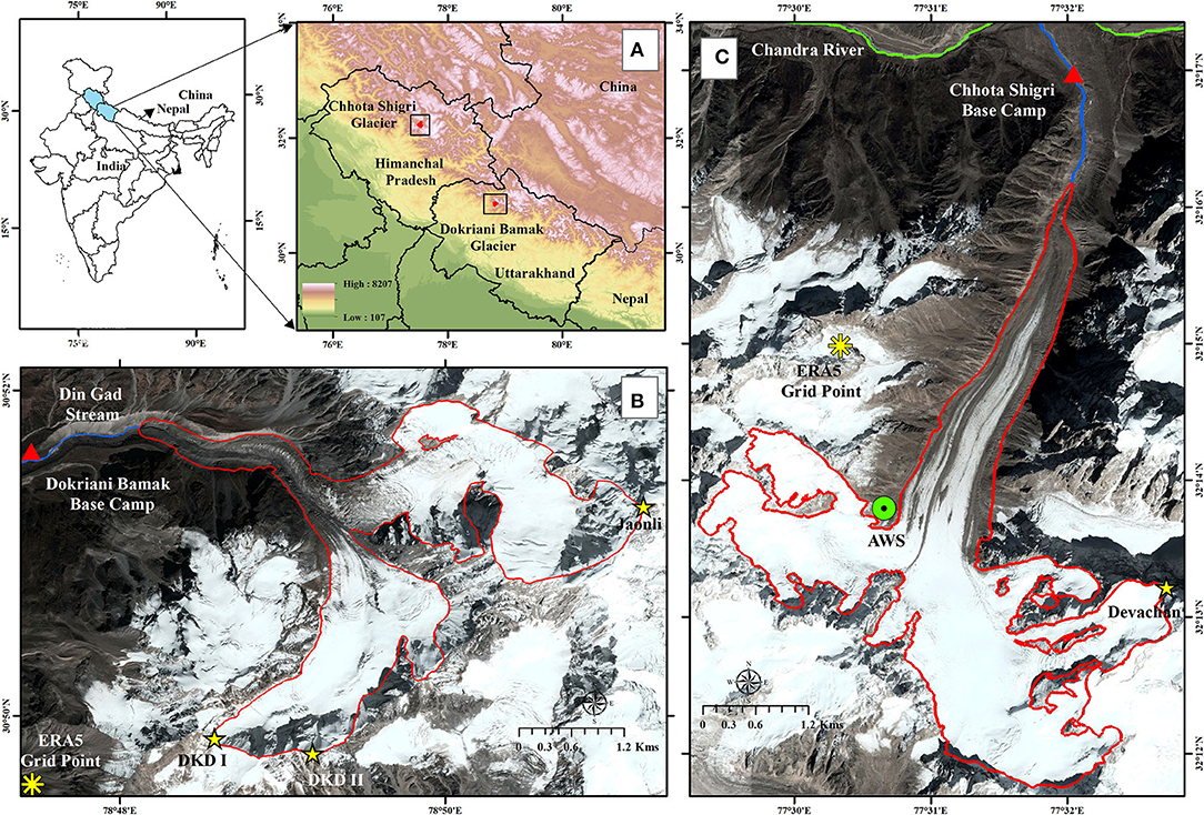
Figure 1. (A) The state boundary of Himanchal Pradesh and Uttarakhand along with locations of Dokriani Bamak and Chhota Shigri glaciers, (B) DBG (red outline) on Google earth imagery (CNES-Airbus) of 10 July 2017, and (C) CSG (red outline) on Google earth imagery (CNES-Airbus) of 10 April 2017.
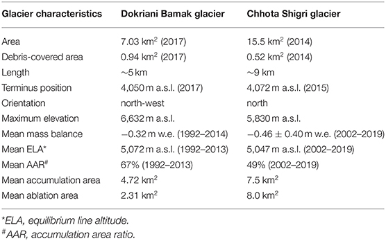
Table 1. List of geographical and topographical characteristics of DBG and CSG.
Chhota Shigri Glacier (32°16′ N, 77°34′ E) is in the Lahaul-Spiti valley of the western Himalaya (Figure 1). This is a valley glacier with a length of ~9 km and an area of 15.5 km2, and elevation ranging from 4,070 to 5,850 m a.s.l. (Table 1) (Azam et al., 2016). The CSG is a north-facing glacier, and its upper accumulation area is bounded by valley ridges, with Devachan Peak being the highest (6250 m a.s.l.) point. The terminus of CSG (<4,500 m a.s.l.) is covered with debris (~4% of CSG area) (Vincent et al., 2013). The CSG drains through a proglacial stream into the Chandra River, a tributary of the Indus River system (Figure 1). Since 2002, CSG is under continuous observations focusing on mass balances, SEB, ice thickness-volume-dynamics, and hydrology (Berthier et al., 2007; Wagnon et al., 2007; Soheb et al., 2017; Vashisht et al., 2017; Ramsankaran et al., 2018; Azam et al., 2019; Kumar et al., 2019; Mandal et al., 2020; Haq et al., 2021).
Available Field Data
DBG and CSG have extensively been studied; hence different datasets are available from previous studies. On DBG Base Camp (BC, 3,774 m a.s.l.), an automatic weather station (AWS) logged the data over 2011–2016 while on CSG an AWS, mounted on a side moraine close to high camp (HC, 4,863 m a.s.l.), provided the meteorological data between 2009 and 2017. An automated precipitation gauge (Geonor T-200B) at CSG BC (3,850 m a.s.l.) provided the data since 2012. Supplementary Table S2 provides the logging details of meteorological data. The locations of AWSs and all-weather precipitation gauge are given in Figure 1. The measurement of Ba on DBG were conducted intermittently during 1992–2014 (−0.32 m w.e. a−1; 1992–1995, 1996–2000, and 2007–2014) (Dobhal et al., 2021; Garg et al., 2021) while CSG represents the longest continuous Ba series since 2002 (−0.46 ± 0.40 m w.e. a−1) in the Himalaya (Mandal et al., 2020). Altitudinal mass balances (ba) are also available for 50-m bands over 2009–2013 for DBG (Pratap et al., 2015) and over 2002–2013 for CSG (Azam et al., 2016).
Climate Data and Bias Correction
Daily reanalysis data from ERA5 was used to compute the surface energy fluxes and glacier-wide mass balances on DBG and CSG. ERA5 data is available since 1979 at 0.25° × 0.25° resolution [Copernicus Climate Change Service (C3S), 2017]. The ERA5 data was found to be readily accessible, consistent, and available over a long period, and it has already been used for mass- and energy-balance models in a few studies (Kumar et al., 2021; Patel et al., 2021). Daily incoming shortwave and net radiation (SWI and SWN), incoming longwave radiation (LWI), wind speed (WS), relative humidity (RH), air temperature (Ta), and precipitation (P) were downloaded for the nearest grids at DBG and CSG (Figure 1). The ERA5 raw data series for both the glaciers were bias-corrected using available in-situ meteorological data (Supplementary Table S2). The bias correction of Ta was done using a linear regression between mean monthly and daily raw ERA5 and in-situ Ta data for DBG and CSG, respectively. The bias correction of daily P, WS, RH, SWI, SWN, and LWI were performed using monthly factors derived from monthly in-situ and ERA5 raw data on DBG and CSG. LWI in-situ data were available from DBG; hence no bias correction was given. All the bias-corrected parameters showed a good coefficient of determination after the bias correction (R2 > 0.90) (Supplementary Table S2). The details about the errors before and after bias correction and bias-correction factors are given in the Supplementary Material (Supplementary Figures S1–S13; Supplementary Table S3).
Methods
Mass- and Energy-Balance Model
The mass- and energy-balance model (Figure 2) computes the SEB fluxes and ba for each 50-m altitudinal range, and simulates snow accumulation, refreezing of rain/meltwater, surface melt, and sublimation/re-sublimation at daily time step using the long-term, bias-corrected daily ERA5 data between 1979 and 2020 (Section Study Area: Dokriani Bamak and Chhota Shigri Glaciers).
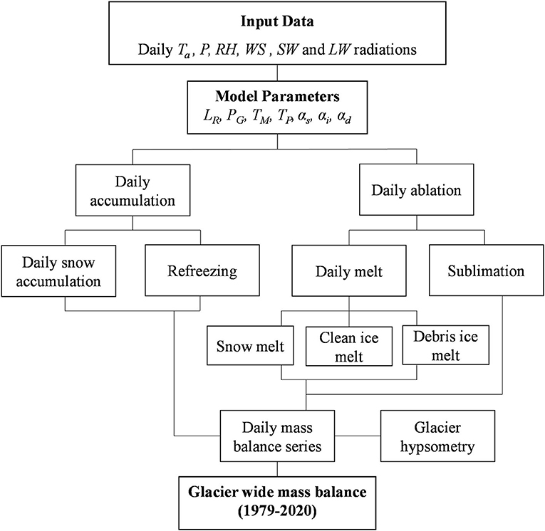
Figure 2. Mass- and energy-balance model structure. Ta is air temperature, P is precipitation, RH is relative humidity, WS is wind speed, SW and LW are the shortwave and longwave radiations, LR is the temperature lapse rate, PG is precipitation gradient, TM is threshold temperature for melt, TP is threshold temperature for precipitation, αs is the albedo of snow, αi is the albedo of ice, and αd is the albedo of debris cover.
Accumulation Terms
Accumulation terms include solid precipitation and refreezing of rain/melt water at the surface. At a given altitudinal range, the solid precipitation P (mm w.e. d−1) is computed as follows:
Where P and Ta represent daily precipitation (mm) and daily air temperature (°C), respectively, extrapolated at each 50-m altitudinal range, and TP represents the snow-rain threshold temperature (°C).
Refreezing of rain/melt water at each altitudinal range is computed using Oerlemans 2-m model (Oerlemans, 1992) in which the total energy available for melting (Qm) is determined by an exponential function of the temperature (θ) of the thermally active layer, considered equivalent to the upper 2-m thickness of a glacier:
Where, Q is the net surface energy budget (W m−2) and Hice is the heat flux generated by refreezing. At the beginning of the mass balance modeling, θ is set to the mean annual Ta, and can only be changed at the beginning of ablation season by refreezing the melt water derived from Equation 4. The value, c is a constant which determines how rapidly the melted snow or ice fraction that runs off reaches 1, and it was set to 1 K−1 (Oerlemans, 1992).
Sublimation/re-sublimation (Rs) is calculated using the latent heat flux (LE) (Equation 12) and the latent heat of vaporization (lv, 2.864 × 10⁶ J kg−1) is calculated as follows:
Ablation Terms
The major contribution to glacier ablation comes from the surface melt (Favier et al., 2004; Azam et al., 2014b; Litt et al., 2019) which is calculated using the net energy flux available at the surface. We used a simplified surface energy balance model:
Where αs, i, d is the albedo of snow (αs), ice (αi), and debris surface (αd), ε is the emissivity (dimensionless) considered 1, and σ is the Stefan Boltzmann constant = 5.67 × 10⁻⁸ W m−2 K−4, Ts is the surface temperature (°C). H, LE, and R are the turbulent sensible heat, latent heat, and rain fluxes (W m−2), respectively. Dynamic storage of snow over different altitudinal ranges was maintained using daily accumulation and ablation terms.
Computation of Surface Temperature
Surface temperature (TS) at each altitudinal range is computed following the calculation of Fujita and Ageta (2000):
Where, SWN is the net shortwave radiation (W m−2), le is the latent heat of evaporation of water (2.5 × 10⁶ J kg−1), ρa is the density of air (kg m−3), C is the bulk coefficient (0.002 for snow and clean ice and 0.005 for debris surfaces), q(Ta) is the saturated specific humidity, Hg is the heat transfer into the glacier (W m−2) (here, considered as zero), and ca is the specific heat of the air (1006 J kg−1 K−1). We have considered all the positive surface temperatures which are calculated from Equation 7 as zero because the glacier starts melting if Ta exceeds 0°C.
The value, ρa is estimated using the gas equation, where P is the air pressure (Pa) and Rspecific is the specific gas constant for dry air (287.058 J kg−1 K−1):
The values, q(Ta) and [q(Ts) in the next Section Computation of Turbulent Heat Fluxes], at a specific temperature, are calculated using the saturation vapor pressure (e*) at air and surface temperature, respectively and at air pressure (P) (k Pa):
Computation of Turbulent Heat Fluxes
The values of H, LE, and R are computed using the simplified bulk method (Hay and Fitzharris, 1988):
Where, cw is the specific heat of water (4,200 J kg−1 K−1), ρw is the density of water (kg m−3), Tr is the rainfall temperature (assumed equal to be Ta), w is the rainfall rate (m s−1), τw is the wetness parameter whose value is considered 1 for snow and ice surfaces, but it varies over the debris-covered surface (Supplementary Section 2). In the present study, we used the bulk method for the calculation of energy fluxes which is known to give reasonable results even in katabatic winds conditions (Denby and Greuell, 2000).
Computation of Mass Balance
The surface melt is calculated using the heat available for melting at different surfaces [Q(s, i, d), W m−2]. The net energy available at the surface is used to produce the melt when Ts is above the threshold temperature for melt (TM); otherwise, it is used to raise the Ts up to TM:
where lm is the latent heat of fusion (3.33 × 10⁵ J kg−1) and Q(s, i, d) is the amount of total energy available at the different surfaces.
The value, ba for each 50-m altitudinal range (m w.e.) is estimated using the accumulation and the ablation terms as follows:
Where ρw is the density of water (1,000 kg m−3).
Ba, (m w.e.) is calculated using the mean ba:
Where, Aa (m2) and ba (m w.e.) are the 50-m altitudinal glacier area and mean mass balance, respectively, and A is the total glacier area (m2). The value, Ba is calculated using daily values for the hydrological year from 1 November through 31 October of the next year for the DBG (Dobhal et al., 2008) and hydrological year from 1 October through 30 September of the next year for the CSG (Wagnon et al., 2007). The overall structure of the model is given in Figure 2.
Model Parameters
In the mass-, and energy-balance model, Ta is one of the most important parameters, as it decides the precipitation phase (snowfall or rain) (Hock, 2003; Shea et al., 2015a). In this study we calculated the extrapolated values of Ta using the temperature lapse rates (TLR) developed using field observations (Azam et al., 2014a; Azam and Srivastava, 2020). Further, the Tp values were adopted from Jennings et al. (2018), where we used a Tp value of 0.7° and 1.1°C corresponding to 70–80% and 60–70% RH ranges for DBG and CSG, respectively, at which 90–100% precipitation was considered as snow.
The net solar radiation is also crucial in the surface mass, and energy-balance modeling, and the amount of insolation available for melt production largely depends on surface albedo (Azam et al., 2014b; Litt et al., 2019). Surface albedo values (αs, αi, and αd) have high spatiotemporal variability over the glaciers. Deposition of dust and black carbon aerosols together with progressive snow metamorphism and compaction makes albedo values very uncertain (Oerlemans and Knap, 1998; Brock and Arnold, 2000). Moreover, the mass, and energy-balance models are highly sensitive to surface albedo (Kayastha et al., 1999; Acharya and Kayastha, 2019; Johnson and Rupper, 2020; Stigter et al., 2021); therefore, surface albedo values (αs, αi, αd) are calibrated in the present study using the plausible ranges available from the study of Cuffey and Paterson (2010). Due to lack of information related to surface albedo evolution in the study area as well as to keep the model computationally simple, we have used static but separate calibrated albedo values for snow, ice, and debris surfaces, as also adopted in some other previous studies (Ragettli et al., 2013, 2015; Acharya and Kayastha, 2019). Energy, and mass-balance models are also sensitive to TM, often unknown in the HK (Engelhardt et al., 2017; Azam et al., 2019; Azam and Srivastava, 2020). Further, the distribution of precipitation over glaciers is one of the biggest challenges in glaciological modeling, and it is spatially non-uniform in the HK region due to valley-specific precipitation gradients (PG) (Maussion et al., 2014; Immerzeel et al., 2015; Sakai et al., 2015). Given that TM, PG, αs, αi, and αd are highly sensitive parameters and least explored in the HK region; therefore, they are used for the calibration of the mass- and energy-balance model in this study.
Model Calibration
For the calibration of the mass- and energy-balance model, Monte Carlo simulations are performed with 10,000 parameter sets where the parameters are varied over their plausible limits (Konz and Seibert, 2010; Rounce et al., 2020). The value, PG is changed from 0 to 100% km−1, TM from −3°C to +3°C, αs from 0.45 to 0.85, αi from 0.35 to 0.55, and αdfrom 0.1 to 0.2 following the study by Cuffey and Paterson (2010). The runs with minimum RMSE between modeled and in-situ Ba are selected for both the glaciers. The selected runs show an RMSE of 0.21 m w.e. a−1 (1992–2014) and 0.32 m w.e. a−1 (2002–2019) between modeled and in-situ Ba for DBG and CSG, respectively. The difference between the modeled and in-situ mean Ba are 0.01 and 0.06 m w.e. a−1 on DBG and CSG, respectively (Table 2; Figure 3).
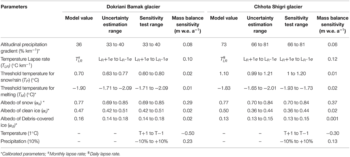
Table 2. List of model parameters, sensitivity and uncertainty ranges for DBG and CSG.
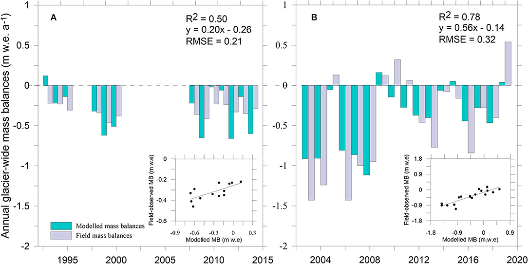
Figure 3. Model calibration: the modeled (green) and in-situ (violet) Ba on DBG over 1992-2014 (A), and CSG over 2003–2019 (B). Insets in both the panels show the correlations between modeled and in-situ mass balances.
Model Validation
Altitudinal Mass Balances
The model is validated against the in-situ mean ba available for 50-m bands from 4,050 to 4,950 m a.s.l. over 2009–2013 for DBG and from 4,250 to 5,300 m a.s.l. over 2002–2013 for CSG (Section Available Field Data). The agreement between modeled and in-situ ba shows a good agreement with R2 of 0.88 and 0.98 over clean ice on DBG and CSG, respectively (Figures 4A,B). Conversely but expectedly, this agreement over debris cover is very poor on both the glaciers. This is due to the strong spatial variability in debris distribution on both the glaciers that results in strong heterogeneous melt over the debris cover area (Vincent et al., 2013; Pratap et al., 2015). The in-situ ba at each altitudinal range were estimated by taking a single stake data or the mean of a couple of stakes inserted at selected flat locations having moderate (5–40 cm) debris thickness (avoiding very thick debris) on both the glaciers (Wagnon et al., 2007; Pratap et al., 2015); hence the estimated ba does not represent the whole 50-m altitudinal range. The debris-cover area (DBG = ~13%; CSG = ~4%) and the melt contribution (DBG = 17%; CSG = 6%) on both the glaciers is limited; therefore, the impact of possible mismatch between modeled and observed ba over debris cover on Ba can be assumed small. This assumption is also supported by the negligible modeled Ba sensitivity to αd on both the glaciers (Section Annual Glacier-Wide Mass Balance Sensitivity; Table 2). Though the comparison of modeled ba with in-situ data over debris cover serves no purpose, it echoes the limitation of conventional glaciological method for mass balance estimation over debris cover area (Azam et al., 2018).
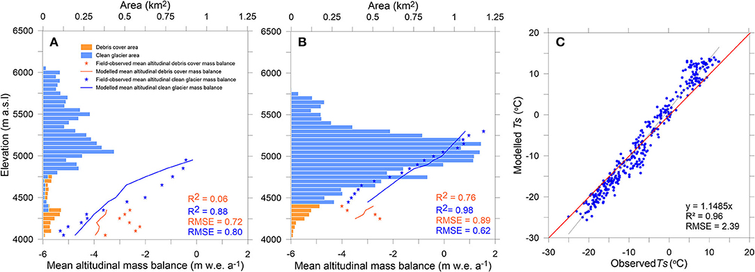
Figure 4. Model validation: the modeled and in-situ mean ba over 2009–2013 for DBG (A), over 2002–2013 for CSG (B), and surface temperature (C) [In (A,B), orange and blue bars show the 50-m hypsometry of debris-covered and clean glacier; orange and blue stars show the in-situ mean ba for the debris-covered and clean glacier; orange and blue lines show the modeled mean ba for the debris-covered and clean glacier].
Surface Temperature
Surface energy balance models are very sensitive to Ts; thus, another validation is performed for Ts. The modeled daily Ts (Section Computation of Surface Temperature) are compared with the observed Ts, derived from the bias-corrected LWO at CSG AWS. A good agreement between the modeled and observed Ts (R2 = 0.96; 14.85% overestimation, Figure 4C) indicates the robustness of the surface temperature scheme. The in-situ LWO data are not available for DBG; hence a similar validation could not be performed there. These validations of the model output against the observed ba (Figures 4A,B) and observed Ts (Figure 4C) suggest that the model is robust enough to reconstruct the mass balances.
Uncertainty Estimation
The model parameters are the key source of uncertainty in the modeled mass balances (Ragettli et al., 2013; Shea et al., 2015b). Parametric uncertainties are calculated by re-running the model while adjusting the parameters one-by-one within a reasonable range of their calibrated values and keeping the other model parameters unchanged (Table 2). The uncertainties in TLR are taken as standard deviations of mean monthly values for both DBG and CSG. The uncertainties in other parameters (αs, αi, αd, PG, TM and TP) are unknown; hence these parameters are varied with the range of ±10% from their calibrated values (Anslow et al., 2008; Ragettli et al., 2013, 2015).
The total uncertainty in Ba is calculated by summing up all parametric uncertainties by applying the error propagation rule. The estimated mean uncertainties for Ba are 0.32 m w.e a−1 and 0.38 m w.e a−1 for DBG and CSG, respectively over 1979–2020. Among all the parameters, the highest uncertainty in Ba on both the glaciers is contributed by αs (Table 2). The parametric uncertainty in the summer and winter mass balances are 0.38 and 0.01 m w.e a−1 for DBG and 0.36 and 0.02 m w.e. a−1 for CSG, respectively over 1979–2020.
In this study, a fixed glacier hypsometry was used on both the glaciers. For DBG, the hypsometry was manually delineated from high-resolution CNES-Airbus data from 10 July 2017 using a high-resolution Google Earth platform (Azam and Srivastava, 2020) while hypsometry for CSG was estimated using a digital elevation model (DEM) developed using Pléiades stereo pair from 18 August 2014 (Azam et al., 2016). This fixed area assumption introduces uncertainties to the modeled Ba, but these were found to be insignificant comparing the total estimated uncertainty in Ba in previous studies using T-index models (Azam et al., 2019; Azam and Srivastava, 2020), and hence they are ignored in this present study.
Results
Meteorological Conditions and Seasonal Characteristics
The HK Mountain range is located in the sub-tropical climate zone with a large annual temperature amplitude resulting in clear summer and winter seasons. The climate of HK is controlled by the Indian winter monsoon (IWM), embedding western disturbances, mainly during winters and the Indian summer monsoon (ISM), mainly during the summer (Gadgil et al., 2003; Dimri et al., 2016). The influence of IWM decreases eastwards; conversely, the intensity of the ISM decreases westwards along with the HK mountain range (Maussion et al., 2014). In-situ meteorological data from DBG and CSG are available for short periods (Section Available Field Data); therefore, long-term, bias-corrected ERA5 data over 1979–2020 are exploited to understand the mean seasonal characteristics on both the glaciers.
Mean monthly cycles of Ta and RH on both the glaciers followed roughly similar trends; however, the WS showed strong seasonality on DBG and moderate winds on CSG (Figure 5). The amplitudes of mean monthly Ta and RH (TaDBG = −7.2°C and RHDBG = 46% on DBG and TaCSG = −6.1°C and RHCSG = 47% on CSG) were sufficiently large to characterize the different seasons. A humid, warm, and less windy summer-monsoon from June through September and a less humid, cold, and windy winter season from December through March were demarcated on both the glaciers (Figure 5). A pre-monsoon over April–May and a post-monsoon over October–November were also defined (Supplementary Table S4). The same season demarcation was suggested on CSG by Azam et al. (2014a) using 3-years of AWS data (Figure 1).

Figure 5. Glacier-wide mean monthly values of Ta (red dots), Ts (brown dots), RH (green triangles), WS (blue circles), P (gray bars), SWI (orange bars) and LWI (violet bars) at (A) DBG base camp (3,774 m a.s.l.) and (B) CSG high camp (4,863 m a.s.l.), respectively from bias-corrected ERA5 data over 1979–2020. SWI and LWI are at point scale while all other parameters are at glacier-wide scale.
The summer-monsoon was the warmest (TaDBG = −1.5°C, TaCSG = 1.8°C), least windy (WSDG = 3.6 m s−1, WSCSG = 4.8 m s−1), and the most humid (RHDBG = 63%, RHCSG = 61%) season of both the glaciers (Supplementary Table S4). Conversely, the winter season was the coldest, much below the freezing point (TaDBG = −12.7°C, TaCSG = −13.5°C), and windiest (WSDBG = 8.8 m s−1, WSCSG = 5.7 m s−1) on both the glaciers. Pre-monsoon and post-monsoon showed the moderate conditions for Ta, RH, and WS (Supplementary Table S4). Modeled surface temperature (Ts) was always negative on both the glaciers except for the summer-monsoon when it was close to 0°C, showing the melting at the surface due to higher Ta of the summer monsoon (Supplementary Table S4).
The mean monthly P cycles were remarkably different on both the glaciers (Figure 5). The ISM brought the major amount of annual P (74%) over DBG during the summer monsoon, while IWM brought the major amount of annual P (53%) over CSG during the winter. Therefore, these glaciers can be considered as summer accumulation-type and winter accumulation-type glaciers, respectively. The mean annual P on DBG was almost double that of CSG (Supplementary Table S4). Systematically, P amounts on DBG in all seasons were 1.5–2 times less than that of CSG except the summer monsoon when P on DBG was 9 times compared to CSG (Supplementary Table S4).
Despite the maximum solar angle in the summer monsoon, SWI was maximum during pre-monsoon on both the glaciers (SWIDBG = 298 W m−2, SWICSG = 418 W m−2) because monsoonal cloud cover impedes the SWI in the summer monsoon (Azam et al., 2014b; Litt et al., 2019). However, this effect was much stronger on DBG due to strong monsoonal influence (Figure 5). The reduced SWI (SWIDBG = 294 W m−2, SWICSG = 410 W m−2) during the summer monsoon was compensated by the highest LWI (LWIDBG = 310 W m−2, LWICSG = 272 W m−2) on both the glaciers—mostly emitted from warm, dense summer-monsoonal clouds, and surrounding valley walls. Post-monsoon and winter exhibited quite similar conditions, receiving lower SWI and LWI due to decreasing solar angle, Ta, and RH (Supplementary Table S4).
Glacier-Wide Annual and Seasonal Mass Balances
The modeled mass wastage was moderate and similar on both the glaciers with a mean wastage of −0.27 ± 0.32 m w.e. a−1 (equivalent cumulative mass wastage of −11.16 ± 2.06 m w.e.) on DBG and −0.31 ± 0.38 m w.e. a−1 (equivalent cumulative mass wastage of −12.61 ± 2.67 m w.e.) on CSG, over 1979–2020 (Figure 6). The years 1982/83 and 1988/89 showed the maximum Ba of 0.20 ± 0.33 m w.e. and 0.42 ± 0.23 m w.e., while the year 2000/01 showed the minimum Ba of −0.75 ± 0.32 m w.e. and −1.49 ± 0.76 m w.e. for DBG and CSG, respectively. The value of Ba was negative for 35 and 27 years and positive for 6 and 14 years on DBG and CSG, respectively. Though the mean mass wastage on both the glaciers was almost the same, the mass turnover on CSG (1.27 m w.e. a−1) was higher than that of DBG (0.92 m w.e. a−1) (Figure 6). This is due to the fact that CSG is a winter accumulation-type glacier and receives a lot of accumulation during winter and is melted out during the summer-monsoon, while for DBG, the accumulation and ablation seasons coincide during the summer monsoon (Section Meteorological Conditions and Seasonal Characteristics).
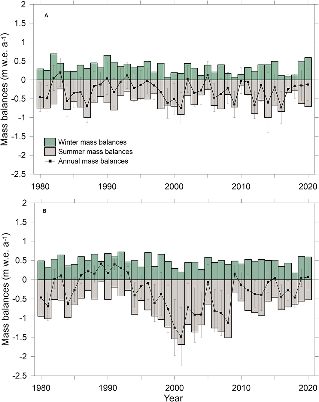
Figure 6. Annual mass balances (black squares), winter mass balances (green bars), and summer mass balances (gray bars) over 1979-2020 on (A) DBG and (B) CSG, respectively. The uncertainties of annual mass balances are shown.
Modeled seasonal mass balances ranged from 0.07 to 0.69 m w.e. a−1 and 0.17 to 0.72 m w.e. a−1 for winter, and −1.00 to −0.16 and −1.69 to −0.06 w.e. a−1 for summer on DBG and CSG, respectively. The mean summer and winter mass balances were −0.60 ± 0.30 and 0.32 ± 0.02 m w.e. a−1 on DBG and −0.79 ± 0.36 and 0.48 ± 0.02 m w.e. a−1 on CSG for the period 1979–2020, respectively.
Seasonal and Annual Glacier-Wide Surface Energy Balance
Surface energy balance mainly depends on the seasons (Litt et al., 2019). In the summer-monsoon, SWN was the highest with mean values of 100 and 125 W m−2 on DBG and CSG, respectively, with high daily variability from 71 to 151 W m−2 and 76 to 171 W m−2, respectively (Figure 7). The LWN was also maximum, with mean values of −4 and −41 W m−2 on DBG and CSG, respectively, in the summer monsoon due to humid, warm, and dense cloud cover conditions that result in high values of LWI (Supplementary Tables S4, S5). Highest SWN and LWN resulted in the highest net radiation (Rn) at the surface during the summer monsoon with the mean seasonal values of 95 and 84 W m−2 on DBG and CSG, respectively (Figure 7; Supplementary Table S5). Both the glaciers gained a small amount of energy through H. Conversely, a small amount of energy was released through LE—indicating some mass loss through sublimation (Supplementary Table S5). The resulting energy, Q, was the highest and positive during the summer monsoon on both the glaciers mainly due to the highest values of both SWN and LWN (Supplementary Table S5).
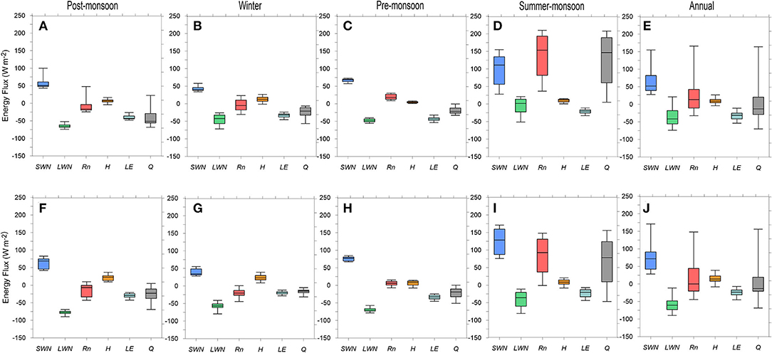
Figure 7. Box-whisker plots of mean daily SEB components calculated from all available data from 1979-2020 and classified into seasons, post-monsoon, winter, pre-monsoon, and summer-monsoon. The boundaries of each box cover the 25th to the 75th percentile of each distribution, while the middle line of the box shows the median value. Box-whisker in (A–E) shows the values for DBG and (F–J) CSG, respectively.
In winter, SWN was the least with 42 and 37 W m−2 values while LWN remained moderate with −45 and −57 W m−2 values on DBG and CSG, respectively (Supplementary Table S5). Winter SWN and LWN showed comparatively less variability on both the glaciers (Figure 7). In winter, DBG and CSG released some energy (−3 and −20 W m−2, respectively) through Rn (Figure 7). Like CSG, a recent study also found negative Rn during winter on 8 glaciers in the Chandra valley, including CSG (Patel et al., 2021). Due to the higher temperature gradient and strongest WS in winter (Supplementary Table S4), H was the maximum and provided 13 and 23 W m−2 energy at the surface of DBG and CSG, respectively (Supplementary Table S5). The LE was moderately negative during winter showing moderate glacier-wide sublimation (Supplementary Table S5). The net energy, Q, was also moderate but negative with −23 and −16 W m−2 values, mainly due to the least values of winter SWN on both the glaciers (Supplementary Table S5).
In pre-monsoon and post-monsoon, the SWN values were moderate as 67 and 56 W m−2 on DBG, and 87 and 61 W m−2 on CSG, respectively (Supplementary Table S5). Energy loss through LWN was the highest in post-monsoon when compared to other seasons on both the glaciers (Figure 7). The value Rn was positive in pre-monsoon while negative in post-monsoon (Supplementary Table S5) due to the most negative LWN values in post-monsoon on both the glaciers. Both DBG and CSG gained more energy in the form of H in post-monsoon than in pre-monsoon (Figure 7). The most negative values of LE in pre-monsoon and post-monsoon (Supplementary Table S5) indicate the maximum mass loss through sublimation during these seasons. The Q value was the least in both pre-monsoon and post-monsoon due to higher negative values of LWN and LE, and moderate values of SWN (Supplementary Table S5).
Similar to previous studies on the HK region (Mölg et al., 2012; Azam et al., 2014b; Huintjes et al., 2015a,b; Johnson and Rupper, 2020; Patel et al., 2021), annual glacier-wide SWN contributed the maximum amount of energy to the total SEB on DBG and CSG. Further, both the glaciers lost energy through LWN at −35 and −57 W m−2, respectively. The value of H brought some energy throughout the year with 9 and 15 W m−2 values on DBG and CSG, respectively (Supplementary Table S5; Figure 7). Patel et al. (2021) also observed a similar mean annual value of H on 8 glaciers in the Chandra valley (Figure 7). LE remained negative throughout the year on both the glaciers indicating mass loss through sublimation, in line with other glacier-wide SEB studies in the HK region (Huintjes et al., 2015a,b; Patel et al., 2021). Annually, the highest SWN results in maximum Rn followed by H and LE on both the glaciers. Annual glacier-wide net energy, Q, was positive with a value of 10 W m−2 on both DBG and CSG (Supplementary Table S5), indicating a net glacier-wide wastage (Section Glacier-Wide Annual and Seasonal Mass Balances).
Altitudinal Distribution of Mean Annual Mass Balance and SEB
The mean 50-m ba varied from −4.62 to 2.20 m w.e. on DBG and −1.95 to 0.57 m w.e on CSG (Figure 8). On DBG, the terminus area less than 4,950 m a.s.l. showed less glacier wastage toward the valley walls compared to the middle of the glacier (Figure 8). This is due to the distribution of debris cover on DBG which is thicker toward valley walls (Pratap et al., 2015). Similarly, the CSG terminus area less than 4,400 m a.s.l. also showed less mass wastage (Figure 8) due to thick debris cover (Vincent et al., 2013). Despite the lowest albedo of debris cover which results in the highest SWN over the debris-covered glacier with mean values of 188 and 141 W m−2 on DBG and CSG, respectively, the melting was the least due to a thick debris cover that protects the glacier from higher melt (Vincent et al., 2016; Banerjee, 2017). Going up on the glacier, the ba increased and becomes positive in the accumulation areas on both the glaciers (Figure 8). The increase in ba with altitude closely followed SWN which continuously reduced with altitude and achieved near-constant values of 56 and 59 W m−2 at higher altitudes on DBG (>5,250 m a.s.l.) and CSG (>5,050 m a.s.l.) glaciers, respectively. This was probably due to the permanent snow cover in the accumulation area, having higher surface albedo values near stable SWN. Glaciers lost some energy through LWN which was highly negative over lower reaches (<4,500 m a.s.l.) compared to higher altitudes on both the glaciers (Figure 8). The value of Rn was higher over lower reaches (<4,850 m a.s.l.), and showed a reduction between 4,800 to 5,500 m a.s.l. and again increased slightly toward higher reaches (>5,500 m a.s.l.) due to the highest LWN at higher reaches on both the glaciers (Figure 8). The DBG showed high and positive H values at lower altitudes (<5,250 m a.s.l.) and slightly negative values at higher altitudes due to the negative air-surface temperature gradient (Ta – Ts) while it remained positive over the whole CSG (Figure 8). The LE, generally more negative at higher altitudes, showed altitudinal mass loss through sublimation equivalent to −6 to −42 W m−2 on both DBG and CSG (Figure 8). The resulting energy, Q, was positive at lower altitudes (<5,000 m a.s.l.) and became negative at higher altitudes on both the glaciers (Figure 8).
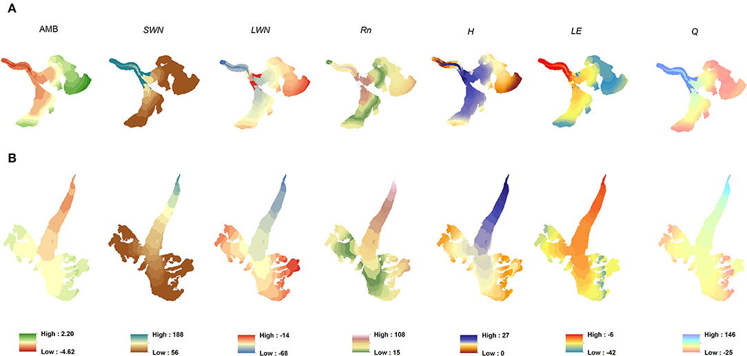
Figure 8. Distribution of modeled mean altitudinal mass balances and mean SEB components for 1979–2020 period of (A) DBG and (B) CSG, respectively (DBG and CSG are not in same scale).
On the DBG terminus area (<4,950 m a.s.l.), all the SEB components showed different behaviors toward valley walls as compared to the middle of the glacier due to the thick debris cover over the valley walls (Figure 8). Due to the low albedo of debris cover, SWN was the highest that resulted in maximum Rn and Q over those areas (Figure 8). H was slightly negative over debris-covered area compared to positive values at the middle of the glacier while LE was slightly less negative over the debris-covered area compared to more negative values at the middle of the glacier. This is due to the higher Ts than Ta over the debris-covered area due to the unavailability of snow or ice cover mainly during the summer-monsoon (Figure 8).
Glacier-Wide Sublimation
The mean glacier-wide sublimation was computed as −1.28 and −0.66 mm w.e. d−1 over 1979–2020, with a strong spatial and temporal variability, on DBG and CSG, respectively (Figures 8, 9). The mean monthly sublimation was higher in May on both DBG (−1.93 mm w.e. d−1) and CSG (−1.06 mm w.e. d−1) glaciers, and sharply decreased over July–August as soon as monsoon arrived over these glaciers (Figure 9). Despite the lowest WS, the highest RH and Ta in the summer-monsoon months (Figure 9) reversed the specific humidity gradient. This reversal led to slightly positive values of LE, at least over the ablation area, in July–August indicating re-sublimation on both the glaciers (Section SEB in Ablation and Accumulation Zones). This provided the least glacier-wide values of LE and the least amounts of sublimation in the summer-monsoon on both the glaciers (Figure 9). The sign reversal of LE from the negative to positive values during humid and warmer conditions has also been observed from SEB studies on different mountain ranges, including the HK region (Wagnon et al., 1999, 2003; Oerlemans, 2000; Sicart et al., 2005; Azam et al., 2014b; Stigter et al., 2018; Litt et al., 2019). Even though the WS was the highest in winter, the mean monthly glacier-wide sublimations were moderate due to the lowest RH and Ta on both the glaciers, whereas sublimation was the highest during pre-monsoon and post-monsoon months corresponding to moderate WS, RH, and Ta (Figure 9). The computed glacier-wide sublimation losses account for significant amounts of 22 and 20% of total ablation on DBG and CSG, respectively; therefore, we stress that the inclusion of a simplified sublimation scheme in mass balance modeling using T-index models, have not yet included. Simplified scheme may parametrize the sublimation as a function of temperature, humidity, and wind speed (Azam et al., 2021).
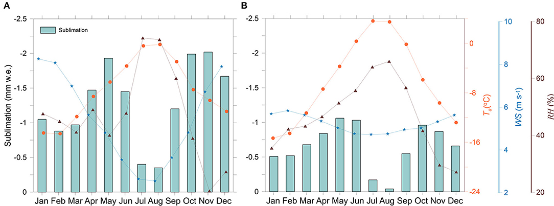
Figure 9. Monthly mean glacier-wide Ta (orange dots), RH (brown triangles), WS (blue stars), sublimation (blue-green bars) on (A) DBG and (B) CSG.
Relative Mass Wastage From Snow, Clean Ice, and Debris-Covered Ice
Snow, clean ice, and debris-covered ice ablation contributed 56, 27, and 17% to the total ablation on DBG, while on CSG, these contributions were 65, 29, and 6%, respectively. In agreement to the highest glacier-wide snow ablation over both the glaciers, previous glacio-hydrological T-index modeling studies also suggested that the snowmelt contribution was the maximum on DBG and CSG (Engelhardt et al., 2017; Azam et al., 2019; Azam and Srivastava, 2020). A slightly higher percentage of snow ablation on CSG compared to DBG is probably due to the reason that it gets around 53% of its annual precipitation in winter months that melt out in the summer-monsoon months while DBG receives 74% of its annual precipitation in the summer-monsoon when Ta is the highest which might result in rainfall on DBG even up to 5,100 m a.s.l. (Pratap et al., 2015) (Section Meteorological Conditions and Seasonal Characteristics). Under similar mass wastage conditions (Section Glacier-Wide Annual and Seasonal Mass Balances), the percent contribution of melt from debris-covered ice on DBG was three times of CSG due to three-folds of debris-covered ice on DBG (~13%) compared to CSG (~4%) (Vincent et al., 2013; Pratap et al., 2015).
Discussion
SEB in Ablation and Accumulation Zones
Most of the SEB studies in the HK have been performed at point-scale in the ablation zones (Azam et al., 2018; Litt et al., 2019). However, a few glacier-wide studies suggested that SEB is quite different in the ablation and accumulation zones of glaciers (Sun et al., 2014; Patel et al., 2021). To investigate the SEB in the ablation and accumulation zones of DBG and CSG, we estimated the mean annual ablation-wide and accumulation-wide SEBs separately, dividing the ablation and accumulation zones using the mean ELA from the literature (Table 1).
Mean monthly SWN budgets were similar over the ablation zones of both the glaciers: strong mean monthly cycles had the highest SWN in August during the summer monsoon and the lowest SWN in the winter, while relatively moderate values in the accumulation zone throughout the year except the winter when SWN were the lowest on both the glaciers (Supplementary Table S6; Figure 10). In winter, both the glaciers were completely covered by snow which resulted in higher surface albedo and similar ablation- and accumulation-wide SWN budgets (Supplementary Table S6). Negative LWN budgets showed higher loss of energy in the ablation zone compared to the accumulation zone throughout the year with most negative values in winter on both the glaciers (Supplementary Table S6; Figure 10), except slightly positive values in July–August on DBG most probably due to the highest LWI of heavy monsoonal cloud cover (Supplementary Table S4). Mean monthly H were positive as Ta was higher than Ts in the ablation zones of both the glaciers, while negative in the accumulation zones during the summer monsoon and pre-monsoon (Supplementary Table S6; Figure 10) as Ts becomes higher than Ta on both the glaciers (Supplementary Table S4). The LE was consistently negative in the accumulation zones of both the glaciers suggesting continuous mass loss through sublimation from higher altitudes; however it was slightly positive in the ablation zones over July–August on both the glaciers indicating re-sublimation during the core summer-monsoon (Figure 10). The resublimation was 3.50 and 2.04% on DBG and CSG respectively, compared to sublimation in the ablation zone. The value, Q remained negative throughout the year except for the summer monsoon in the ablation zones and July–August in the accumulation zones due to higher SWN on both the glaciers. Similar results have been discussed in other SEB studies on the Himalayan glaciers (Azam et al., 2014b; Litt et al., 2019; Patel et al., 2021).

Figure 10. SEB in ablation and accumulation zones of (A) DBG and (B) CSG.
Major Drivers for Glacier Mass Balances
Due to the scarcity of mass balance and meteorological data in the HK, the climatic drivers controlling the mass balances have been poorly discussed (Azam et al., 2014a, 2018; Shea et al., 2015a). To comprehend the major drivers controlling the glacier-wide seasonal and annual mass balances, the correlation coefficients (r) were developed amid annual and seasonal mass balances, bias-corrected mean annual ERA5 data, and surface energy fluxes over 1979–2020 on both the glaciers (Figure 11).

Figure 11. (A,B) A graphical representation of correlations with 1% (0.01) p significance values among the inter-annual variability of mass balance, energy fluxes and its meteorological drivers during 1979–2020 for DBG and CSG, respectively (red color shows negative while blue color shows positive correlation values). WMB and SMB are winter and summer mass balances.
The value of Ba on DBG showed strong positive correlations (r = ~0.40–0.70) with P and surface albedo while moderately negative correlations (r = ~0.40–0.60) with SWN, Rn, and Q (Figure 11). Similarly, CSG also showed good correlations with P and surface albedo; however, the negative correlations with SWN, Rn and Q were stronger (r = ~0.80) (Figure 11). Due to their undersized role in total SEB (Section Seasonal and Annual Glacier-Wide Surface Energy Balance), H, LE, and LWN showed insignificant correlations with annual as well as seasonal mass balances on both the glaciers (Figure 11).
The value of Ba and summer mass balances on CSG showed moderate correlations with SWI while these correlations on DBG were insignificant (Figure 11). This is probably due to heavy monsoonal clouds that reduce the amount of SWI on DBG, resulting in low mean annual values (Supplementary Table S4). Winter mass balances on DBG showed weak positive correlation (r = 0.27) with P while a stronger positive correlation (r = 0.63) was observed on CSG (Figure 11). This is expected as DBG and CSG are summer and winter accumulation-type glaciers, respectively (Section Meteorological Conditions and Seasonal Characteristics). Further, summer mass balances on both the glaciers showed moderately positive but almost similar correlations (r = ~0.60) with P (Figure 11). Despite the fact that CSG receives its major annual precipitation during winter, almost similar correlation between summer mass balances and P occurs most probably due to sporadic summer-monsoonal snowfall events on CSG (Azam et al., 2019). A previous study on CSG investigated the critical role of summer-monsoon snowfalls in detail and concluded that these snowfalls often cover the whole or part of the ablation zone during peak melting months and abruptly reduce the SWI absorption and control the summer mass balances which further control the Ba (Azam et al., 2014b). The value of Ta showed weak and moderate negative correlations with Ba (r = −0.30) and summer (r = −0.52) mass balances, respectively on DBG, while showed moderate negative correlations with Ba (r = −0.44) and summer (r =-0.40) mass balances (Figure 11). The value of Ta was poorly correlated with winter mass balances on both the glaciers (Figure 11). However, as expected, Ta showed very strong correlations with Ts and LWO on both the glaciers (Figure 11).
The value of Ba on DBG and CSG showed moderately strong correlations with winter mass balances (r = 0.58 and r = 0.67, respectively) while showing very strong correlations with summer mass balances (r = 0.80, r = 0.97, respectively) (Figure 11). Higher dependency of Ba on summer mass balances suggests that both the glaciers have high vulnerability to regional warming; hence, expected to lose more mass in the continuation of warming (Banerjee and Azam, 2016; Kraaijenbrink et al., 2017; Krishnan et al., 2019; Mahto and Mishra, 2019).
Annual Glacier-Wide Mass Balance Sensitivity
Mass balance sensitivities were computed to understand the response of the glaciers to the changes in different model input parameters. These sensitivities were computed, one-by-one, by re-running the model with a unique set of each model parameter where hH was the highest and hL was the lowest value of parameter h, holding all the other parameters constant. Following Ragettli et al. (2013), the hH and hL were estimated by varying each parameter h by ±10% from its calibrated value except for Tm, Tp, Ta which were varied by 0.1, 0.1, and 1.0°C, respectively (Table 2). The mass balance sensitivities were estimated for the period 1979–2020 following (Oerlemans et al., 1998):
Where, Ba is the glacier-wide mass balance averaged over the period 1979–2020.
The estimated Ba sensitivities on DBG and CSG are given in Table 2. The Ba was the most sensitive to αs, with the sensitivities of 0.29 and 0.37 m w.e. a−1 on DBG and CSG, respectively (Table 2). Previous studies on other glaciers in the Alps and Himalaya also showed the maximum sensitivity of Bato αs (Klok and Oerlemans, 2004; Johnson and Rupper, 2020; Stigter et al., 2021). The modeled Ba showed moderate sensitivities to TLR (DBG = 0.10 m w.e. a−1; CSG = 0.12 m w.e. a−1). Sensitivities were quite low to Tp, TM, αd, αi and PG for both the glaciers (Table 2).
The sensitivity of the modeled mean Ba to 1°C change in Ta was higher on DBG (−0.50 m w.e. a−1) than CSG (−0.30 m w.e. a−1) whereas the sensitivities to 10% change in P were roughly the same (DBG = 0.23 m w.e. a−1, CSG = 0.13 m w.e. a−1) (Table 2). Higher sensitivity to Ta on DBG is probably due to different precipitation regimes on both the glaciers. DBG receives its maximum of annual precipitation in the summer monsoon when Ta is the highest; hence, DBG had more sensitivity to Ta compared to CSG that receives its major precipitation in winters (Fujita, 2008; Azam et al., 2014a). Using a T-index model, a previous study on CSG computed higher sensitivity (−0.52 m w.e. a−1) of mass balance to 1°C change in Ta and roughly similar sensitivity (0.16 m w.e. a−1) to 10% change in P (Azam et al., 2014a). Another study on Zhadang Glacier in Tibet showed similar results using an energy balance model with the sensitivity of −0.47 m w.e. a−1 to 1°C change in Ta and sensitivity of 0.14 m w.e. a−1 to 10% change in P (Mölg et al., 2012). Our sensitivity results are quite comparable with these studies in the mountain glaciers.
Comparison of Sublimation Rates With HK Glaciers
In this section, we discuss the sublimation rates from different studies on HK glaciers. However, irrespective of our glacier-wide and round-the-year study, often the studies were (i) available at point-scale, (ii) from different months of the year, (iii) having different locations of automatic weather stations (on/off glacier), and (iv) installed on different surfaces (snow and ice) that hinders a direct comparison. In the present study, the mean glacier-wide sublimation was computed as −1.28 and −0.66 mm w.e. d−1 over 1979–2020 on DBG and CSG, respectively. Previously, using in-situ AWS data from the middle of the ablation zone (4,670 m a.s.l.) on CSG, a point-scale SEB study computed a mean sublimation of −0.63 mm w.e. d−1 over 2012–2013 (Azam et al., 2014a). Another recent point-scale SEB study on seasonal snow surface on a lateral moraine of CSG only (4,863 m a.s.l.) suggested that sublimation was −1.1 mm d−1 during winters over 2009–2020 (Mandal et al., 2022). The mean glacier-wide sublimation was reported as −1.08 and −0.70 mm w.e. d−1 on Zhadang Glacier (south-central Tibetan Plateau) and on Puruogangri ice (north-central Tibetan Plateau) between 2001 and 2011 (Huintjes et al., 2015a,b). In the central Himalaya, the sublimation rate was reported for short-term snow-cover at the Pindari Glacier AWS site (off-glacier; 3750 m a.s.l.) to be −0.3 mm d−1 during winters (Singh et al., 2020). In the Nepal Himalaya, on Yala Glacier (5350 m a.s.l.) around −1.00 mm d−1 mass was lost through sublimation during winters (Stigter et al., 2018). In line, another study showed significant sublimation rate of −7.1 and −1.9 mm d−1 on Mera Glacier and −2.4 and −1.8 mm d−1 on Yala Glacier during the post- and pre-monsoon season, respectively (Litt et al., 2019).
Mass Balance Comparison With Other Studies
The in-situ glaciological method showed a mass wastage of −0.32 m w.e. a−1 on DBG over 1992–1995, 1997–2000, and 2007–2013 (Dobhal et al., 2021), while our model showed slightly lesser mass wastage of −0.27 ± 0.31 m w.e. a−1 over the same years (Figure 12A). On CSG, the glaciological method showed a mass wastage of −0.43 ± 0.40 m w.e. a−1 over 2002–2019 (Mandal et al., 2020), while our model showed similar mass wastage of −0.42 ± 0.42 m w.e. a−1 (Figure 12B).

Figure 12. Mass balance estimates on DBG (A) and CSG (B) glaciers from available studies.
Geodetic mass balances are also available on both the glaciers and are used here to validate the modeled mass-balance series. A recent study using high-resolution Cartosat-1 DEM and SRTM DEM estimated a mass wastage of −0.23 ± 0.10 m w.e. a−1 on DBG over 1999–2014 (Garg et al., 2021). Over the same period, our model showed slightly higher mass wastage with a mean mass balance of −0.35 ± 0.41 m w.e. a−1 on DBG. On CSG, our model showed higher mass wastage of −0.39 ± 0.43 m w.e. a−1 against a mass wastage of −0.27 ± 0.13 m w.e. a−1 over 2005–2014 derived using ASTER DEMs (Brun et al., 2017). Another geodetic study provided a mean mass wastage of −0.46 ± 0.34 m w.e. a−1 over 2000–2012 (Vijay and Braun, 2016), while our model computed a mean mass wastage of −0.67 ± 0.54 m w.e. a−1 over the same period. Another geodetic study combining SRTM and SPOT5 DEMs provided a mean mass wastage of −1.12 m w.e. a−1 using density assumption 1 and −1.02 m w.e. a−1 using density assumption 2 which is in close agreement with our model value (−1.01 m w.e. a−1) over 1999–2004 (Berthier et al., 2007) (Figures 12A,B).
Our modeled mean mass balance of −0.27 ± 0.39 m w.e. a−1 on DBG and −0.31 ± 0.38 m w.e. a−1 on CSG were in better agreement with the modeled mean mass balance of −0.25 ± 0.37 m w.e. a−1 and −0.26 ± 0.29 m w.e. a−1 from a simplified T-index model over 1979–2020 (Srivastava et al., 2021). The present study, showing a moderate mean mass balance on both the glaciers over 1979–2020, is in close agreement with most of the previous studies and nicely captures the inter-annual variability with other modeled MBs (Figures 12A,B).
Conclusion
Due to harsh climatic conditions, long-term in-situ glacio-meteorological observations are sparse in the HK region, which impedes an in-depth understanding of the glacier–climate relationship. A mass- and energy-balance model is used to get around this constraint, using the long-term ERA5 reanalysis data since 1979, for two climatically diverse glaciers of DBG and CSG where a fairly good amount of in-situ glacio-meteorological data are available from previous studies. The in-situ measurements are used to calibrate/validate the model for DBG and CSG. The model is further used to study the altitudinal patterns of mass balance and surface energy fluxes over both the glaciers.
Both the glaciers experience a warm and moist weather condition with low wind velocity during the summer monsoon (June–September) and a cold, dry windy condition during winter (December to March). Intermediate weather conditions persist during pre-monsoon (April to May) and post-monsoon (October-November). DBG receives the majority of precipitation (~74%) in the summer monsoon whereas CSG receives maximum precipitation (~53%) in winter.
DBG and CSG are losing mass at a moderate rate with the mean Ba of −0.27 ± 0.32 m w.e. a−1 and −0.31 ± 0.38 m w.e. a−1, respectively, over 1979–2020. Though the mean mass wastage on both the glaciers is similar, the annual mass turnover on CSG is higher than that on DBG. The mean summer and winter mass balances are computed to be −0.60 ± 0.30 and 0.32 ± 0.02 m w.e. a−1 on DBG and −0.79 ± 0.36 and 0.48 ± 0.02 m w.e. a−1 on CSG, respectively.
Glacier-wide net shortwave radiation has the dominant control over energy balance followed by longwave net radiation, latent heat flux, and sensible heat flux on both the glaciers. On the annual scale, both DBG and CSG showed a positive glacier-wide net energy of 10 W m−2 indicating a mass wastage over 1979–2020. Latent heat flux is always negative suggesting glacier-wide sublimation throughout the year except for peak summer monsoon when it is slightly positive over ablation zone indicating re-sublimation on both the glaciers. The losses through sublimation are around 22 and 20% of total ablation on DBG and CSG, respectively, with a strong spatial and temporal variability.
The value of Ba on DBG and CSG showed moderately strong correlations with winter mass balances, while showing very strong correlations with summer-mass balances, suggesting summer as the main mass balance driver season. The sensitivity of modeled mean Ba to 1°C change in Ta is higher on DBG (−0.50 m w.e. a−1) than the CSG (−0.30 m w.e. a−1) whereas the sensitivities to 10% change in P are nearly the same (DBG = 0.23 m w.e. a−1, CSG = 0.13 m w.e. a−1) over 1979–2020. Mass- and energy-balance model is the most sensitive to snow albedo followed by temperature lapse rates and least sensitivity to the rest of the model parameters on both the glaciers.
The modeled Ba on both the glaciers show a good agreement with the available mass balances from geodetic, model, and in-situ measurements. This study provides insights into the regional variations in mass-wastage governing SEB fluxes at glacier-wide scale, which is helpful for understanding the glacier–climate interactions in the Himalaya and stresses an inclusion of a sublimation scheme in T-index models. A possible, rapid advancement could be to assimilate the simplified scheme of sublimation, such as the empirical equation in T-index models of Kuchment and Gelfan (1996). However, such equations need to be tested for their transferability from one region to other.
Data Availability Statement
The original contributions presented in the study are included in the article/Supplementary Material, further inquiries can be directed to the corresponding author/s.
Author Contributions
MFA designed the study. SS developed the model and figures. SS and MFA did the analysis and wrote the paper. All authors contributed to the article and approved the submitted version.
Funding
SS acknowledges the research fellowship from the Space Application Centre (ISRO) through the Cryospheric Science and Application Program. MFA acknowledges the research grant from INSPIRE Scheme (IFA-14-EAS-22), from the Department of Science and Technology (DST, India), and the Core Research Grant (CRG/2020/004877) from Science and Engineering Research Board (SERB), DST, India.
Conflict of Interest
The authors declare that the research was conducted in the absence of any commercial or financial relationships that could be construed as a potential conflict of interest.
Publisher's Note
All claims expressed in this article are solely those of the authors and do not necessarily represent those of their affiliated organizations, or those of the publisher, the editors and the reviewers. Any product that may be evaluated in this article, or claim that may be made by its manufacturer, is not guaranteed or endorsed by the publisher.
Acknowledgments
The authors acknowledge the European Centre for Medium-Range Weather Forecasts (ECMWF) for keeping the data publicly accessible. The authors also thank the scientists who have collected the in-situ data on both the glaciers. A special thanks to Dr. Rajdeep for the stylistic improvement of the manuscript.
Supplementary Material
The Supplementary Material for this article can be found online at: https://www.frontiersin.org/articles/10.3389/frwa.2022.874240/full#supplementary-material
References
Acharya, A., and Kayastha, R. B. (2019). Mass and energy balance estimation of Yala glacier (2011–2017), Langtang valley, Nepal. Water 11, 6. doi: 10.3390/w11010006
Anslow, F. S., Hostetler, S., Bidlake, W. R., and Clark, P. U. (2008). Distributed energy balance modeling of South Cascade Glacier, Washington and assessment of model uncertainty. J. Geophys. Res. Earth Surf. 113, F2. doi: 10.1029/2007JF000850
Azam, M. F. (2021). Need of integrated monitoring on reference glacier catchments for future water security in Himalaya. Water Secur. 14, 100098. doi: 10.1016/j.wasec.2021.100098
Azam, M. F., Kargel, J. S., Shea, J. M., Nepal, S., Haritashya, U. K., Srivastava, S., et al. (2021). Glaciohydrology of the himalaya-karakoram. Science 373, eabf3668. doi: 10.1126/science.abf3668
Azam, M. F., Ramanathan, A. L., Wagnon, P., Vincent, C., Linda, A., Berthier, E., et al. (2016). Meteorological conditions, seasonal and annual mass balances of Chhota Shigri Glacier, western Himalaya, India. Ann. Glaciol. 57, 328–338. doi: 10.3189/2016AoG71A570
Azam, M. F., and Srivastava, S. (2020). Mass balance and runoff modelling of partially debris-covered Dokriani Glacier in monsoon-dominated Himalaya using ERA5 data since 1979. J. Hydrol. 590, 125432. doi: 10.1016/j.jhydrol.2020.125432
Azam, M. F., Wagnon, P., Berthier, E., Vincent, C., Fujita, K., and Kargel, J. S. (2018). Review of the status and mass changes of Himalayan-Karakoram glaciers. J. Glaciol. 64, 61–74. doi: 10.1017/jog.2017.86
Azam, M. F., Wagnon, P., Vincent, C., Ramanathan, A., Linda, A., and Singh, V. B. (2014a). Reconstruction of the annual mass balance of Chhota Shigri glacier, Western Himalaya, India, since 1969. Ann. Glaciol. 55, 6980. doi: 10.3189/2014AoG66A104
Azam, M. F., Wagnon, P., Vincent, C., Ramanathan, A. L., Favier, V., Mandal, A., et al. (2014b). Processes governing the mass balance of Chhota Shigri Glacier (western Himalaya, India) assessed by point-scale surface energy balance measurements. Cryosphere 8, 2195–2217. doi: 10.5194/tc-8-2195-2014
Azam, M. F., Wagnon, P., Vincent, C., Ramanathan, A. L., Kumar, N., Srivastava, S., et al. (2019). Snow and ice melt contributions in a highly glacierized catchment of Chhota Shigri Glacier (India) over the last five decades. J. Hydrol. 574, 760–773. doi: 10.1016/j.jhydrol.2019.04.075
Banerjee, A. (2017). Brief communication: Thinning of debris-covered and debris-free glacier in a warming climate. Cryosphere 11, 133–138. doi: 10.5194/tc-11-133-2017
Banerjee, A., and Azam, M. F. (2016). Temperature reconstruction from glacier length fluctuations in the Himalaya. Ann. Glaciol. 57, 189–198. doi: 10.3189/2016AoG71A047
Berthier, E., Arnaud, Y., Kumar, R., Ahmad, S., Wagnon, P., and Chevallier, P. (2007). Remote Sens. estimates of glacier mass balances in the Himachal Pradesh (Western Himalaya, India). Remote Sens. Environ. 108, 327–338. doi: 10.1016/j.rse.2006.11.017
Berthier, E., and Brun, F. (2019). Karakoram geodetic glacier mass balances between 2008 and 2016: persistence of the anomaly and influence of a large rock avalanche on Siachen Glacier. J. Glaciol. 65, 494–507. doi: 10.1017/jog.2019.32
Bolch, T., Pieczonka, T., Mukherjee, K., and Shea, J. (2017). Brief communication: glaciers in the Hunza catchment (Karakoram) have been nearly in balance since the 1970s. Cryosphere 11, 531–539. doi: 10.5194/tc-11-531-2017
Bolch, T., Shea, J. M., Liu, S., Azam, F. M., Gao, Y., Gruber, S., et al. (2019). Status and change of Cryosphere in the extended Hindu Kush Himalaya region, in The Hindu Kush Himalaya Assessment (Cham: Springer), 209–255
Brock, B. W., and Arnold, N. S. (2000). A spreadsheet-based (Microsoft Excel) point surface energy balance model for glacier and snow melt studies. Earth Surf. Process. Landf. 25, 649–658. doi: 10.1002/1096-9837(200006)25:6<649::AID-ESP97>3.0.CO;2-U
Brun, F., Berthier, E., Wagnon, P., Kääb, A., and Treichler, D. (2017). A spatially resolved estimate of High Mountain Asia glacier mass balances from 2000 to 2016. Nat. Geosci. 10, 668–673. doi: 10.1038/ngeo2999
Brun, F., Dumont, M., Wagnon, P., Berthier, E., Azam, M. F., Shea, J. M., et al. (2015). Seasonal changes in surface albedo of Himalayan glaciers from MODIS data and links with the annual mass balance. Cryosphere 9, 341–355. doi: 10.5194/tc-9-341-2015
Copernicus Climate Change Service (C3S) (2017). ERA5. Available online at: https://cds.climate.copernicus.eu/cdsapp#!/home (accessed April 6, 2022).
de Kok, R. J., Tuinenburg, O. A., Bonekamp, P. N., and Immerzeel, W. W. (2018). Irrigation as a potential driver for anomalous glacier behavior in High Mountain Asia. Geophys. Res. Lett. 45, 2047–2054. doi: 10.1002/2017GL076158
Denby, B., and Greuell, W. (2000). The use of bulk and profile methods for determining surface heat fluxes in the presence of glacier winds. J. Glaciol. 46, 445–452. doi: 10.3189/172756500781833124
Dimri, A. P., Yasunari, T., Kotlia, B. S., Mohanty, U. C., and Sikka, D. R. (2016). Indian winter monsoon: present and past. Earth-Sci. Rev. 163, 297–322. doi: 10.1016/j.earscirev.2016.10.008
Dobhal, D. P., Gergan, J. T., and Thayyen, R. J. (2008). Mass balance studies of the Dokriani Glacier from to, Garhwal Himalaya, India. Bull. Glaciol. Res. 25, 9–17.
Dobhal, D. P., Pratap, B., Bhambri, R., and Mehta, M. (2021). Mass balance and morphological changes of Dokriani Glacier (1992–2013), Garhwal Himalaya, India. Quat. Sci. Adv. 4, 100033. doi: 10.1016/j.qsa.2021.100033
Engelhardt, M., Ramanathan, A. L., Eidhammer, T., Kumar, P., Landgren, O., Mandal, A., et al. (2017). Modelling 60 years of glacier mass balance and runoff for Chhota Shigri Glacier, Western Himalaya, Northern India. J. Glaciol. 63, 618–628. doi: 10.1017/jog.2017.29
Farinotti, D., Immerzeel, W. W., De Kok, R. J., Quincey, D. J., and Dehecq, A. (2020). Manifestations and mechanisms of the Karakoram glacier. Anomaly Nat. Geosci. 13, 8–16. doi: 10.1038/s41561-019-0513-5
Favier, V., Wagnon, P., Chazarin, J. P., Maisincho, L., and Coudrain, A. (2004). One-year measurements of surface heat budget on the ablation zone of Antizana Glacier 15, Ecuadorian Andes. J. Geophys. Res. Atmos. 109, D18. doi: 10.1029/2003JD004359
Fujita, K. (2008). Effect of precipitation seasonality on climatic sensitivity of glacier mass balance. Earth Planet. Sci. Lett. 276, 14–19. doi: 10.1016/j.epsl.2008.08.028
Fujita, K., and Ageta, Y. (2000). Effect of summer accumulation on glacier mass balance on the Tibetan Plateau revealed by mass-balance model. J. Glaciol. 46, 244–252. doi: 10.3189/172756500781832945
Fujita, K., and Sakai, A. (2014). Modelling runoff from a Himalayan debris-covered glacier. Hydrol. Earth Syst. Sci. 18, 2679–2694. doi: 10.5194/hess-18-2679-2014
Fujita, K., Takeuchi, N., Nikitin, S. A., Surazakov, A. B., Okamoto, S., Aizen, V. B., et al. (2011). Favorable climatic regime for maintaining the present-day geometry of the Gregoriev Glacier, Inner Tien Shan. Cryosphere 5, 539–549. doi: 10.5194/tc-5-539-2011
Gadgil, S., Vinayachandran, P. N., and Francis, P. A. (2003). Droughts of the Indian summer monsoon: role of clouds over the Indian Ocean. Curr. Sci. 85, 1713–9. Available online at: https://www.jstor.org/stable/24109976
Gardelle, J., Berthier, E., and Arnaud, Y. (2012). Slight mass gain of Karakoram glaciers in the early twenty-first century. Nat. Geosci. 5, 322–325. doi: 10.1038/ngeo1450
Garg, P. K., Yadav, J. S., Rai, S. K., and Shukla, A. (2021). Mass balance and morphological evolution of the Dokriani Glacier, central Himalaya, India during 1999–2014. Geosci. Front. 13, 101290. doi: 10.1016/j.gsf.2021.101290
Haq, M. A., Azam, M. F., and Vincent, C. (2021). Efficiency of artificial neural networks for glacier ice-thickness estimation: a case study in western Himalaya, India. J. Glaciol. 264, 1–14. doi: 10.1017/jog.2021.19
Hay, J. E., and Fitzharris, B. B. (1988). A comparison of the energy-balance and bulk-aerodynamic approaches for estimating glacier melt. J. Glaciol. 34, 145–153. doi: 10.1017/S0022143000032172
Hewitt, K. (2005). The Karakoram anomaly? Glacier expansion and the ‘elevation effect,'Karakoram Himalaya. Mt. Res. Dev. 25, 332–340. doi: 10.1659/0276-4741(2005)0250332:TKAGEA2.0.CO;2
Hock, R. (2003). Temperature index melt modelling in mountain areas. J. Hydrol. 282, 104–115. doi: 10.1016/S0022-1694(03)00257-9
Hock, R., Rasul, G., Adler, C., Cáceres, B., Gruber, S., Hirabayashi, Y., et al. (2019). High mountain areas, in IPCC Special Report on Ocean and the Cryosphere in a Changing Climate (Geneva: IPCC).
Huintjes, E., Neckel, N., Hochschild, V., and Schneider, C. (2015a). Surface energy and mass balance at Purogangri ice cap, central Tibetan Plateau, 2001–2011. J. Glaciol. 61, 1048–1060. doi: 10.3189/2015JoG15J056
Huintjes, E., Sauter, T., Schröter, B., Maussion, F., Yang, W., Kropáček, J., et al. (2015b). Evaluation of a coupled snow and energy balance model for Zhadang glacier, Tibetan Plateau, using glaciological measurements and time-lapse photography. Arct. Antarct. Alp. Res. 47, 573–590. doi: 10.1657/AAAR0014-073
Huss, M., Farinotti, D., Bauder, A., and Funk, M. (2008). Modelling runoff from highly glacierized alpine drainage basins in a changing climate. Hydrol. Process. 22, 3888–3902. doi: 10.1002/hyp.7055
Immerzeel, W. W., Lutz, A. F., Andrade, M., Bahl, A., Biemans, H., Bolch, T., et al. (2020). Importance and vulnerability of the world's water towers. Nature 577, 364–369. doi: 10.1038/s41586-019-1822-y
Immerzeel, W. W., Wanders, N., Lutz, A. F., Shea, J. M., and Bierkens, M. F. P. (2015). Reconciling high-altitude precipitation in the upper Indus basin with glacier mass balances and runoff. Hydrol. Earth Syst. Sci. 19, 4673–4687. doi: 10.5194/hess-19-4673-2015
Jennings, K. S., Winchell, T. S., Livneh, B., and Molotch, N. P. (2018). Spatial variation of the rain–snow temperature threshold across the Northern Hemisphere. Nat. Commun. 9, 1–9. doi: 10.1038/s41467-018-03629-7
Johnson, E., and Rupper, S. (2020). An examination of physical processes that trigger the albedo-feedback on glacier surfaces and implications for regional glacier mass balance across High Mountain Asia. Front. Earth Sci. 8, 129. doi: 10.3389/feart.2020.00129
Kääb, A., Treichler, D., Nuth, C., and Berthier, E. (2015). Brief Communication: Contending estimates of 2003–2008 glacier mass balance over the Pamir–Karakoram–Himalaya. Cryosphere 9, 557–564. doi: 10.5194/tc-9-557-2015
Kayastha, R. B., Ohata, T., and Ageta, Y. (1999). Application of a mass-balance model to a Himalayan glacier. J. Glaciol. 45, 559–567. doi: 10.1017/S002214300000143X
Klok, E. J., and Oerlemans, J. (2004). Modelled climate sensitivity of the mass balance of Morteratschgletscher and its dependence on albedo parameterization. Int. J. Climatol. 24, 231–245. doi: 10.1002/joc.994
Konz, M., and Seibert, J. (2010). On the value of glacier mass balances for hydrological model calibration. J. Hydrol. 385, 238–246. doi: 10.1016/j.jhydrol.2010.02.025
Kraaijenbrink, P. D., Bierkens, M. F. P., Lutz, A. F., and Immerzeel, W. W. (2017). Impact of a global temperature rise of 1.5 degrees Celsius on Asia's glaciers. Nature 549, 257–260. doi: 10.1038/nature23878
Krishnan, R., Shrestha, A. B., Ren, G., Rajbhandari, R., Saeed, S., Sanjay, J., et al. (2019). Unravelling climate change in the Hindu Kush Himalaya: rapid warming in the mountains and increasing extremes, in The Hindu Kush Himalaya Assessment (Cham: Springer), 57–97.
Kuchment, L. S., and Gelfan, A. N. (1996). The determination of the snowmelt rate and the meltwater outflow from a snowpack for modelling river runoff generation. J. Hydrol. 179, 23–36. doi: 10.1016/0022-1694(95)02878-1
Kumar, A., Negi, H. S., and Kumar, K. (2020). Long-term mass balance modelling (1986–2018) and climate sensitivity of Siachen Glacier, East Karakoram. Environ. Monit. Assess. 192, 1–16. doi: 10.1007/s10661-020-08323-0
Kumar, A., Negi, H. S., and Kumar, K. (2021). Long-term (~ 40 years) mass balance appraisal and response of the Patsio glacier, in the Great Himalayan region towards climate change. J. Earth Syst. Sci. 130, 1–12. doi: 10.1007/s12040-021-01555-9
Kumar, P., Saharwardi, M. S., Banerjee, A., Azam, M. F., Dubey, A. K., and Murtugudde, R. (2019). Snowfall variability dictates glacier mass balance variability in Himalaya-Karakoram. Sci. Rep. 9, 1–9. doi: 10.1038/s41598-019-54553-9
Kumar, R., Singh, S., Kumar, R., Singh, A., Bhardwaj, A., Sam, L., et al. (2016). Development of a glacio-hydrological model for discharge and mass balance reconstruction. Water Resour. Manag. 30, 3475–3492. doi: 10.1007/s11269-016-1364-0
Litt, M., Shea, J., Wagnon, P., Steiner, J., Koch, I., Stigter, E., et al. (2019). Glacier ablation and temperature indexed melt models in the Nepalese Himalaya. Sci. Rep. 9, 1–13. doi: 10.1038/s41598-019-41657-5
Mahto, S. S., and Mishra, V. (2019). Does ERA-5 outperform other reanalysis products for hydrologic applications in India?. J. Geophys. Res. Atmos. 124, 9423–9441. doi: 10.1029/2019JD031155
Mandal, A., Angchuk, T., Azam, M. F., Ramanathan, A., Wagnon, P., Soheb, M., and Singh, C. (2022). 11-year record of wintertime snow surface energy balance and sublimation at 4863 m asl on Chhota Shigri Glacier moraine (western Himalaya, India). Cryosphere Discuss 2022, 1–41. doi: 10.5194/tc-2021-386
Mandal, A., Ramanathan, A., Azam, M. F., Angchuk, T., Soheb, M., Kumar, N., et al. (2020). Understanding the interrelationships among mass balance, meteorology, discharge and surface velocity on Chhota Shigri Glacier over 2002–2019 using in situ measurements. J. Glaciol. 66, 727–741. doi: 10.1017/jog.2020.42
Maurer, J. M., Schaefer, J. M., Rupper, S., and Corley, A. (2019). Acceleration of ice loss across the Himalayas over the past 40 years. Sci. Adv. 5, eaav7266. doi: 10.1126/sciadv.aav7266
Maussion, F., Scherer, D., Mölg, T., Collier, E., Curio, J., and Finkelnburg, R. (2014). Precipitation seasonality and variability over the Tibetan Plateau as resolved by the High Asia Reanalysis. J. Clim. 27, 1910–1927. doi: 10.1175/JCLI-D-13-00282.1
Mölg, T., Maussion, F., Yang, W., and Scherer, D. (2012). The footprint of Asian monsoon dynamics in the mass and energy balance of a Tibetan glacier. Cryosphere 6, 1445–1461. doi: 10.5194/tc-6-1445-2012
Muhammad, S., and Tian, L. (2016). Changes in the ablation zones of glaciers in the western Himalaya and the Karakoram between 1972 and 2015. Remote Sens. Environ. 187, 505–512. doi: 10.1016/j.rse.2016.10.034
Muhammad, S., and Tian, L. (2020). Mass balance and a glacier surge of Guliya ice cap in the western Kunlun Shan between 2005 and 2015. Remote Sens. Environ. 244, 111832. doi: 10.1016/j.rse.2020.111832
Muhammad, S., Tian, L., and Khan, A. (2019). Early twenty-first century glacier mass losses in the Indus Basin constrained by density assumptions. J. Hydrol. 574, 467–475. doi: 10.1016/j.jhydrol.2019.04.057
Oerlemans, J. (1992). Climate sensitivity of glaciers in southern Norway: application of an energy-balance model to Nigardsbreen, Hellstugubreen and Alfotbreen. J. Glaciol. 38, 223–232. doi: 10.1017/S0022143000003634
Oerlemans, J. (2000). Analysis of a 3 year meteorological record from the ablation zone of Morteratschgletscher, Switzerland: energy and mass balance. J. Glaciol. 46, 571–579. doi: 10.3189/172756500781832657
Oerlemans, J., Anderson, B., Hubbard, A., Huybrechts, P., Johannesson, T., and Knap, W. H. (1998). Modeling the response of glaciers to climate warming. Clim. Dyn. 14, 267–274. doi: 10.1007/s003820050222
Oerlemans, J., and Knap, W. H. (1998). A 1 year record of global radiation and albedo in the ablation zone of Morteratschgletscher, Switzerland. J. Glaciol. 44, 231–238. doi: 10.1017/S0022143000002574
Østrem, G., and Brugman, M (1991). Mass Balance Measurement Techniques. A Manual for Field and Office Work. Saskatoon: Environment Canada.
Patel, A., Goswami, A., Dharpure, J. K., Thamban, M., Sharma, P., Kulkarni, A. V., et al. (2021). Estimation of mass and energy balance of glaciers using a distributed energy balance model over the Chandra river basin (Western Himalaya). Hydrol. Process. 35, e14058. doi: 10.1002/hyp.14058
Pellicciotti, F., Helbing, J., Rivera, A., Favier, V., Corripio, J., Araos, J., et al. (2008). A study of the energy balance and melt regime on Juncal Norte Glacier, semi-arid Andes of central Chile, using melt models of different complexity. Hydrol. Process. 22, 3980–3997. doi: 10.1002/hyp.7085
Pratap, B., Dobhal, D. P., Mehta, M., and Bhambri, R. (2015). Influence of debris cover and altitude on glacier surface melting: a case study on Dokriani Glacier, central Himalaya, India. Ann. Glaciol. 56, 9–16. doi: 10.3189/2015AoG70A971
Ragettli, S., Pellicciotti, F., Bordoy, R., and Immerzeel, W. W. (2013). Sources of uncertainty in modeling the glaciohydrological response of a Karakoram watershed to climate change. Water Resour. Res. 49, 6048–6066. doi: 10.1002/wrcr.20450
Ragettli, S., Pellicciotti, F., Immerzeel, W. W., Miles, E. S., Petersen, L., Heynen, M., et al. (2015). Unraveling the hydrology of a Himalayan catchment through integration of high resolution in situ data and Remote Sens. with an advanced simulation model. Adv. Water Resour. 78, 94–111. doi: 10.1016/j.advwatres.2015.01.013
Ramsankaran, R. A. A. J., Pandit, A., and Azam, M. F. (2018). Spatially distributed ice-thickness modelling for Chhota Shigri Glacier in western Himalayas, India. Int. J. Remote Sens. 39, 3320–3343. doi: 10.1080/01431161.2018.1441563
Rashid, I., and Majeed, U. (2020). Retreat and geodetic mass changes of Zemu Glacier, Sikkim Himalaya, India, between 1931 and 2018. Reg. Environ. Change 20, 1–13. doi: 10.1007/s10113-020-01717-3
Rounce, D. R., Khurana, T., Short, M. B., Hock, R., Shean, D. E., and Brinkerhoff, D. J. (2020). Quantifying parameter uncertainty in a large-scale glacier evolution model using Bayesian inference: application to High Mountain Asia. J. Glaciol. 66, 175–187. doi: 10.1017/jog.2019.91
Sakai, A., Nuimura, T., Fujita, K., Takenaka, S., Nagai, H., and Lamsal, D. (2015). Climate regime of Asian glaciers revealed by GAMDAM glacier inventory. Cryosphere 9, 865–880. doi: 10.5194/tc-9-865-2015
Shea, J. M., Immerzeel, W. W., Wagnon, P., Vincent, C., and Bajracharya, S. (2015a). Modelling glacier change in the Everest region, Nepal Himalaya. Cryosphere 9, 1105–1128. doi: 10.5194/tc-9-1105-2015
Shea, J. M., Wagnon, P., Immerzeel, W. W., Biron, R., Brun, F., and Pellicciotti, F. (2015b). A comparative high-altitude meteorological analysis from three catchments in the Nepalese Himalaya. Int. J. Water Resour. Dev. 31, 174–200. doi: 10.1080/07900627.2015.1020417
Shean, D. E., Bhushan, S., Montesano, P., Rounce, D. R., Arendt, A., and Osmanoglu, B. (2020). A systematic, regional assessment of high mountain Asia glacier mass balance. Front. Earth Sci. 7, 363. doi: 10.3389/feart.2019.00363
Sicart, J. E., Wagnon, P., and Ribstein, P. (2005). Atmospheric controls of the heat balance of Zongo Glacier (16 S, Bolivia). J. Geophys. Res. Atmos. 110, D12. doi: 10.1029/2004JD005732
Singh, N., Singhal, M., Chhikara, S., Karakoti, I., Chauhan, P., and Dobhal, D. P. (2020). Radiation and energy balance dynamics over a rapidly receding glacier in the central Himalaya. Int. J. Climatol. 40, 400–420. doi: 10.1002/joc.6218
Soheb, M., Ramanathan, A. L., Pandey, M., and Vatsal, S. (2017). Change in volume of glaciers and glacierets in two catchments of Western Himalayas, India Since 1993–2015, in Geospatial Applications for Natural Resources Management. Boca Raton: CRC Press Taylor and Francis, 123–130.
Srivastava, S., Garg, P. K., and Azam, M. (2021). Seven decades of dimensional and mass balance changes on Dokriani Bamak and Chhota Shigri Glaciers, Indian Himalaya, using satellite data and modelling. J. Indian Soc. Remote. Sens. 50, 1–18. doi: 10.1007/s12524-021-01455-x
Stigter, E. E., Litt, M., Steiner, J. F., Bonekamp, P. N., Shea, J. M., Bierkens, M. F., et al. (2018). The importance of snow sublimation on a Himalayan glacier. Front. Earth Sci. 6, 108. doi: 10.3389/feart.2018.00108
Stigter, E. E., Steiner, J. F., Koch, I., Saloranta, T. M., Kirkham, J. D., and Immerzeel, W. W. (2021). Energy and mass balance dynamics of the seasonal snowpack at two high-altitude sites in the Himalaya. Cold Reg Sci Technol. 183, 103233. doi: 10.1016/j.coldregions.2021.103233
Sun, W., Qin, X., Du, W., Liu, W., Liu, Y., Zhang, T., et al. (2014). Ablation modeling and surface energy budget in the ablation zone of Laohugou glacier No. 12, western Qilian mountains, China. Ann. Glaciol. 55, 111–120. doi: 10.3189/2014AoG66A902
Sunako, S., Fujita, K., Sakai, A., and Kayastha, R. B. (2019). Mass balance of Trambau Glacier, Rolwaling region, Nepal Himalaya: in-situ observations, long-term reconstruction and mass-balance sensitivity. J. Glaciol. 65, 605–616. doi: 10.1017/jog.2019.37
Tawde, S. A., Kulkarni, A. V., and Bala, G. (2017). An estimate of glacier mass balance for the Chandra basin, western Himalaya, for the period 1984–2012. Ann. Glaciol. 58, 99–109. doi: 10.1017/aog.2017.18
Vashisht, P., Pandey, M., Ramanathan, A. L., Tayal, S., and Jackson, M. (2017). Comparative assessment of volume change in Kolahoi and Chhota Shigri Glaciers, Western Himalayas, using empirical techniques. J. Clim. Change 3, 37–48. doi: 10.3233/JCC-170004
Verma, A., Kumar, A., Gupta, A. K., Tiwari, S. K., Bhambri, R., and Naithani, S. (2018). Hydroclimatic significance of stable isotopes in precipitation from glaciers of Garhwal Himalaya, Upper Ganga Basin (UGB), India. Hydrol. Process. 32, 1874–1893. doi: 10.1002/hyp.13128
Vijay, S., and Braun, M. (2016). Elevation change rates of glaciers in the Lahaul-Spiti (Western Himalaya, India) during 2000–2012 and 2012–2013. Remote Sens. 8, 1038. doi: 10.3390/rs8121038
Vijay, S., and Braun, M. (2018). Early 21st century spatially detailed elevation changes of Jammu and Kashmir glaciers (Karakoram–Himalaya). Glob. Planet. Change 165, 137–146. doi: 10.1016/j.gloplacha.2018.03.014
Vincent, C., Kappenberger, G., Valla, F., Bauder, A., Funk, M., and Le Meur, E. (2004). Ice ablation as evidence of climate change in the Alps over the 20th century. J. Geophys. Res. Atmos. 109, D10. doi: 10.1029/2003JD003857
Vincent, C., Ramanathan, A., Wagnon, P., Dobhal, D. P., Linda, A., Berthier, E., et al. (2013). Balanced conditions or slight mass gain of glaciers in the Lahaul and Spiti region (northern India, Himalaya) during the nineties preceded recent mass loss. Cryosphere 7, 569–582. doi: 10.5194/tc-7-569-2013
Vincent, C., Wagnon, P., Shea, J. M., Immerzeel, W. W., Kraaijenbrink, P., Shrestha, D., et al. (2016). Reduced melt on debris-covered glaciers: investigations from Changri Nup Glacier, Nepal. Cryosphere 10, 1845–1858. doi: 10.5194/tc-10-1845-2016
Wagnon, P., Linda, A., Arnaud, Y., Kumar, R., Sharma, P., Vincent, C., et al. (2007). Four years of mass balance on Chhota Shigri Glacier, Himachal Pradesh, India, a new benchmark glacier in the western Himalaya. J. Glaciol. 53, 603–611. doi: 10.3189/002214307784409306
Wagnon, P., Ribstein, P., Kaser, G., and Berton, P. (1999). Energy balance and runoff seasonality of a Bolivian glacier. Glob. Planet. Change 22, 49–58. doi: 10.1016/S0921-8181(99)00025-9
Wagnon, P., Sicart, J. E., Berthier, E., and Chazarin, J. P. (2003). Wintertime high-altitude surface energy balance of a Bolivian glacier, Illimani, 6340 m above sea level. J. Geophys. Res. Atmos. 108(D6). doi: 10.1029/2002JD002088
Yadav, J. S., Misra, A., Dobhal, D. P., Yadav, R. B. S., and Upadhyay, R. (2021). Snow cover mapping, topographic controls and integration of meteorological data sets in Din-Gad Basin, Central Himalaya. Quat. Int. 575, 160–177. doi: 10.1016/j.quaint.2020.05.030
Yadav, J. S., Pratap, B., Gupta, A. K., Dobhal, D. P., Yadav, R. B. S., and Tiwari, S. K. (2019). Spatio-temporal variability of near-surface air temperature in the Dokriani glacier catchment (DGC), central Himalaya. Theor. Appl. Climatol. 136, 1513–1532. doi: 10.1007/s00704-018-2544-z
Keywords: Himalaya, glacier wastage, glacier surface energy balance, glacier-climate interactions, mass balance sensitivity
Citation: Srivastava S and Azam MF (2022) Mass- and Energy-Balance Modeling and Sublimation Losses on Dokriani Bamak and Chhota Shigri Glaciers in Himalaya Since 1979. Front. Water 4:874240. doi: 10.3389/frwa.2022.874240
Received: 11 February 2022; Accepted: 17 March 2022;
Published: 25 April 2022.
Edited by:
Riyaz Ahmad Mir, Geological Survey of India, IndiaReviewed by:
Manish Pandey, Chandigarh University, IndiaRijan Bhakta Kayastha, Kathmandu University, Nepal
Sher Muhammad, International Centre for Integrated Mountain Development, Nepal
Copyright © 2022 Srivastava and Azam. This is an open-access article distributed under the terms of the Creative Commons Attribution License (CC BY). The use, distribution or reproduction in other forums is permitted, provided the original author(s) and the copyright owner(s) are credited and that the original publication in this journal is cited, in accordance with accepted academic practice. No use, distribution or reproduction is permitted which does not comply with these terms.
*Correspondence: Mohd. Farooq Azam, farooqazam@iiti.ac.in; farooqaman@yahoo.co.in