 Danyang Su
 Mingliang Xie
 Klaus Ulrich Mayer
 Kerry T. B. MacQuarrie
- 1Department of Earth, Ocean, and Atmospheric Sciences, University of British Columbia, Vancouver, BC, Canada
- 2Department of Civil Engineering, University of New Brunswick, Fredericton, NB, Canada
Dipping anisotropy is a common feature in heterogeneous porous media that can substantially affect solute transport. For problems with complex geometry the influence of dipping anisotropy must be analyzed using numerical models, since suitable analytical solutions are not available. The most straightforward approach is to use a Cartesian coordinate system aligned with the material coordinate system. However, this approach is usually not practical, especially in 3D simulation domains with dipping layers and heterogeneous material properties. Furthermore, in the case of diffusion-dominated transport, the effect of anisotropy is often neglected. In this research, a general-purpose, fully 3-D unstructured grid code was developed to simulate diffusion-dominated solute transport in systems with dipping anisotropy, while accounting for complex geometry. The code has been verified against both 2-D and 3-D analytical solutions and has then been applied to two anisotropic diffusion problems, including an in-situ diffusion experiment and a hypothetical deep geologic repository, respectively. The simulation results indicate that consideration of anisotropy is required if the solute distribution in the rock matrix is of importance, in particular for assessing long-term evolution in layered systems. The formulation presented provides a versatile method for assessing diffusion-dominated solute transport in systems with dipping anisotropy subject to complex geometry.
Introduction
In porous media, anisotropy is defined as variations of medium properties with respect to the spatial directions, occurring most commonly in laminated materials. The occurrence of lamination, related to depositional processes, is a common feature in unconsolidated porous media and sedimentary rock structures (Kerner, 1992). Although lamination commonly develops in horizontal or near horizontal planes, once subjected to tectonic forces, sedimentary rocks may be folded or tipped, leading to dipping anisotropy in 3D space. Dipping anisotropy can affect flow and solute transport processes in a directional manner. Both analytical and numerical solutions have demonstrated the important role of anisotropy in groundwater flow (Lichtner et al., 2002; Craig, 2008; Holleman et al., 2013; Qin et al., 2013; Bennett et al., 2017; Yan and Valocchi, 2020; Rousseau and Pabst, 2021). Field evidence also indicates that dip-aligned streams receive more base flow than strike-aligned streams (Fan et al., 2007). However, most studies considering dipping anisotropy focus on flow problems and the advective component of solute transport, while diffusive solute transport is usually treated as an equivalent isotropic process. This simplification may not hold for diffusion-dominated transport over long time periods, especially in low permeability porous media. Diffusion-dominated transport is common in low permeability media, in particular clays, claystone, and shales. For example, based on laboratory and in-situ diffusion experiments, the effective diffusion coefficient of tracers in clay rock parallel to bedding can be several times (e.g., 4–6) greater than the diffusion coefficient perpendicular to bedding (Van Loon et al., 2004; Gimmi et al., 2014; Lippmann-Pipke et al., 2017). Without considering anisotropy, significant error can result if the orientation of the material properties does not coincide with the model's coordinate axes (Hoaglund and PoIllard, 2003).
For problems with complex geometry, the influence of dipping anisotropy must be analyzed using numerical models, since suitable analytical solutions are not available. Normally, orthogonal grids are preferred in numerical modeling, since such grids and associated spatial discretizations provide better accuracy compared to a more general non-orthogonal grid. However, this approach is limited by the assumption that the principal directions of material properties are parallel to the coordinate axes of the grid (Yager et al., 2009). To the authors' knowledge, only a limited number of numerical studies have been performed for 3D diffusion-dominated solute transport considering anisotropy. Lippmann-Pipke et al. (2017) used COMSOL Multiphysics to study anisotropy effects on diffusive 22Na+ transport in a cylinder. Since the cylinder axis was parallel to the bedding plane and its cut faces were parallel, as well as normal to the bedding plane, consideration of dipping anisotropy was not required. Samper et al. (2006) used CORE3D and a hexahedral mesh to simulate anisotropic diffusion in an in-situ experiment with respect to a vertical plane perpendicular to bedding. Dipping anisotropy was considered in their research, but inclined geometric structures (such as boreholes, backfill materials, etc.) were not present. To date, numerical modeling of diffusion-dominated transport in systems with dipping anisotropy, including complex 3D geometries and subsurface structures, has not been conducted. Previous work has usually simplified 3D problems by conducting 1D or 2D simulations with equivalent isotropy (Tournassat and Steefel, 2021).
With the current contribution, we evaluate the role of anisotropy in purely diffusion-dominated systems, in particular in systems with dipping layers and complex geometry. Investigating the role of anisotropy on diffusion-dominated solute transport is important since the presence of anisotropy can affect the plume volume emanating from a source, as well as the distance of solute spreading in different directions. This has implications on the assessment of solute migration in the context of nuclear waste repositories in the near-field and the far-field and other solute transport problems in anisotropic low permeability media.
In this work, a fully 3-D unstructured grid algorithm with capabilities for anisotropic diffusion has been implemented in MIN3P-THCm (Mayer et al., 2002; Su et al., 2017, 2021). The code not only supports regular discretization, using rectangular or hexahedral cells, but also supports irregular mesh, based on triangular, prisms or tetrahedral cells. The developed code was verified against analytical solutions in both 2-D and 3-D anisotropic porous media. The code was then applied to two diffusion problems, including one local-scale problem, constrained by data from an in-situ diffusion experiment at the Mont Terri underground laboratory (Jenni et al., 2014; Mäder et al., 2017; Bernard et al., 2020) and a second larger scale problem, focusing on far-field solute diffusion from a hypothetical deep geologic repository (DGR) hosted in sedimentary rock with inclined layers. The aims of the study were: (i) to implement a formulation for anisotropic diffusion into MIN3P-THCm for quantitatively assessing diffusion-dominated solute transport in systems with complex geometry and multiple dipping layers, and (ii) to investigate the long-term effects of anisotropic diffusion in systems with dipping layers, such as sedimentary rocks, on various scales.
Governing equations and discretization
Diffusion equation
The diffusion of dissolved species in saturated porous media is based on Fick's second law (Bear, 1972), with the addition of a first-order reaction term:
where ϕ is porosity [m3 void m−3 bulk], C [mol m−3 H2O] is the solute concentration, De [m2 s−1] is the effective diffusion coefficient for the solute, λ [s−1] is the first-order decay constant, and ∇C is the gradient of solute concentration.
For the defined control volume Vi enclosed by its boundary Γi, assuming porosity is constant, the governing equation 1 can be rewritten in the integral conservative form by applying the Gauss divergence theorem:
where is the unit outward normal of the control volume interface. By applying fully implicit time weighting, equation 2 can be rewritten as:
where the subscript i defines the ith control volume, l represents the lth face of control volume Vi, Δt is the time increment, N+1 defines the new time level and N represents the old time level, ΔSl [m in 2D and m2 in 3D] is the area of the lth face of control volume Vi; and [mol m−2 s−1] is the diffusive solute transport mass flux through the lth face of the control volume, which can be expressed as:
where De, l [L2 T−1] is the effective diffusion coefficient at the lth face of control volume Vi.
In porous media, the effective diffusion coefficient is a function of the free phase diffusion coefficient, porosity and a tortuosity factor. For anisotropic material, the tortuosity depends on the direction in space (Lippmann-Pipke et al., 2017), which turns the effective diffusion coefficient De, l into a tensor De, l:
where the components Dxx, Dyy, Dzz, Dyx, Dyy, Dyz, Dzx, Dzy and Dzz [m2 s−1] are the effective diffusion coefficients with respect to the Cartesian coordinate system in different directions.
Multi-point flux approximation with dipping anisotropy
Multipoint flux approximation is required for simulation of diffusive transport in anisotropic material, unless the mesh is orthogonal with the principal axes of the material properties aligning with the mesh axes. For the more general case considered here, the multi-point flux approximation method described in Su et al. (2020, 2021) is employed. Using this formulation and substituting equation 4 and 5 into the first term of equation 3 on the right-hand side yields:
where is the transpose of the diffusion coefficient matrix De, l, , is the unit vector of wl projecting on the lth face of the control volume, is the unit outward normal of the lth face of the control volume and vl is the vector connecting the two adjacent control volumes. An illustration of flux calculations across interfaces including a depiction of the vectors appearing in equation 6 is provided in the Supplementary materials (Figure S.1). In equation 6, wl, vl, , and are the physical and geometric parameters that can be calculated based on the provided mesh and material properties. The gradient term ∇C can be calculated based on Green-Gauss or least squares gradient reconstruction methods (Su et al., 2020). All the study cases below use a second-order least squares gradient reconstruction method. The advantage of this formulation is that it can be applied to any cell type, provided the gradient term can be calculated. The algorithm in the current code is written for the most general case, supporting triangular and rectangular cell types in 2D, as well as prisms, hexahedral and tetrahedral cell types in 3D. Detailed information about flux calculation and gradient reconstruction methods can be found in the Supplementary materials (Sections 1–4) and Su et al. (2020).
The flux across the lth face of the control volume consists of a primary term and a secondary term (also known as cross-diffusion term). For K-orthogonal meshes, in which the material coordinate system is aligned with a Cartesian coordinate system, both and equal zero and the secondary term can be ignored. However, for most heterogeneous problems in complex simulation domains, it is not practical to generate K-orthogonal meshes and a more general mesh should be used instead. Furthermore, material-related parameters are usually given based on the major principal directions of the material coordinate system, which are normal and perpendicular to the material bedding, rather than directly in full tensor format, as shown in equation 5. To calculate the fluxes in a general mesh, while considering material properties defined along the principal directions of the material, a rotation matrix is required to transform the parameters from the material coordinate system to the Cartesian coordinate system.
Using Tait-Bryan angles, the rotation is a sequential process expressed as yaw (around z-axis), pitch (around y-axis) and roll (around x-axis) rotations (Henderson, 1977). Defining α, β, and γ as the angles corresponding to the first, second and third elemental rotations, respectively, the rotation matrix Rα, β, γ can be written as:
where cα = cosα, cβ = cosβ, cγ = cosγ, sα = sinα, sβ = sinβ and sγ = sinγ.
such that:
where is the transpose of matrix Rα, β, γ and is the diagonal effective diffusion coefficient tensor in the material coordinate system, denoted by (x′, y′, z′). Hereby components and stand for the effective diffusion coefficients oriented in the principal directions of the diffusion tensor .
Several different tortuosity correction methods are available. Without loss of generality, we use a linear function to calculate the effective diffusion coefficients:
where D0 [m2 s−1] is the free phase diffusion coefficient in the aqueous phase, ϕl [-] is the average porosity at the control volume interface, which can be calculated by the harmonic average of porosities of the two connected control volumes. , and [-] are the tortuosity correction factors in the material coordinate system, which are normal and perpendicular to the material bedding.
Substituting equations 9 and 10 into equation 8 yields:
The final diffusive flux can be calculated by substituting equation 11 into equation 6.
Verification and benchmarking
The implementation of the method has been verified against analytical solutions of anisotropic diffusion with different anisotropy ratios, including 2-D anisotropic diffusion from a rectangular source and 3-D anisotropic diffusion from a point source, both within infinite boundaries.
Verification against 2-D analytical solution
Assuming that we have an infinite domain with homogeneous material properties, including a rectangular source at the center of the domain, as shown in Figure 1, the analytical solution without considering decay can be expressed as (Charbeneau, 2006; Yan, 2019):
where C0 [mol m−3 H2O] is the initial concentration in the source region, and Sx [m] and Sy [m] are the dimensions of the rectangular source along the x- and y-axes, respectively. Here we assume unit length in z-direction.
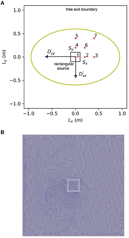
Figure 1. Illustration of simulation domain for 2D anisotropic diffusion verification problem with a rectangular source at the center, red symbols identify observation points and the olive-colored ellipse is a schematic representation of the contaminant plume (A) and mesh (B).
The simulation domain has a length of 2.0 m in the x- and y-direction, respectively. A Delaunay triangular mesh is used, with 6,423 discretization points and 12,560 cells, respectively. Seven observation points are selected, with coordinates in meters (0.0, 0.0), (0.2, 0.2), (0.4, 0.4), (0.0, 0.2), (0.0, 0.4), (0.2, 0.2) and (0.4, 0.4), respectively. The time step ranges from 1.0 × 10⁻¹⁰ to 1.0 × 10⁻² years. The parameters of the 2-D anisotropic diffusion problem are summarized in Table 1. Three different scenarios with an anisotropy ratio of 1:1, 10:1 and 100:1 are considered to study the spatiotemporal change of solute concentrations.
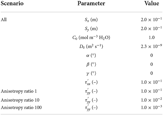
Table 1. Model parameters for 2-D anisotropic diffusion verification problem.
Without loss of generality, the normalized concentration (C/C0) is used throughout the analysis. The results obtained from the analytical and numerical solutions are shown in Figure 2. For both isotropic diffusion (anisotropy ratio = 1) and anisotropic diffusion (anisotropy ratio = 10 and 100), the numerical solution is in good agreement with the analytical solution.
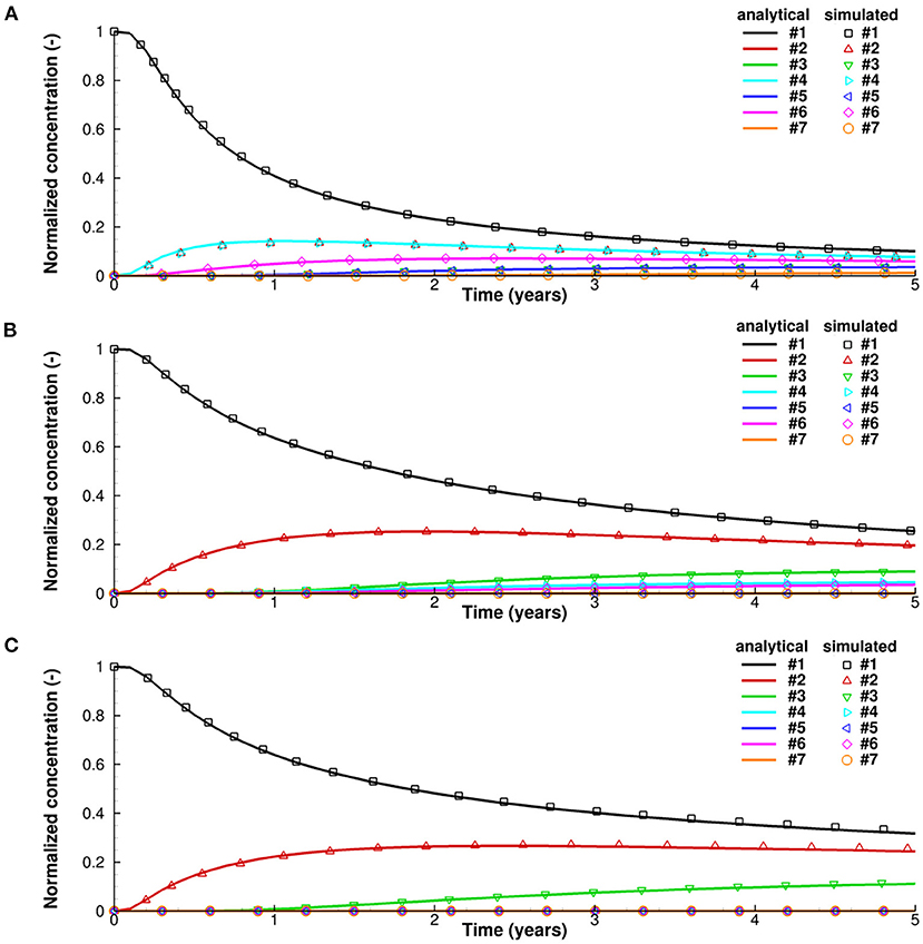
Figure 2. Normalized concentration change over time at specified observation points for 2D anisotropic diffusion verification problem, (A) with anisotropy ratio , (B) with anisotropy ratio , and (C) with anisotropy ratio .
Verification against 3-D analytical solution
Similar to the 2-D scenario, the analytical solution of 3-D anisotropic diffusion is obtained for a point source at the center (0, 0, 0) of a simulation domain with infinite extent in x-, y- and z-directions (Paladino et al., 2018):
where V0 (m3) is the volume of the instantaneous point source.
Due to the symmetry, only 1/8 of the 3-D spherical source is considered in the simulations, as shown in Figure 3. The volume of the source is therefore also scaled to 1/8 of the full domain source volume. The radius of the sphere is large enough to mimic an infinite boundary and concentrations at the boundary remain very low and do not affect concentrations at the observation points. A Delaunay tetrahedral mesh is used, with 9,672 discretization points and 45,002 cells, respectively. The simulation domain has a length of 100 m in x-, y- and z-directions. Mesh resolution ranges from 0.01 m at the center, where the source is located, to 10 m at the outer boundaries. Three different scenarios with anisotropy ratios of 5:1:1, 5:2:1, 10:5:1 are considered. Five observation points are selected, with coordinates in meters (0.126, 0.165, 0.491), (0.515, 0.218, 0.448), (0.15, 0.0, 0.0), (0.0, 0.15, 0.0) and (0.0, 0.0, 0.15), respectively. The time step ranges from 1.0 × 10⁻¹⁵ to 1.0 × 10² days. The parameters for the 3-D anisotropic diffusion verification problem are shown in Table 2.
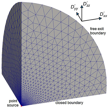
Figure 3. Illustration of simulation domain for 3-D anisotropic diffusion verification problem with tetrahedral mesh.
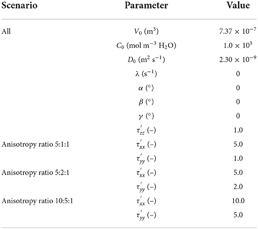
Table 2. Model parameters for 3-D anisotropic diffusion verification problem.
The results obtained from the analytical and numerical solutions are shown in Figure 4. For all anisotropy ratios the numerical solution provides a good match with the analytical solution. There are some discrepancies between the simulated results and analytical solution in the early stages when the concentration at the specified observation points begins to increase. This is mainly caused by numerical inaccuracies when quantifying the diffusive fluxes, which are more significant in a general mesh than a K-orthogonal mesh. Numerical inaccuracies in a tetrahedral mesh in 3-D space are larger than for a triangular mesh in 2-D space. However, these errors only occur at early time and do not affect the evolution of diffusion profiles in the long term. A sensitivity analysis with respect to mesh resolution has shown that these errors can be reduced by using a refined mesh with higher resolution. Detailed information on the effect of mesh resolution on the magnitude of error can be found in the Supplementary materials (Sections 5, 6). The numerical solution can therefore be considered sufficiently accurate.
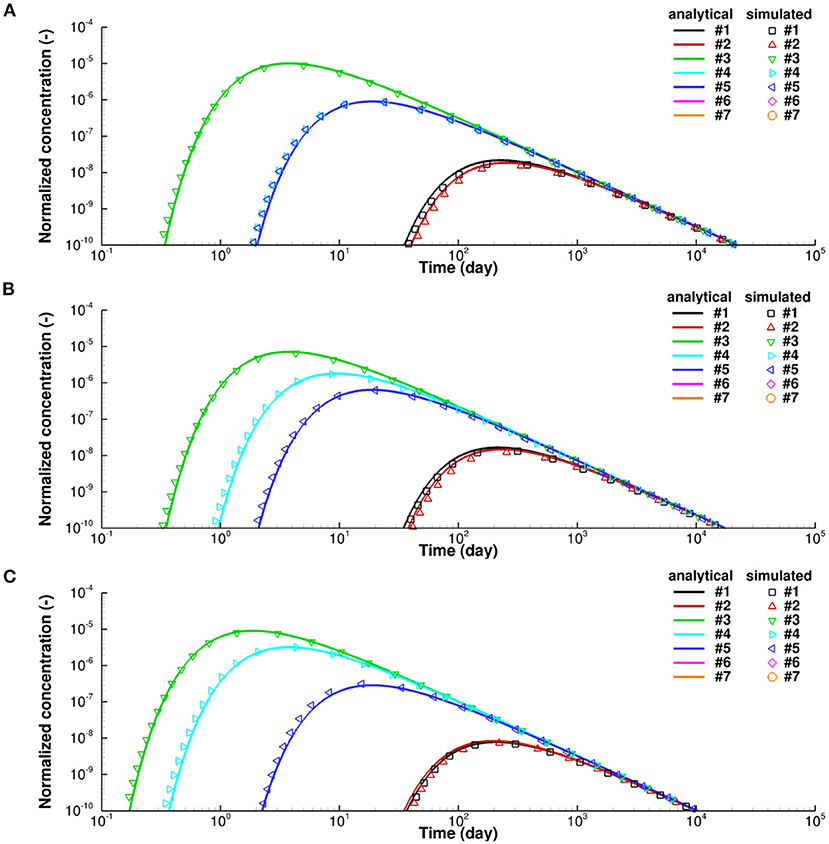
Figure 4. Normalized concentration changes over time at specified observation points for 3D anisotropic diffusion verification problem, (A) with anisotropy ratio , (B) with anisotropy ratio , and (C) with anisotropy ratio .
Modeling of local-scale diffusive solute transport – Mont Terri CI-D in-situ diffusion experiment
Overview of the Mont Terri CI-D in-situ diffusion experiment
The CI-D (diffusion across concrete/claystone interface) experiment conducted in the Mont Terri underground laboratory focuses on the characterization of diffusion-dominated solute transport from a constructed reservoir, through cementitious material, into the surrounding host rock, composed of anisotropic Opalinus Clay (OPA) (Jenni et al., 2014; Mäder et al., 2017; Bernard et al., 2020). An illustration of the experimental setup is shown in Figure 5. Two types of cementitious materials are contained in the simulation domain, including ordinary Portland cement (OPC) hosting the borehole and a low-pH concrete containing silica fume (ESDRED) (Bernard et al., 2020). Between the host rock and borehole is the excavation damage zone (EDZ), including 0.05 m inner part (iEDZ) and 0.1 m outer part (oEDZ). The spatial extent of the different materials ranges from 0.01 m to several meters.
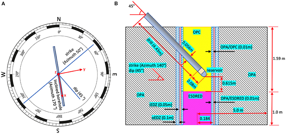
Figure 5. Illustration of in-situ experiment, (A) plan view and (B) section view.
The simulation domain contains several intersecting structures requiring the code to be able to deal with these complex conditions. The host rock (OPA) has a strike of azimuth of 50° and dip angle of 45°. The borehole has an orientation of azimuth of 170° and an inclination angle of 45° to the surface. The solute reservoir was placed at the end of the borehole, in which an artificial pore water (APW) system was installed. Solutes were circulated through the APW and diffused across the boundary of the reservoir into and through OPC. In this experiment, the injected tracer will migrate by isotropic diffusion through OPC, across the OPC/OPA interface and then continue by anisotropic diffusion through OPA, with faster transport parallel to the bedding than perpendicular to the bedding (Van Loon et al., 2004; Gimmi et al., 2014).
Model setup and parameters
The implementation of anisotropic diffusion is challenging for this problem, due to the complex 3-D geometry involved in the experimental setup. The simulation domain consists of 410,443 points and 2,411,550 tetrahedral cells, with resolution ranging from 0.01 to 0.5 m, as shown in Figure 6. In this research, HTO was used as a tracer to study the effect of anisotropy on diffusion. Based on measured effective diffusion coefficients of HTO which range from 1.80 × 10⁻¹³ m2 s−1 in concrete, to 3.20 × 10⁻¹¹ m2 s−1 along the bedding and 5.44 × 10⁻¹² m2 s−1 perpendicular to the bedding in OPA (Van Loon et al., 2004; Marty et al., 2015), we derived tortuosity correction factors for the different materials. HTO has a half-life of 12.3 years, corresponding to a first order decay rate of 2.6 × 10⁻⁹ s−1, which was also considered in the simulations. For the comparative scenario with isotropic diffusion, an effective average diffusion coefficient was calculated as the arithmetic mean of the anisotropic diffusion coefficients in the three directions and a constant tortuosity correction factor was used for diffusion in all directions. Model parameters for the simulation of the in-situ experiment are shown in Table 3.
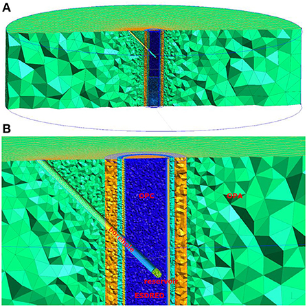
Figure 6. Illustration of simulation domain for in-situ experiment using tetrahedral cells, (A) the entire simulation domain, and (B) borehole region.
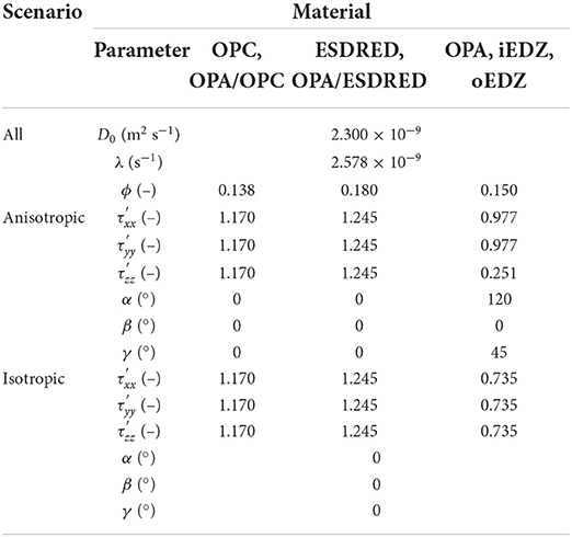
Table 3. Model parameters for simulation of Mont Terri CI-D in-situ diffusion experiment.
Results and discussion
The spatial distribution of solute concentrations for cases with and without consideration of dipping anisotropy are shown in Figure 7. At early time, the concentrations of HTO close to the source reservoir are similar for both cases, since the reservoir is surrounded by isotropic concrete, as shown by the 1.0 × 10⁻² contour for normalized concentrations in Figures 7A,C. However, after HTO enters the anisotropic material, concentration distributions for the case considering the effect of anisotropy reveal the directional effect associated with enhanced diffusion parallel to bedding and shorter migration distances in the direction perpendicular to the bedding, as can be seen in the 1.0 × 10⁻³ and 1.0 × 10⁻⁴ contours of normalized concentrations, for short-term and longer-term simulations, respectively. These results are consistent with previous findings (Van Loon et al., 2004; Gimmi et al., 2014).
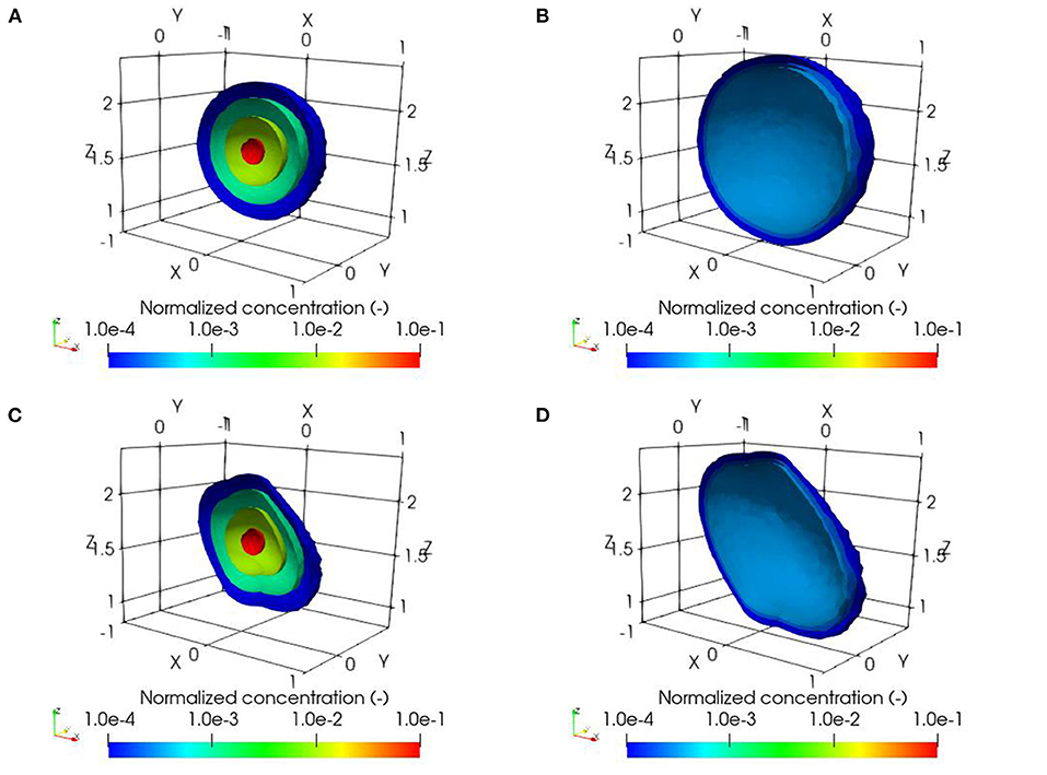
Figure 7. Simulated normalized concentration distributions of HTO for the in-situ diffusion experiment, (A) isotropic diffusion after 837 days, (B) isotropic diffusion after 1825 days, (C) anisotropic diffusion after 837 days, and (D) anisotropic diffusion after 1825 days.
To further analyze differences between the results with and without dipping anisotropy, we estimate the change of plume volume over time based on the dilution index (Kitanidis, 1994). In addition, we determine the transport distance of solute away from the source, which is taken as the maximum distance from the center of the reservoir to surrounding cells with normalized concentrations reaching 1.0 × 10⁻⁴. As shown in Table 4, the plume volumes considering dipping anisotropy are 2.1 and 5.1% smaller than for the isotropic case, after 837 days and 1825 days, respectively. On the other hand, the maximum transport distance away from the source is larger for the case with dipping anisotropy, compared to the isotropic case. The differences are 14.4 and 15.4% after 837 days and 1,825 days, respectively. Differences for the plume volumes become slightly more significant over time, as shown in Figure S.9 in the Supplementary materials, as the plume permeates deeper into the anisotropic material. However, the results indicate that dipping anisotropy only has a modest impact on long-term solute migration for the conditions considered.
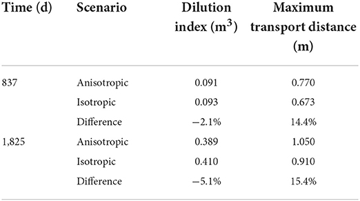
Table 4. Dilution index, representing simulated plume volume, and maximum transport distance for the Mont Terri CI-D in-situ diffusion experiment for anisotropic and equivalent isotropic scenarios.
The simulated concentrations of HTO in the reservoir are almost identical between the anisotropic diffusion scenario and the equivalent isotropic diffusion scenario over the 2,000 day simulation period, as shown in Figure 8A. The simulated results from both anisotropic and isotropic scenarios provide good agreement with the experimental observations, indicating that the total amount of solute migrating from the solute reservoir into the host rock is similar for both anisotropic diffusion and equivalent isotropic diffusion. Over the 2,000 day simulation period, the difference of HTO concentration in the reservoir between the anisotropic and isotropic scenarios increases, but not significantly, as shown in Figure 8B. As more solute passes through the isotropic cementitious material and enters the anisotropic rock matrix, the difference increases, but no more than 0.5% after 2,000 days.
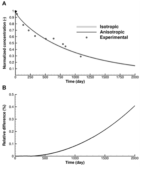
Figure 8. (A) Comparison of normalized concentrations of HTO in the source reservoir for the anisotropic diffusion scenario, equivalent isotropic diffusion scenario and experimental observations, (B) relative difference of simulated reservoir concentrations between anisotropic and equivalent isotropic diffusion scenarios.
Considering the relatively small differences between the results suggests that, in this situation, it can be sufficient to use the equivalent isotropic approximation, if the focus is on estimating mass loss from the reservoir. However, if the detailed tracer distribution within the rock matrix is of interest, anisotropy should be considered.
Modeling of far-field diffusive solute transport from a hypothetical deep geological repository (DGR)
Overview of the hypothetical DGR site
To study the effect of dipping anisotropy on long-term, far-field solute transport, a hypothetical deep geologic repository (DGR) in low permeability sedimentary rock is considered. The rock formations consist of sandstone, limestone, dolomite and shale, as shown in Figure 9A. All sedimentary rock layers have a strike of azimuth of 45° and a dip angle of 30°. The simulation domain has a horizontal length and width of 5 km and a vertical extent of 1 km. Within the simulation domain there are four sandstone layers, three dolomite layers, two shale layers and one limestone layer. Thicknesses of these layers, from earlier to later deposits, are 401, 540, 480, 540, 480, 360, 420, 480, 420, and 281 m, respectively. The dimensions of the DGR are assumed to be 400 × 400 × 20 m, located 500 m below the surface at the center of the 480 m thick shale layer. To investigate solute migration we assume part of the base of the DGR is damaged and solute is released from a 20 × 20 × 5 m region, as shown in Figures 9B,C.
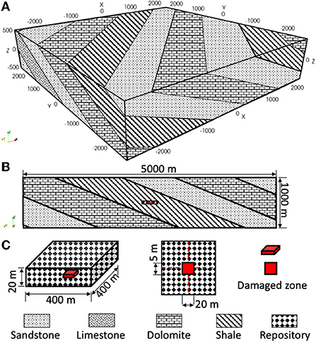
Figure 9. Illustration of sedimentary rock formations and repository location for a hypothetical DGR site, (A) rock formations in 3-D view, and (B) rock formations in cross-sectional view with DGR hosted in shale layer, and (C) dimensions of DGR and damaged region.
Model setup and parameters
The simulation domain consists of 1,257,523 discretization points and 1,220,736 hexahedral cells, with horizontal resolution ranging from 10 to 50 m and vertical resolution ranging from 5 to 25 m. The mesh surrounding the DGR site is refined with higher resolution of 10 m in the horizontal direction and 5 m vertically. The DGR site is assumed to be located in very low permeability material with a tortuosity factor set to 1.0 × 10⁻⁶. For these illustrative simulations, a conservative solute is released from the damaged zone, with an initial concentration of 1.0 mol m−3. The boundaries of the simulation domain are set to free exit boundary conditions which allows solute to exit once it reaches the boundary.
Dipping anisotropy is considered in the shale formation only. The other formations and the DGR are considered as isotropic. For the anisotropic simulation scenario, the tortuosity factor in the direction perpendicular to the bedding is 10 times smaller than in the direction parallel to the bedding. For the equivalent isotropic simulation scenario, the tortuosity factor is averaged arithmetically in the three directions. Detailed parameters for this illustrative test case are shown in Table 5.
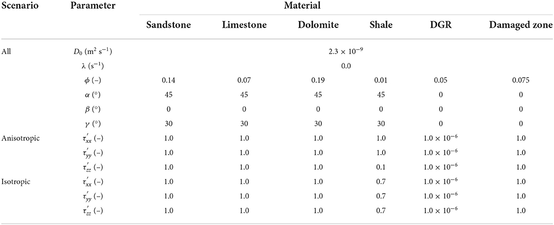
Table 5. Model parameters for solute diffusion from a hypothetical DGR site.
Results and discussion
The spatial distribution of solute concentrations shows significant differences between the anisotropic and equivalent isotropic simulation scenarios, as shown in Figure 10. The simulations indicate that solute migrates much farther along the bedding direction when dipping anisotropy is considered, compared to the equivalent isotropic simulation scenario where dipping anisotropy is ignored. More importantly, solute remains inside the shale layer when dipping anisotropy is considered, compared to the equivalent isotropic scenario where solute migrates into neighboring formations. The spatial distribution of solute concentrations demonstrates that it can be important to consider dipping anisotropy for long-term simulations.
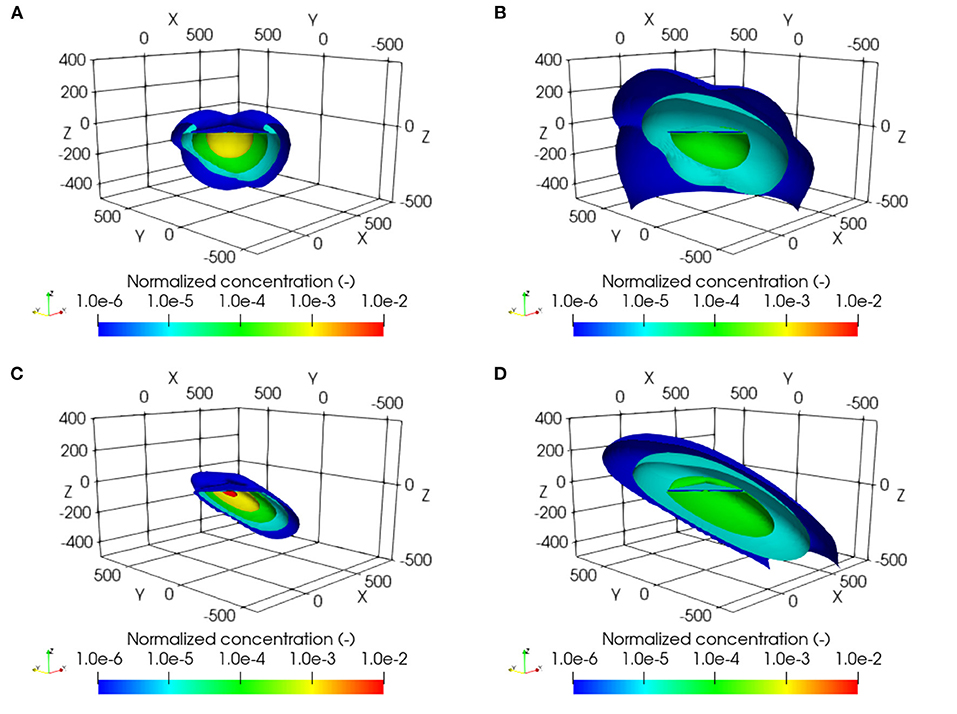
Figure 10. Simulated normalized concentration distributions of HTO for a hypothetical DGR site, (A) isotropic diffusion after 0.1 million years, (B) isotropic diffusion after 0.5 million years, (C) anisotropic diffusion after 0.1 million years, and (D) anisotropic diffusion after 0.5 million years.
The dilution index, representing the plume volume, and transport distances in x-, y-, and z-directions after 100,000 years and 500,000 years are shown in Table 6. We can see that after 100,000 years the plume volume is substantially smaller for the anisotropic case (by 19.0%). Differences of plume volumes between isotropic and anisotropic cases continue to increase over time and reach 39.4% after 500,000 years. Similar to the Mt Terri CI-D simulation, transport distances are determined based on the maximum distance from the center of the defect to surrounding cells with normalized concentrations reaching 1.0 × 10⁻⁴. Relative differences of transport distances in x-direction and y-direction show a larger plume extent for the case with dipping anisotropy, while the extent of the plume in z-direction is much smaller than for the isotropic case (Table 6). These results indicate that dipping anisotropy causes substantial differences on solute migration in both short-term and longer-term simulations. The temporal evolution of the dilution index can be found in Figure S.10 in the Supplementary Section 8.
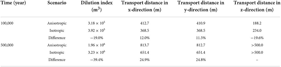
Table 6. Dilution index, representing simulated plume volume, and solute transport distances in x-, y- and z-directions for a hypothetical DGR site for anisotropic and equivalent isotropic scenarios.
Notably, differences between the anisotropic approach and the equivalent isotropic approach for the hypothetical DGR site simulation are significantly more pronounced than for the Mont Terri CI-D simulation. These discrepancies can be attributed to several circumstances. Firstly, in the case of the DGR simulation, the solute enters anisotropic material immediately after release from the source, while in the Mont Terri CI-D simulation, the source is hosted in isotropic material. In addition, the anisotropy ratio is much larger for the DGR site simulation, resulting in a stronger effect on transport directions. Furthermore, the fact that solute can enter neighboring layers with higher diffusivity in the isotropic DGR scenario, while this does not occur for the anisotropic scenario, has a substantial effect on plume volumes and transport distances.
Conclusions
In this research a fully 3-D unstructured grid code was developed for simulating diffusive solute transport in systems with complex geometry and dipping anisotropy. The code has been verified against analytical solutions for both 2-D and 3-D diffusion problems and the results have shown good agreement with the analytical solutions.
The code was then applied to simulate anisotropic diffusion for an in-situ diffusion experiment performed at the Mont Terri underground laboratory. In the long term, the spatial distribution of HTO concentrations show small differences between the anisotropic diffusion scenario and the equivalent isotropic diffusion scenario. The total plume volume based on the dilution index and transport distance away from the source are quite similar for the anisotropic and equivalent isotropic approaches, indicating that using the equivalent isotropic approach may provide an adequate approximation, especially if the focus is on estimating mass loss from the solute reservoir.
The code has also been applied to a hypothetical DGR scenario to illustrate long-term, far-field solute diffusion from a damaged zone. The simulations show that solute remains inside the low permeability shale layer within 500,000 years, when dipping anisotropy is considered, while under an equivalent isotropic condition, solute reaches a neighboring formation at much earlier time. The vertical transport distance and volume of the plume obtained with the anisotropic approach are much less than those obtained for an equivalent isotropic simulation. This significant difference indicates the importance of considering dipping anisotropy, especially in the long-term, particularly in layered systems.
The code developed provides a versatile tool to simulate anisotropic diffusion in layered systems containing complex subsurface structures. As implemented, future simulations can be expanded to include heterogeneity and biogeochemical reactions.
Data availability statement
The original contributions presented in the study are included in the article/Supplementary material, further inquiries can be directed to the corresponding author.
Author contributions
DS: conceptualization, methodology, code development, data analysis, and writing and editing. MX: methodology, data analysis, and writing—review and editing. KUM: supervision and writing—review and editing. KTBM: co-supervision and writing—review and editing. All authors contributed to the article and approved the submitted version.
Funding
This research was supported by the Nuclear Waste Management Organization (NWMO), Canada.
Acknowledgments
The authors would like to acknowledge Mt Terri experiment team for providing data and support. The authors would also like to acknowledge the UBC EOAS department, WestGrid and Compute Canada for providing computing hardware, software, and technical support.
Conflict of interest
The authors declare that the research was conducted in the absence of any commercial or financial relationships that could be construed as a potential conflict of interest.
Publisher's note
All claims expressed in this article are solely those of the authors and do not necessarily represent those of their affiliated organizations, or those of the publisher, the editors and the reviewers. Any product that may be evaluated in this article, or claim that may be made by its manufacturer, is not guaranteed or endorsed by the publisher.
Supplementary material
The Supplementary Material for this article can be found online at: https://www.frontiersin.org/articles/10.3389/frwa.2022.974145/full#supplementary-material
References
Bennett, J. P., Haslauer, C. P., and Cirpka, O. A. (2017). The impact of sedimentary anisotropy on solute mixing instacked scour-pool structures. Water Resour. Res. 2016, WR019665. doi: 10.1002/2016WR019665
Bernard, E., Jenni, A., Fisch, M., Grolimund, D., and Mäder, U. (2020). Micro-X-ray diffraction and chemical mapping of aged interfaces between cement pastes and Opalinus Clay. Appl. Geochemistr. 115, 104538. doi: 10.1016/j.apgeochem.2020.104538
Charbeneau, R. J. (2006). Groundwater Hydraulics And Pollutant Transport. New York, NY: Waveland Pr Inc.
Craig, J. R. (2008). Analytical solutions for 2D topography-driven flow in stratified and syncline aquifers. Adv. Water Resour. 31, 1066–1073. doi: 10.1016/j.advwatres.2008.04.011
Fan, Y., Toran, L., and Schlische, R. W. (2007). Groundwater flow and groundwater-stream interaction in fractured and dipping sedimentary rocks: insights from numerical models. Water Resour. Res. 43, 4864. doi: 10.1029/2006WR004864
Gimmi, T., Leupin, O. X., Eikenberg, J., Glaus, M. A., Loon, L. R. V., Waber, H. N., et al. (2014). Anisotropic diffusion at the field scale in a 4-year multi-tracer diffusion and retention experiment—I: insights from the experimental data. Geochimica et Cosmochimica Acta 125, 373–393. doi: 10.1016/j.gca.2013.10.014
Henderson, D. M. (1977). Euler Angles, Quaternions, and Transformation Matrices for Space Shuttle Analysis, Contractor Report (CR). Available online at: https://ntrs.nasa.gov/citations/19770019231
Hoaglund, J. R., and PoIllard, D. (2003). Dip and anisotropy effects on flow using a vertically skewed model grid. Groundwater 41, 841–846. doi: 10.1111/j.1745-6584.2003.tb02425.x
Holleman, R., Fringer, O., and Stacey, M. (2013). Numerical diffusion for flow-aligned unstructured grids with application to estuarine modeling. Int. J. Numeric. Methods Fluids 72, 1117–1145. doi: 10.1002/fld.3774
Jenni, A., Mäder, U., Lerouge, C., Gaboreau, S., and Schwyn, B. (2014). In situ interaction between different concretes and opalinus clay. Physics Chemistr. Earth, Parts A/B/C 70–71, 71–83. doi: 10.1016/j.pce.2013.11.004
Kerner, C. (1992). Anisotropy in sedimentary rocks modeled as random media. Geophysics 57, 564–576. doi: 10.1190/1.1443270
Kitanidis, P. K. (1994). The concept of the dilution index. Water Resour. Res. 30, 2011–2026. doi: 10.1029/94WR00762
Lichtner, P. C., Kelkar, S., and Robinson, B. (2002). New form of dispersion tensor for axisymmetric porous media with implementation in particle tracking. Water Resour. Res. 38, 100. doi: 10.1029/2000WR000100
Lippmann-Pipke, J., Gerasch, R., Schikora, J., and Kulenkampff, J. (2017). Benchmarking PET for geoscientific applications: 3D quantitative diffusioncoefficient determination in clay rock. Comput. Geosci. 1, 2. doi: 10.1016/j.cageo.2017.01.002
Mäder, U., Jenni, A., Lerouge, C., Gaboreau, S., Miyoshi, S., Kimura, Y., et al. (2017). 5-year chemico-physical evolution of concrete–claystone interfaces, Mont Terri rock laboratory (Switzerland). Swiss J. Geosci. 110, 307–327. doi: 10.1007/s00015-016-0240-5
Marty, N. C. M., Bildstein, O., Blanc, P., Claret, F., Cochepin, B., Gaucher, E. C., et al. (2015). Benchmarks for multicomponent reactive transport across a cement/clay interface. Computat. Geosci. 19, 635–653. doi: 10.1007/s10596-014-9463-6
Mayer, K. U., Frind, E. O., and Blowes, D. W. (2002). Multicomponent reactive transport modeling in variably saturated porous media using a generalized formulation for kinetically controlled reactions. Water Resour. Res. 38, 1174. doi: 10.1029/2001WR000862
Paladino, O., Moranda, A., Massabò, M., and Robbins, G. A. (2018). Analytical solutions of three-dimensional contaminant transport models with exponential source decay. Groundwater 56, 96–108. doi: 10.1111/gwat.12564
Qin, R., Wu, Y., Xu, Z., Xie, D., and Zhang, C. (2013). Numerical modeling of contaminant transport in a stratified heterogeneous aquifer with dipping anisotropy. Hydrogeol. J. 21, 1235–1246. doi: 10.1007/s10040-013-0999-7
Rousseau, M., and Pabst, T. (2021). Analytical solution and numerical simulation of steady flow around a circular heterogeneity with anisotropic and concentrically varying permeability. Water Resour. Res. 57, e2021WR029978. doi: 10.1029/2021WR029978
Samper, J., Yang, C., Naves, A., Yllera, A., Hernández, A., Molinero, J., et al. (2006). A fully 3-D anisotropic numerical model of the DI-B in situ diffusion experiment in the Opalinus clay formation. Physic. Chemistr. Earth Parts A/B/C 31, 531–540. doi: 10.1016/j.pce.2006.04.017
Su, D., Mayer, K. U., and MacQuarrie, K. T. B. (2017). Parallelization of MIN3P-THCm: A high performance computational framework for subsurface flow and reactive transport simulation. Environ. Modell. Softw. 95, 271–289. doi: 10.1016/j.envsoft.2017.06.008
Su, D., Mayer, K. U., and MacQuarrie, K. T. B. (2020). Numerical investigation of flow instabilities using fully unstructured discretization for variably saturated flow problems. Adv. Water Resour. 143, 103673. doi: 10.1016/j.advwatres.2020.103673
Su, D., Mayer, K. U., and MacQuarrie, K. T. B. (2021). MIN3P-HPC: a high performance unstructured grid code for subsurface flow and reactive transport simulation. Mathematic. Geosci. 53, 517–550. doi: 10.1007/s11004-020-09898-7
Tournassat, C., and Steefel, C. I. (2021). Modeling diffusion processes in the presence of a diffuse layer at charged mineral surfaces: a benchmark exercise. Computat. Geosci. 25, 1319–1336. doi: 10.1007/s10596-019-09845-4
Van Loon, L. R., Soler, J. M., Müller, W., and Bradbury, M. H. (2004). Anisotropic diffusion in layered argillaceous rocks: a case study with opalinus clay. Environ. Sci. Technol. 38, 5721–5728. doi: 10.1021/es049937g
Yager, R. M., Voss, C. I., and Southworth, S. (2009). Comparison of alternative representations of hydraulic-conductivity anisotropy in folded fractured-sedimentary rock: modeling groundwater flow in the Shenandoah Valley (USA). Hydrogeol. J. 17, 1111–1131. doi: 10.1007/s10040-008-0431-x
Yan, S. (2019). Non-negative numerical solutions of the two-dimensional full-tensor diffusion/dispersion problems using flux-corrected transport, and implementation for the groundwater transport simulator MT3DMS (M.S. Thesis). University of Illinois at Urbana-Champaign, Urbana-Champaign, IL, United States. Available online at: https://www.ideals.illinois.edu/items/112029
Keywords: dipping anisotropy, solute transport, heterogeneous, porous media, sedimentary rock
Citation: Su D, Xie M, Mayer KU and MacQuarrie KTB (2022) Simulation of diffusive solute transport in heterogeneous porous media with dipping anisotropy. Front. Water 4:974145. doi: 10.3389/frwa.2022.974145
Received: 20 June 2022; Accepted: 13 September 2022;
Published: 25 October 2022.
Edited by:
Marwan Fahs, National School for Water and Environmental Engineering, FranceReviewed by:
Giovanni Michele Porta, Politecnico di Milano, ItalyBehshad Koohbor, Université de Montpellier, France
Copyright © 2022 Su, Xie, Mayer and MacQuarrie. This is an open-access article distributed under the terms of the Creative Commons Attribution License (CC BY). The use, distribution or reproduction in other forums is permitted, provided the original author(s) and the copyright owner(s) are credited and that the original publication in this journal is cited, in accordance with accepted academic practice. No use, distribution or reproduction is permitted which does not comply with these terms.
*Correspondence: Danyang Su, dsu@eoas.ubc.ca