Laser-induced breakdown spectroscopy as an analytical tool for total carbon quantification in tropical and subtropical soils: evaluation of calibration algorithms

GRAPHICAL ABSTRACT

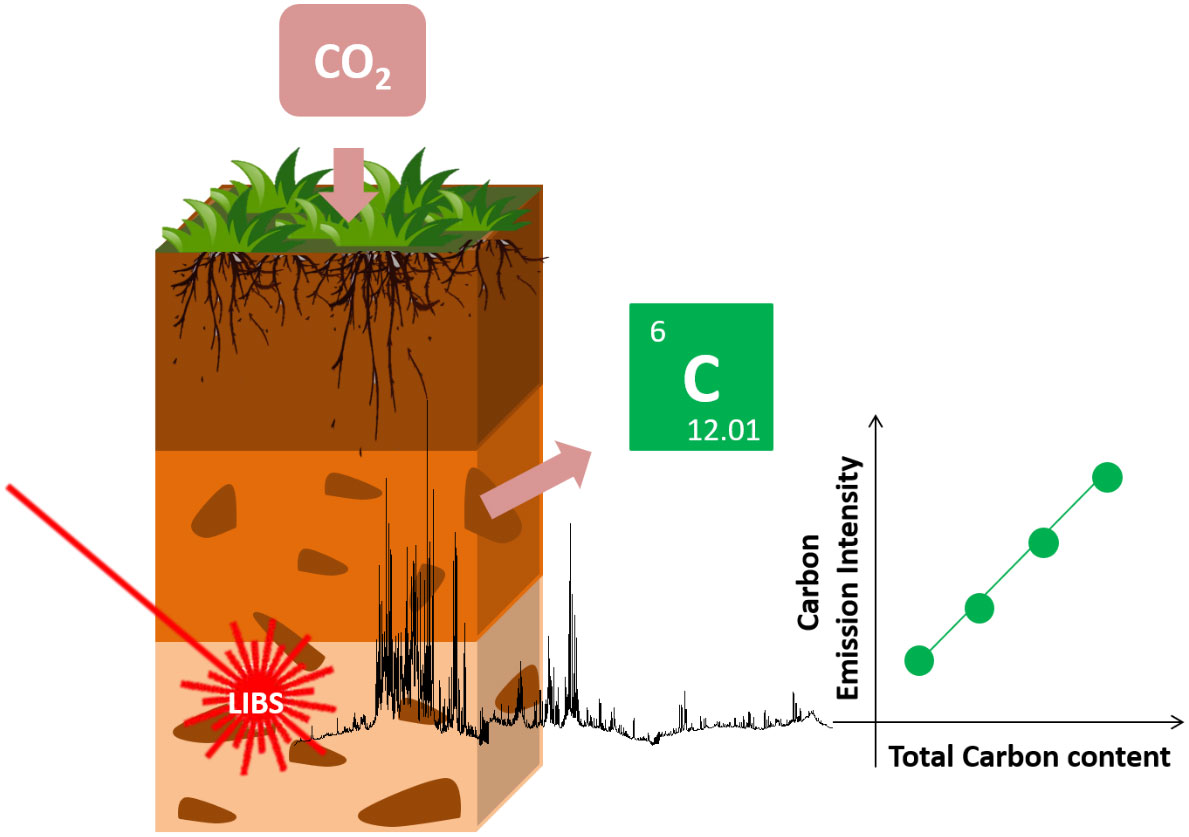
Graphical Abstract

1 Introduction

Soil is essential in the biogeochemical cycle of carbon, highlighting its role in the stabilization stage of carbon (C) as organic matter. In recent years in tropical and subtropical Brazilian regions, it has been possible to demonstrate that conservative tillage practices, such as no-tillage with grain production, well-managed pastureland, and integrated crop-livestock-forest systems, can promote excellent results in C mitigation from greenhouse gas emissions (GGE) by soil C sequestration (1–5). Most of the results available on soil C sequestration in Brazil were obtained in long-term field experiments conducted by research institutions. One of the few results with data from private farms was obtained by Ferreira et al. (2021) (6) from the southern region of Brazil, which has a subtropical climate, demonstrating that similar results can be generated in real farm conditions. Therefore, worldwide on-farm research must be stimulated considering the growing interest in the soil C credit market (7).

Specifically in tropical regions, Brazil leads in recent and competitive agriculture by incorporating agricultural land mainly in the savannah biome (called Cerrado), with 200 million hectares. A combination of conservative tillage practices, including no-tillage, lime, and fertilizer use, was used to correct acidity and simultaneously reduce the negative impact for plants in soils with high soil aluminum content, as well as to improve soil fertility and reduce the erosion process. These methods have also demonstrated good conditions to identify soil carbon sequestration situations, mitigating GGE (2), aligned with the “4 per 1000” global initiative (8).

Additionally, C stabilization as soil organic matter (SOM), preferably with a high degree of humification, contributes to C storage in soils and can provide excellent benefits in food production, improving the physicochemical properties of the soil. This is beneficial as soil fertility, due to an increase in cation exchange capacity (CEC), is also very much needed in tropical soils due to dominant kaolinite clay, with a 1:1 type, with low CEC (1). All these conditions, including the increase in the soil C content and the SOM stabilization, are relevant to consolidating the soil carbon credit market that can provide additional remuneration for farmers, stimulating the adoption of conservative tillage practices (9, 10).

The monitoring of total C in the soil can be done using analytical techniques that allow ex situ methods (wet combustion, for example), in situ methods (inelastic neutral scattering -INS, for example), and methods that would allow it to be developed in both places (for example, using near-infrared spectroscopy–NIRS) (10, 11). Among these methods, the dry combustion automated elemental analyzer is probably the most used analytical technique for C determination in soils due to its high precision. However, this technique has a high analytical cost due to its consumable materials, which can increase the analysis cost and limit its use in continuously monitoring large amounts of soil samples (10).

Thus, low-cost analytical techniques and high analytical frequency, which provide satisfactory accuracy and precision, must still be evaluated and implemented for C determination in samples of different types of soils. In this context, laser-induced breakdown spectroscopy (LIBS) presents many prerequisites that can contribute to the speed of soil analysis to determine total C (12–14). With these values obtained, LIBS can be used to assess the soil C stock that farmers can later trade as carbon credits, for example. LIBS is a photonic technique that uses a pulsed laser [usually solid-state ns or fs lasers (e.g., Nd : YAG lasers)] to analyze soil samples. The focused laser pulse ablates micrograms of the sample and enables the formation of a plasma, whose temperature is approximately 10,000 K at the time of collection of the analytical signal. Thermal energy promotes electronic transitions (excitation) of atoms, ions, and molecular constituents of the sample and is present in the formed plasma. It is possible to obtain a LIBS emission spectrum when returning to the fundamental state (13, 15). These species emit characteristic radiations of each species present (as a fingerprint), which are collected by an optical fiber and sent to the spectrometer and detector. Considering the stoichiometric ablation, the local thermodynamic equilibrium, and the optically thin emission, it is possible to correlate the area or intensity of the emission lines (wavelength) with the concentration of elements present in the soil sample (13–15).

Recently, Verra, a world reference certifier in the carbon market for creating voluntary carbon standards (VCS), approved the LIBS technique for soil C measurement, along with other emerging proximal sensing technologies (NIRS, mid-infrared spectroscopy - MIR, visible-NIRS and INS), which have shown to hold promise for streamlining soil organic C measurement. This technique guarantees the origin of verifiable carbon credit units with a high-quality standard in the voluntary market through a global registry platform that takes care of credits (16).

The LIBS technique allows the direct analysis of soil samples, or with minimal sample preparation (such as preparation of soil pellets), fast spectrum acquisition (< 1 s), and ex situ analysis of the soil, in addition to C determination, which allows simultaneous multielemental determination (14, 17). This technique works without needing consumable materials (such as tin capsules, high-purity gas, or columns with appropriate resins used in the reference technique for C determination in soils, CHNS elemental analyzer) (10). It also involves minimal waste generation with relatively easy disposal (10), unlike colorimetric or volumetric methods, which use Cr₂O₇^2- and H₂SO₄ solutions to oxidize SOM. Furthermore, as demonstrated in the study by Knadel et al., 2017 (18), lower prediction errors for most properties (texture and soil organic carbon) were obtained using LIBS for Danish soils that are predominantly sandy and using the spiking method (19), rendering it an equally good or even a more accurate technique for soil properties’ determination than the well-established vis-NIRS method.

However, the physicochemical complexity of tropical soils is a challenge in LIBS analysis (and in other photonic techniques, such as NIRS, which employs the analyses of the solid samples) (20, 21) due to the heterogeneity of the matrix of soil samples (e.g., texture and type of soil), and the high content of aluminum and iron oxides and hydroxides that can contribute as spectral interference in the main carbon emission lines at 193.03 nm and 247.86 nm (17, 22). As the soil sample is analyzed entirely (analyte and matrix in the same ablated portion) by LIBS, the variability of the soil matrix can promote linearity deviations in calibration models used in the quantification of total C (13, 14, 22). In some cases, specific calibration models must be obtained for sets of soils depending on the texture of the analyzed samples, granulometry, or localized sets as proposed by Segnini et al. (2014) (23) using LIBS, and by Brunet et al. (2007) (20) using NIRS, respectively, making the method laborious.

Thus, it is essential to evaluate calibration strategies and the proposition of “universal calibration models” that allow for overcoming the matrix effects, considering the high variability of the matrix of different types of soils, textures, and granulometry, allowing the reliable determination of the C content in samples of soils. Several calibration strategies of the LIBS method are reported in the scientific literature for the determination of total C in soils, such as (i) internal standardization (23, 24), (ii) partial least squares regression (12, 25), and (iii) multiple linear regression (12). All calibration strategies have advantages and limitations in their use and should be chosen based on their intrinsic modeling characteristics, analytes, and sample complexity to obtain the lowest error of the prediction.

In this context, we evaluated the accuracy of four calibration strategies, namely matrix-matching calibration (MMC), MMC with inverse regression (IR), multiple linear regression (MLR), and artificial neural network (ANN), for the proposition of calibration models aiming for total C determination by LIBS. An extensive set of different Brazilian tropical and subtropical soil types (1,019 soil samples) was analyzed using LIBS so that the matrix heterogeneity of these soil samples could be representative in the calibration models. Additionally, a critical discussion was made between the advantages and limitations of LIBS compared to the CHNS elemental analyzer in soil C quantification. These results are part of a pioneering project in Brazil called PRO Carbon, with a large set of farms evaluated with the aim to stimulate and give scientific and technological support to low-carbon agriculture in grain production areas in a joint project conducted by the Brazilian Agricultural Research Corporation (Embrapa), a public research institution, and Bayer company (led by a Brazilian branch). Considering the importance of Brazil in the soil C credit market scenario, this study makes it possible to demonstrate at full scale the challenges and advantages of using this spectroscopic technique to measure total C in tropical and subtropical soils of private farms.

2 Materials and methods

2.1 Instrumentation

The LIBS measurements were performed using single-pulse LIBS at 1064 nm (Q-switched Ultra, Quantel), Supplementary Figure S1, in the laboratory. The 1064 nm ND : YAG laser pulse had a maximum energy of 75 mJ, a width of 6 ns, and a repetition rate of 20 Hz. A spectrometer (Ocean Optics) was used to detect and select wavelengths from 189 to 966 nm. The pulse energy was 75 mJ, the delay time between the pulse and acquisition was 1.5 μs, and the acquisition gate width was 1 ms. For each sample, 30 spectra were acquired from different regions of the pellet to minimize sample microheterogeneity and to obtain a representative analysis. This is an automated LIBS system, equipped with a carrousel with 30 sample holder places and the capacity to measure 100 samples per hour, developed in partnership between Embrapa Instrumentação and startup Agrorobótica, both located in São Carlos city, São Paulo state, Brazil.

The reference values of the total C content of soil samples were obtained from a Perkin-Elmer 2400 CHNS analyzer series II using a standard of acetanilide with content known as C. Soil samples were weighed directly in consumable tin capsules using an analytical balance for direct mass acquisition. The tin capsules were closed and inserted into the analyzer furnace.

2.2 Collection and preparation of soil samples

A total of 1,019 agricultural and native vegetation soil samples from three Brazilian biome areas, Cerrado (typical savannah native vegetation), Atlantic Forest, and Pampa, were collected from 11 different farms (Figure 1), with a soil carbon content ranging from 0.23 to 8.78 wt% C, as determined using the CHNS analyzer. In Supplementary Table S1 of the Supplementary Material, the information is shown regarding the location, biome, management system, number of samples, number of soil samples each farm used in the calibration and validation sets, and the maximum, minimum, and average values for the parameters clay content (%), soil density (g cm^-3), and total C (wt% C) of soil samples from each farm in the study. In each farm, soil samples from agricultural conservative tillage (no tillage) and native vegetation areas were collected to compose the sample bank. The agricultural areas for soil sampling were selected because they were close to native forest areas within the farm (to minimize the textural variability of sampling points between the two areas).

Figure 1

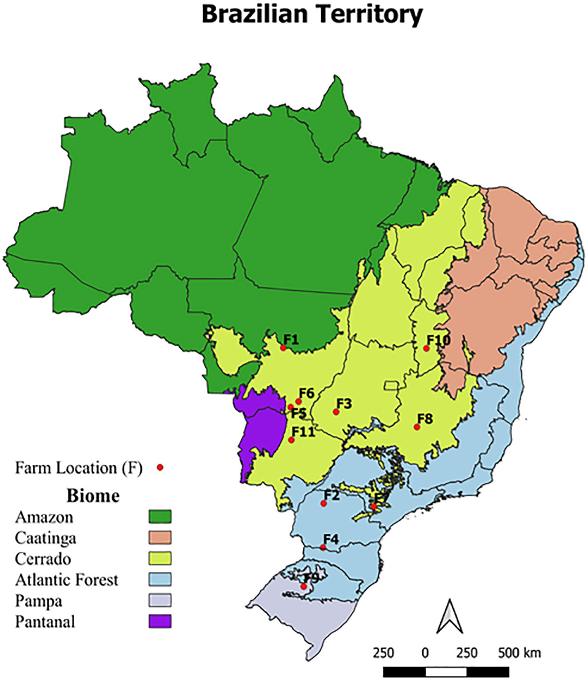
Figure 1 Geographic location of the 11 farms where 1,019 soil samples were collected for LIBS analysis.

One soil sample was collected per depth layer (approximately 500 cm³) at the following depths: 0–5, 5–10, 10–20, 20–30, 30–40, 40–60, 60–80, and 80–100 cm. In an agricultural area (under no-tillage) of approximately 35 hectares, and in the native forest area, eight and four trenches, respectively, were opened to collect soil in the different layers. All soil samples were collected before the establishment of a new crop, in the beginning of second half of 2020 (July/August). Currently in Brazil it is usual to have two crops’ cultivation sessions in one year, and the previous harvest session was concluded in June. The generally used combination is soybean (September-January) and corn (February-June). These samples were dried and homogenized (2 mm) for further analysis. The collection of samples in the soil profile is a strategy used to ensure the variability and representativeness of the matrix of soil samples because it is a significant analytical challenge for direct analysis and the development of a quantitative method of C by LIBS. The soil density was determined using volumetric cylinder methodology (26) (cylinders of 100 cm³, n = 2). Soil texture was determined, and soil samples were classified based on the United States of Agriculture (USDA) textural triangle (27).

Among the areas evaluated, there were none with poorly developed soil or an excessive or significant presence of rock fragments. A few rock fragments could be present in the samples and, in these cases, such fragments are excluded in the first stage of preparation, since they generally do not pass through the 2 mm mesh used in sieving and breaking up aggregates. For LIBS analysis, approximately 5.5 g of each sample (2 mm granulometry) was converted into soil pellets using a hydraulic press. The pellet is the pressed soil sample, as presented in Figure 2, in a specific aluminum metallic support, as the sample holder. Metallic supports were used to make pellets and to keep all samples cohesive. The soil samples were homogenized, and 10 mg of sample (n = 2) was encapsulated in tin capsules to determine total C by dry combustion (CHNS Perkin-Elmer analyzer).

Figure 2

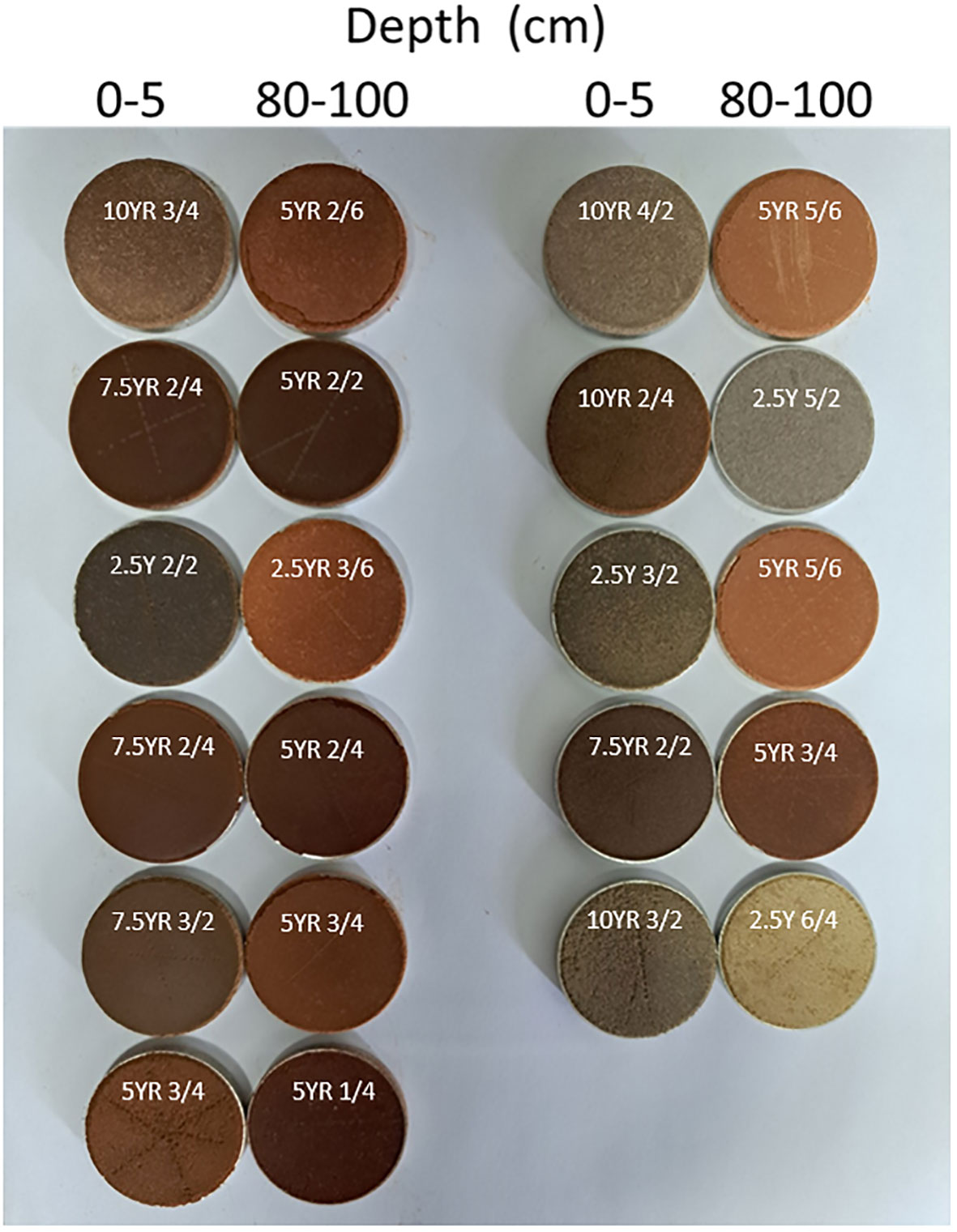
Figure 2 Digital image and classification by Munsell color system of some soil pellets that were analyzed by LIBS.

Some soil samples (at depths of 0–5 cm and 80–100 cm) from different systems (agricultural areas or native forests) of each of the 11 farms were randomly selected to demonstrate the different colors of the analyzed soils. Digital images were obtained using a smartphone camera and classification by Munsell color system, Figure 2.

2.3 Spectral pretreatment

The performance of the models is closely related to the spectral pretreatment used. Figure 3A shows a characteristic LIBS spectrum obtained from a soil sample. The models were built from the selection of 296 variables (wavelengths) referring to the intensities of the emission lines covering 192.04 to 194.97 nm (54 variables) for the C I 193.03 nm emission line, 197.60 to 199.95 nm (44 variables) for Al II 198.99 nm emission line, 277.45 to 286.68 nm (198 variables) for Mg II 279.55 nm, and Mg II 280.27 nm and Mg I 285.21 nm emission lines, respectively. The spectral pretreatments were performed using software developed in Python programming language. The baseline correction and, posteriorly, the Lorentzian fit (28) were initially made for all spectral ranges of the emission lines selected in the study. For the C I 193.03 line, it was necessary to perform spectral deconvolution due to Al II 193.58 nm line interference to minimize this spectral interference (22). The area of the emission lines of the monitored elements was calculated (C I 193.03 nm, Al II 198.99 nm, Mg II 279.55 nm, Mg II 280.27 nm, and Mg I 285.21 nm). For univariate calibration models, the average of the values obtained from the spectral pretreatments was used to minimize spectral fluctuations from the analysis of samples by LIBS and to improve the predictability of the models calculated.

Figure 3

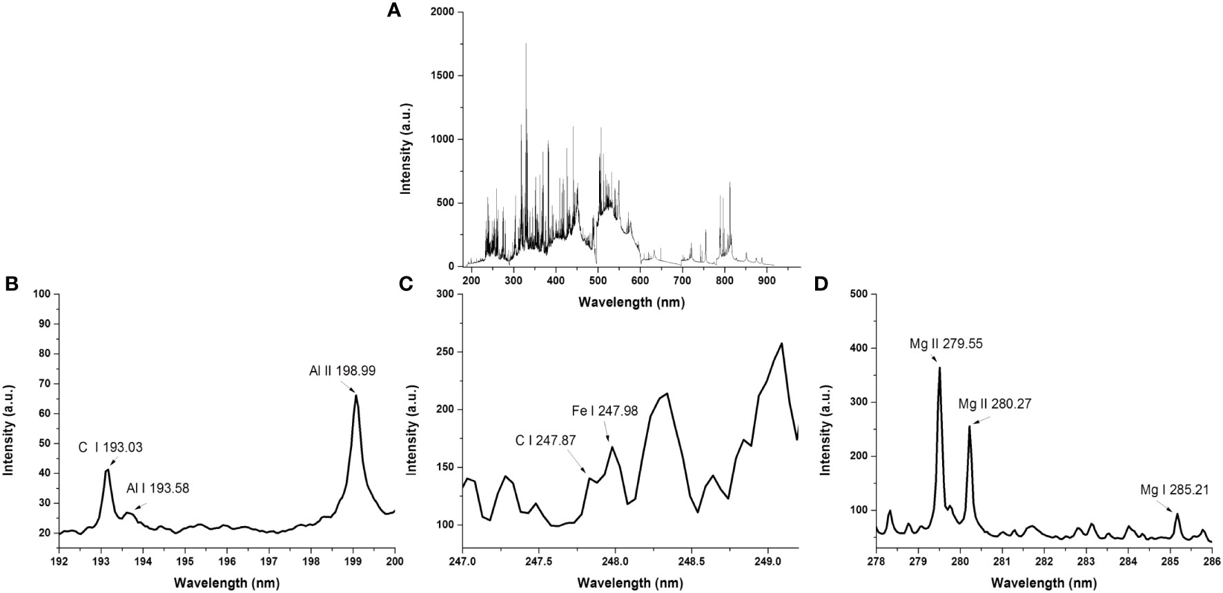
Figure 3 LIBS typical spectrum obtained from a soil sample (A), highlighting the spectral interferences in the emission lines of C I 193.03 nm (B), C I 247.87 nm (C), and the (D) profile of Mg lines used in the calculation of plasma temperature and self-absorption indices.

2.4 Calibration models

Four calibration models (two univariate and two multivariate models) were obtained to determine the total C in the soil. All models evaluated were built using 713 soil samples randomly chosen to compose a calibration set and 306 soil samples randomly chosen to compose an external validation set (to verify the predictive capacity of the models) [see boxplot and violin box of total C contents of the two sets, Supplementary Figures S1 and S3, summary statistics of total C contents at each sampling depth (0 to 100 cm)], in the Supplementary Material. The selection of soil samples used in the calibration set were chosen randomly, in order not to present trends that could reflect on the magnitude of errors and other figures of merit calculated. Furthermore, as the set is large and representative, it is possible to test the model (prediction set) with only a percentage of the samples, also randomly chosen. Soil samples collected from 0 to 100 cm depths with different textures were used in both sets.

In calibration using (I) MMC (29), a set of soil samples was used as solid calibration standards (713 soil samples), with known reference values for total C content. A calibration model using least squares regression was proposed to monitor the emission line C I 193.03 nm and perform spectral deconvolution. The dependent variable was the intensity of the C emission line obtained. As the independent variable, the reference values of the C content were previously determined [C emission signal = function (concentration)]. In (II) MMC–inverse regression (30), the least squares regression was obtained using the reference values of the C content as the dependent variable and the intensity of the C emission line obtained as the independent variable [concentration = function (C emission signal)].

In addition to the two univariate calibration models described, two multivariate models were evaluated. In (III) MLR, three independent variables were used: i) the analyte line intensity (C I 193.03 nm), ii) the self-absorption index, and iii) the plasma temperature index. The self-absorption and plasma temperature index are calculated using the ratio of the intensities of Mg emission lines [Figure 3D (self-absorption index: Intensity Mg II 279.55 / Intensity Mg II 280.27, and plasma temperature index: Intensity Mg II 280.27 / Intensity Mg I 285.21)] and were used for each analyzed soil sample (31). These indices were used to evaluate their contributions to minimizing matrix effects. As preprocessing, the discrete variables were autoscaled by standard deviation. The C content in the soils used as standards was the response (regression vector) of the model. The models were trained using routines in MATLAB software version 2017b (MathWorks, Natick, MA).

The (IV) ANN model was built using all 296 variables (wavelengths) mentioned above from intensities around the emission lines for C I 193.03 nm, Al II 198.99 nm, Mg II 279.55 nm, Mg II 280.27 nm, and Mg I 285.21 nm. The artificial neural network (ANN) used was a multilayer perceptron (MLP) with an architecture of 296 variables in the input layer, 50 neurons in the hidden layer, and one in the output layer related to the carbon content. The rectified linear unit (ReLU) activation function was used for all neurons. The MLP was trained using the backpropagation algorithm (32). The backpropagation parameters and the MLP topology were as follows: learning rate = 0.1, momentum = 0.2, and epochs = 4000. The ANN was processed in Python using machine learning from the Keras framework.

Microsoft Excel (Microsoft Corporation, USA) was used for data processing (for univariate and multivariate models) and statistical analysis. The performance evaluation of the models was performed by calculating Pearson’s correlation coefficient (r), coefficient of determination (R²), root mean square error of calibration (RMSEC), root mean square error of prediction (RMSEP), the ratio of performance to deviation (RPD), and the ratio of performance to interquartile (RPIQ). Figure 4 shows a flowchart of the main steps involved in the methodology developed to determine the total C content in soil samples by LIBS.

Figure 4

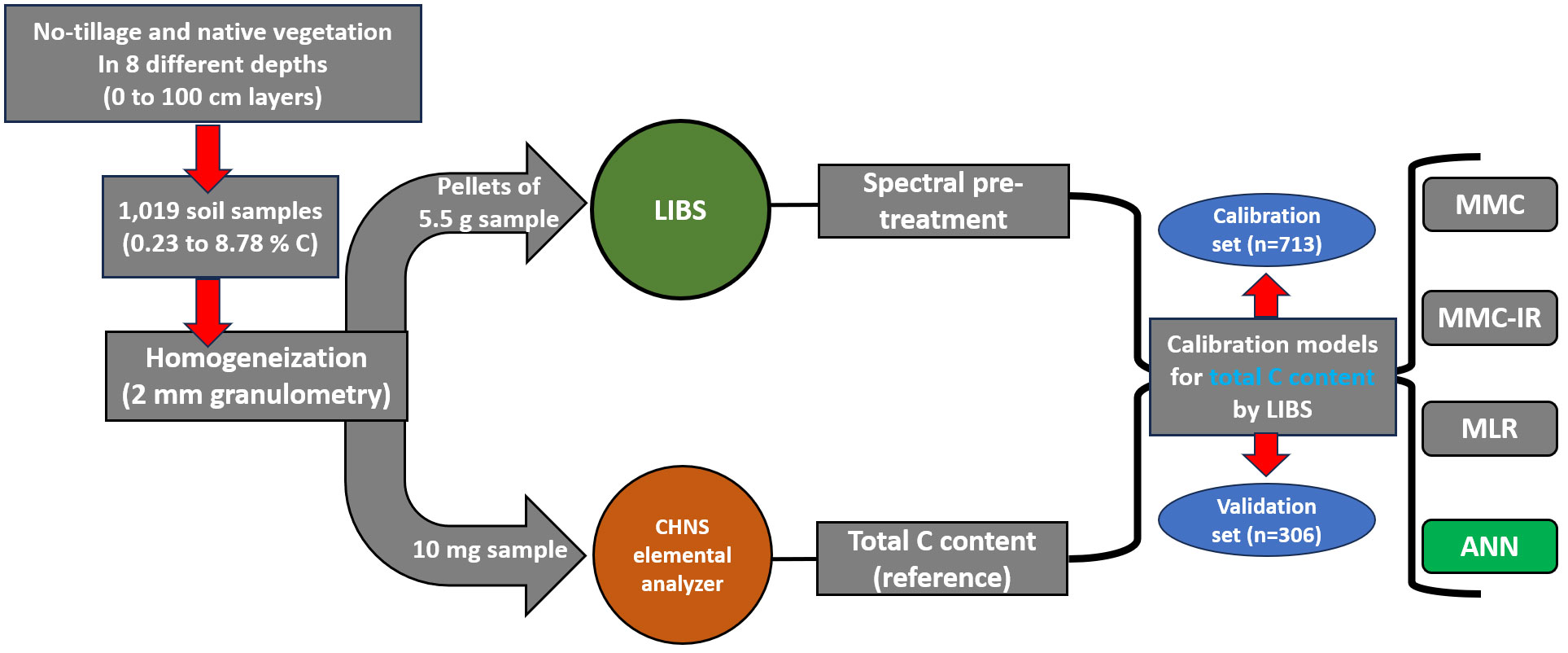
Figure 4 Flowchart of the main steps involved in the methodology developed to determine the total C content in soil samples by LIBS.

3 Results

3.1 Soils texture and color, and statistical parameters of the calibration and validation sets

Using the textural triangle obtained (Figure 5), most of the samples analyzed by LIBS had clay texture (72.5%), followed by sandy clay loam (7.75%), clay loam (6.12%), sandy loam (5.35%), and sandy clay (4.30%). The rest of the samples (3.98% of the samples) were classified into other categories. Soil samples also had different colors, including red (the most predominant), yellow, brown, and gray (Figure 2).

Figure 5

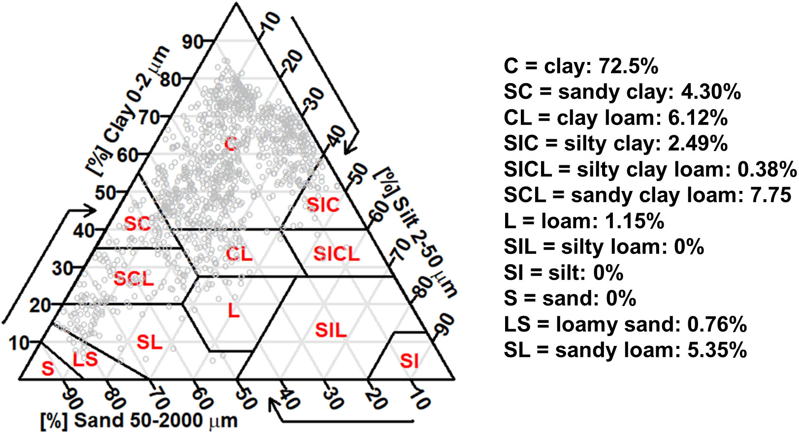
Figure 5 Classification of all soils set by USDA textural triangle.

The calibration and validation sets are made up of soil samples with great variability in total C content and collected at different depths, for both sets (see Supplementary Figure S3. Summary statistics of total C contents at each sampling depth (0 to 100 cm): minimum, maximum, average, standard deviation, and coefficient of variation for calibration sets and validation, in the Supplementary Material).

3.2 Analytical performance parameters of the models

The parameters calculated for each model are shown in Table 1. Using matrix-matching calibration – MMC and MMC - inverse regression, the calculated values of r and R² equal 0.71 and 0.50, respectively. In the MMC–inverse regression model, the RMSEP value (0.67 wt% C) was 1.47-fold lower than that of the traditional MMC (0.99 wt% C).

Table 1

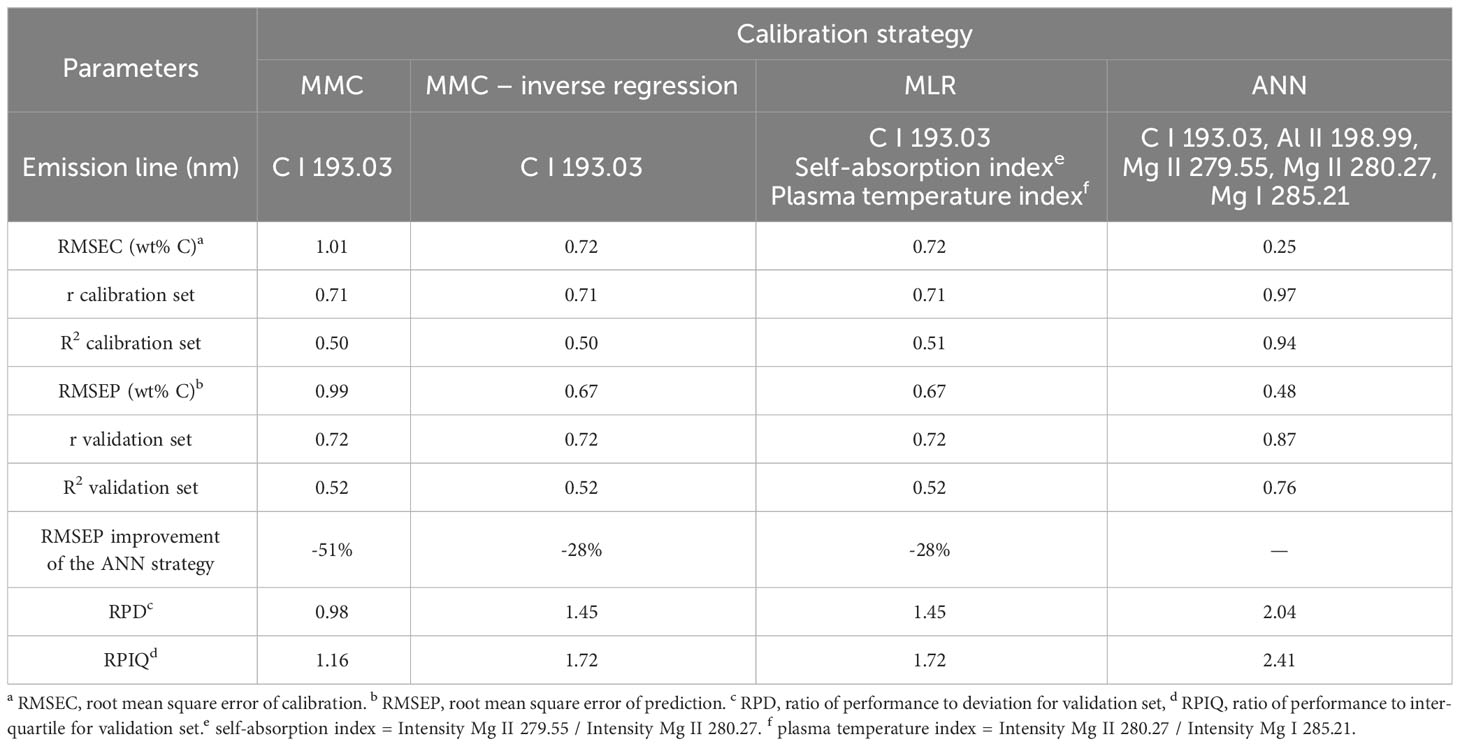
Table 1 Analytical performance parameters of proposed LIBS methods for the determination of total C in soil samples.

For the evaluated multivariate strategies (MLR and ANN), the ANN model showed better predictive ability (RMSEP 0.48 wt% C), with a 1.4-fold lower prediction error when compared to the MLR (RMSEP 0.67 wt% C; Table 1). The best result was obtained using the ANN model with 50 neurons in the hidden layer using the reLU activation function and one neuron in the output layer using a linear function. The training of the ANN model took approximately 4 min, stopping at 4000 epochs with a mean square error (MSE) value of 22.78 wt%. The ANN model resulted in the best correlation coefficient values of the calibration set (0.97) and validation set (0.87) between the C values determined by LIBS versus the reference values obtained by the elemental analyzer, as shown in Figure 6.

Figure 6

Figure 6 Correlation between predicted values (determined by proposed LIBS method using ANN) versus reference values (determined by CHNS elemental analyzer method) for total C contents.

Thus, Table 1 shows the performance gain (in the percentage of RMSEP reduction) of the best-performing model (ANN) compared to the others. Compared with the MMC, MMC-inverse regression, and MLR, the RMSEP (ANN) values were 51%, 28%, and 28% lower, respectively.

The performance of the models was also evaluated based on the magnitude of the calculated RPD and RPIQ values (Table 1). The RPD and RPIQ values were 0.98 and 1.16 for the MMC model, 1.45 and 1.72 for the MMC-inverse regression, 1.45 and 1.72 for the MLR model, and 2.04 and 2.41 for the ANN model, respectively.

3.3 Comparison of total C values obtained by LIBS and CHNS methods

The coefficient of determination (R²) was calculated for the total C contents values, using the LIBS and CHNS reference methods, for the soil samples of the 11 farms (Figure 7). The R² values for each farm (F) were R² = 0.92 (F1), R² = 0.68 (F2), R² = 0.92 (F3), R² = 0.93 (F4), R² = 0.73 (F5), R² = 0.93 (F6), R² = 0.85 (F7), R² = 0.93 (F8), R² = 0.29 (F9), R² = 0.87 (F10), and R² = 0.92 (F11).

Figure 7

Figure 7 Correlation between predicted values (determined by proposed LIBS method) versus reference values (determined by CHNS elemental analyzer method) for total C contents per farm.

4 Discussion

4.1 Variability of texture and color of soil samples: matrix effects in LIBS

Soil samples are geochemically complex samples from an analytical point of view (13, 14, 17). Even considering the same area (farm), the chemical composition (e.g., Fe oxides content, Ca carbonate content, and coarse fragment content), and texture of the soils can show high variability due to the intrinsic characteristics of the geological origin, the agricultural management used, and the collection depth (23).

Due to matrix effects, these characteristics may influence the laser pulse–sample interaction during LIBS analysis. The matrix effects can be exemplified by the fact that two soil samples (red squares) (Figure 8) with the same total C content, 3.19 wt% C, have different emission intensities of the C I 193.03 nm line (11.1 (a.u.) for soil #1 and 7.4 (a.u.) for soil #2) and physical properties (texture). The values of sand, silt, and clay for soil #1 are 33.9%, 27.2%, and 38.9%, and for soil #2 are 59%, 6.7%, and 34.3%, respectively. These effects influence, with different magnitudes, the plasma temperature and acquisition of the analytical signal (intensities of the emission lines) referring to carbon and other elements monitored by the technique (23).

Figure 8

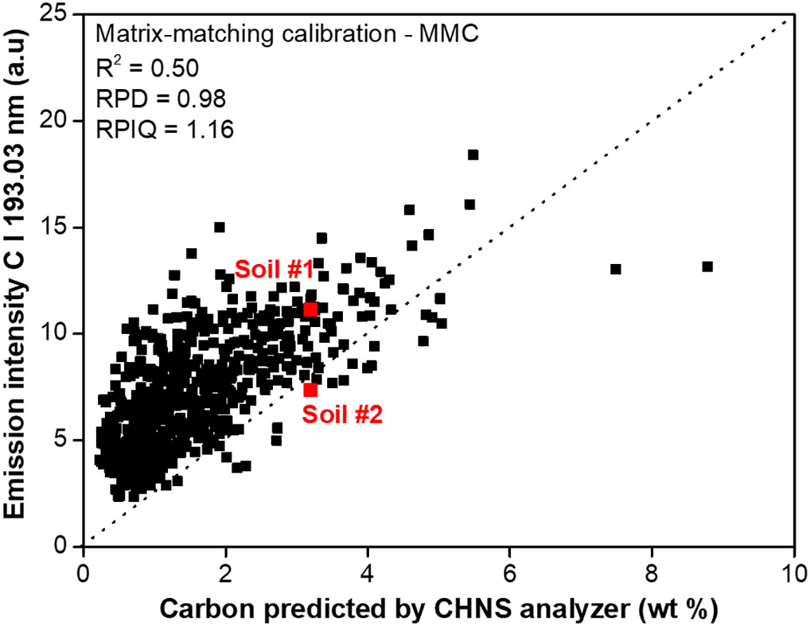
Figure 8 Correlation between the total C content and the emission intensity of the C I 193.03 nm line, for the calibration set (n=713 soils samples), using the MMC strategy.

Standardizing the preparation of soil samples, such as drying, sieving, and the pressure used to prepare pellets, can reduce some physical matrix effects in solid sample analyses. Some studies highlight the importance of collecting and preparing soil samples for examination using spectroscopic techniques, such as NIRS, and how these steps and procedures can influence the accuracy of C determinations in samples (11, 20, 21, 33).

Furthermore, optimizing the instrumental conditions for LIBS, such as spectrometer delay time and laser pulse energy, is necessary to obtain a high signal-to-background ratio of the monitored carbon line. In this way, some physical and chemical matrix effects (or even both) can be reduced.

The soil samples analyzed show different colors (Figure 2). This color difference is due to the intrinsic characteristics of each type of soil, such as chemical composition and granulometry. These factors can also influence LIBS analysis, as variations in the light absorption coefficient of soil samples, thermal conductivity, and fluctuations in the interaction of laser-soil radiation can also reflect the amount of ablated mass, as well as the parameters of the formed plasma (temperature and electron density) (34). Thus, these spectral fluctuations of different magnitudes can still occur even when using 30 laser pulses to analyze each soil sample (as in this study) to minimize sample microheterogeneity and obtain a representative analysis.

4.2 Spectral interferences: reducing chemical matrix effects and the importance of spectral preprocessing

Red-colored soils from these Brazilian tropical and subtropical areas indicate the presence of iron oxides and hydroxides. As is known, Brazilian tropical soils can have a high content of Fe and Al due to their geological origin (22). These two elements are a challenge in monitoring the main observable lines of C by LIBS due to spectral interferences (14, 17, 22), as shown in Figures 3B, C. In Figure 3C, the spectral profile of the C I 247.87 nm line is shown. Observe the strong spectral interference of the Fe I 247.98 nm line in this analyte line, as well as the presence of adjacent lines that overlap in this region. Despite the spectral interference of Al atomic and ionic lines in the C 193.03 nm line and being attenuated by the O₂(g) absorption (when LIBS analyses are done under air atmosphere) (14), this line is more suitable in the proposition of the calibration models (Figure 3B). A strategy used to reduce this spectral interference is the deconvolution of the Al 193.58 nm line. This strategy minimizes the contribution of spectral interference to the intensity of the C I 193.03 nm line. This allows for the accuracy of the determination of C by LIBS.

In this context, it is necessary to evaluate i) spectral pretreatments (from baseline correction, spectral deconvolution to overcome spectral interferences (e.g., Al interference in C I 193.03 nm emission line), ii) better strategies to accurately calculate the area and height of the monitored C emission line, and iii) univariate and multivariate method calibration strategies to reduce these matrix effects.

4.3 Overcoming the physical and chemical matrix effects of soils in LIBS

The quantification models using MMC and MMC-inverse regression allow for compensation for matrix effects since, when using a specific set of soil samples as calibration standards, it is assumed that there is a similarity in the physical-chemical properties of the samples used as a standard and validation set samples (28, 29). However, significant matrix effects were observed (due to the low quality of the modeling obtained, using the MMC strategy, RPD = 0.98, RPIQ = 1.19 and R² = 0.50, Figure 8) and the choice of variables as dependent and independent uses in the least squares regression could significantly influence the predictive capacity of quantification models, as evidenced by the RMSEP values. When using the C emission line as the independent variable (MMC-inverse regression), supposedly without error, the model improved the predictive capacity of the total C concentration in the samples. This may indicate that the error associated with acquiring the analytical signal is smaller than the error associated with determining the total C by the reference technique.

The difference in the texture of the analyzed soils is another factor that may have influenced the laser pulse–sample interaction and, consequently, the RMSEP values calculated by the models. Although the soil samples originated from predominantly clay texture soils, sandy texture samples (such as F10, Figure 5) were also analyzed and used in the calibration and validation sets. Segnini et al. (23) demonstrated that the magnitude of physical (texture) and chemical matrix effects influence the modeling and limits of detection for C in soils using the LIBS method. Thus, in the MMC- and MMC-inverse regression models, matrix effects and the choice of variables (dependent or independent) used in the least squares regression models were the main components influencing the calculated analytical results.

In multivariate strategies (MLR and ANN), using multiple variables correlated to the analyte concentration, sample matrix information, and plasma parameters generated by LIBS can improve the predictive capacity of the models. The MLR model, using indices related to plasma temperature and the possible self-absorption effect, presented an RMSEP value similar to the value obtained by MMC-inverse regression. However, the RMSEP for MLR was 32% lower than that for MMC, contributing to the increased accuracy of C determinations in soil samples.

One of the significant advantages of ANN is the possibility of modeling the interferences and nonlinear signals using several variables that can contribute to reducing matrix effects (28, 35). Thus, the use of variables around the emission lines of the elements (C I 193.03 nm, Al II 198.99, Mg II 279.55 nm, Mg II 280.27 nm, and Mg I 285.21 nm) in ANN modeling makes it possible to predict with reasonable accuracy the C concentration in soil samples analyzed directly by LIBS. As mentioned earlier, the spectral interference of Al atomic and ionic lines on the C I 193.03 nm line can be observed mainly in tropical soils (22). Therefore, the intensity of the Al line correlated to the spectral interference of the analyte and the chemical composition of the sample matrix (tropical soils are rich in aluminosilicates) was used. Magnesium emission lines (associated with minerals) allowed us to obtain chemical information from the soil samples that would help to improve the modeling and, consequently, the accuracy of the predictions of total C.

Nawar and Mouazen (2017) (36) proposed the following groups for RPIQ interpretation: excellent models (RPIQ ≥ 2.5), very good models (2.5 > RPIQ ≥ 2.0), good models (2.0 > RPIQ ≥ 1.7), reasonable models (1.7 > RPIQ ≥ 1.4), and very poor models (RPIQ < 1.4). Thus, a very good model (RPIQ = 2.41) was calculated using the ANN strategy to determine the C content in soils. Using this model for predictions of total C by LIBS, and correlating with the values obtained by the reference method (Figure 7), very good R² values (0.68 ≤ R² ≤ 0.93) were obtained for determinations in the soil samples of 10 of the 11 farms analyzed (with the exception of F9, R² = 0.29; due to possible matrix effects). The possible effects arising from the variability of the sample matrix, specifically related to Fe oxides content, calcium carbonate content, coarse fragment content, and color, can also influence determinations. In future studies, also addressing on-farm research, we intend to determine and evaluate how these contents could directly influence the determinations of total C in soil samples by LIBS.

Considering the calculated RMSEP values (Table 1) for the four models obtained, the predictive capacity of the direct determination of total C in soil samples by LIBS was of the following order: ANN > MLR = MMC-inverse regression > MMC. It can be seen from these values in Table 1 how the accuracy of C determination varies depending on the calibration strategy used (even using the same calibration and validation set for all). Each intrinsic characteristic of the calibration strategy manages to compensate for specific physical and chemical matrix effects and allows determination at different levels of reliability.

The RMSEP values obtained in the determination using the ANN (RMSEP = 0.48 wt% C) and LIBS were slightly higher than the error associated with the C determination by the reference method by the CHNS elemental analyzer, which is approximately 0.30 wt% C (37). This result indicates that LIBS has accuracy comparable to the reference method used but with more analytical advantages, as mentioned earlier.

Some spectroscopic methods of determination of total C in soil samples have been reported in the scientific literature using NIRS and LIBS techniques. Satisfactory prediction error values were obtained using the methods used here. For example, using NIRS, Morgan et al. (2009) (38) reported a RMSEP value of 0.54% C and 0.41% C (n = 164 soils samples) for the field-moist soils and air-dried intact soils scans, respectively. Roudier et al. (2015) (11), using vis-NIRS, obtained an RMSE of 0.38% C (n = 30 cores, 89 spectra). Guedes et al. (2023) (32) recently reported an RMSEP of 0.10% C (n = 48 soil samples) for the analysis of tropical soil samples obtained in long-term field experiments conducted by a research institution using LIBS. Knadel et al. (2017) (18), using the LIBS (RMSEP = 0.50 and 0.85% C, n = 54 soils samples) and vis-NIRS (RMSEP = 0.48 and 1.17% C, n = 54) techniques, obtained good performance parameters, using PLS regression for modeling and two sets of samples for calibration (1-calibration data set based on country-scale data set only, and 2- calibration data set based on country-scale data set spiked with field samples). However, as highlighted by the authors, the LIBS method made it possible to obtain lower prediction errors for soil organic carbon when compared to the vis-NIRS method.

The model proposed in this study (RMSEP of 0.48%) was similar to the previously mentioned studies. However, it is essential to highlight that in the present study, the modeling (n = 713 soil samples) and the verification of the predictive capacity of the LIBS method occurred on a much larger scale (n = 306 soil samples) and used samples with significant variability in total C content, different depths, sampling sites, and biomes. Therefore, the developed model was robust and demonstrated the real ability of the LIBS technique to assist C determination in tropical and subtropical soil samples.

4.4 Evaluation of the advantages and limitations of LIBS and CHNS elemental analyzers in C determination in soils

Figure 9 illustrates the main differences and similarities between the evaluated methods, considering some parameters. The method of using the elemental analyzer by CHNS is consolidated in the scientific literature and routine soil analysis laboratories (10). This method has advantages, highlighting the accuracy of the determinations. However, the limitations include using several consumable materials and more significant cost and analysis time (compared to the LIBS method) (9, 10).

Figure 9

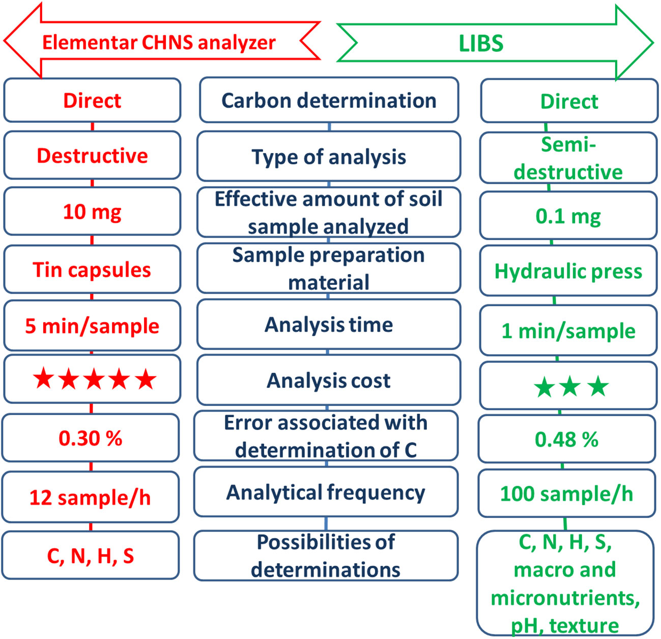
Figure 9 Comparison of soil C determination methods using dry combustion (CHNS elemental analyzer) and LIBS techniques.

Some limitations of the LIBS method still need to be overcome, such as a) increasing the sensitivity of the methods for the determination of analytes at low concentrations and b) the proposition of robust calibration methods that make it possible to efficiently reduce the influence of chemical and physical matrix effects of soil samples, and consequently further improve the accuracy of determinations (14).

However, LIBS as a new analytical tool for soil C determination has several advantages, such as (a) a smaller amount of analyzed sample needed, (b) high analytical frequency, (c) accuracy comparable to the reference method (as demonstrated in this work), and (d) lower analysis cost. Different from the CHNS elemental analyzer, LIBS multielemental analysis allows co-benefits in the analysis because, from the emission spectrum of the sample obtained, it is possible, through preestablished quantitative models, to determine i) macro- and micronutrients (used in the evaluation of the fertility of the soil) (12), ii) prediction of soil texture (39), and iii) pH (40) and other attributes of the analyzed soil sample.

5 Conclusion

The study reveals that the proposed LIBS method offers to agricultural producers a viable means of measuring total carbon in soil samples with reasonable accuracy. The magnitude of the matrix effects, influenced by the diverse physicochemical properties of soil samples (despite no data available on Fe oxides content, Ca carbonate content, and Coarse fragment content), was successfully reduced through the intrinsic characteristics of the evaluated calibration strategies, leading to improved predictions of total C in tropical soils. Notably, the ANN model yielded the lowest RMSEP value (0.48 wt% C), an acceptable figure compared to the elemental analyzer (0.30 wt% C) – the reference method. LIBS is a practical, rapid, and cost-efficient analytical technique for directly quantifying C in tropical and subtropical soil samples extensive on-farm research. While the proposed LIBS method and the reference CHNS elemental analyzer method have their respective strengths and weaknesses, LIBS demonstrates superior performance in analytical frequency (100 samples h^-1), cost-effectiveness, and the potential for simultaneous determination of other soil attributes.

Data availability statement

The original contributions presented in the study are included in the article/Supplementary Material. Further inquiries can be directed to the corresponding author.

Author contributions

DB: Conceptualization, Methodology, Investigation, Validation, Data curation, Formal analysis, Writing - original draft. WG: Conceptualization, Methodology, Investigation, Validation, Data curation, Formal analysis, Writing - original draft. VF: Conceptualization, Methodology, Investigation, Validation, Data curation, Formal analysis, Writing - original draft. FS: Methodology, Validation, Formal analysis. MT: Methodology, Validation, Formal analysis. PV-B: Conceptualization, Methodology, Investigation, Validation, Data curation, Formal analysis, Writing - original draft. LM-N: Conceptualization, Resources, Writing - review & editing, Supervision, Project leader, Funding acquisition. DM: Conceptualization, Resources, Writing - review & editing, Supervision, Funding acquisition. All authors contributed to the article and approved the submitted version.

Funding

The author(s) declare financial support was received for the research, authorship, and/or publication of this article. Foundation Arthur Bernardes- FUNARBE, Brazilian Agency (Project number: 6823), a joint project between Embrapa and Bayer Corporation (Brazilian branch). National Council of Scientific and Technological Development- CNPq (Brazilian Agency, National Laboratory of Agri-Photonics- LANAF, Project number: 440226/2021-0). Embrapa System of Management- SEG - “Balance and carbon footprint in the production of soybean, maize and sugar-cane: metrics, tools and protocols to tropical and subtropical areas of Brazilian territory”, SEG: 20.22.00.118.00.00.

Acknowledgments

The authors are grateful to the FUNARBE for fellowships and Bayer S.A. for financial support. We also thank Embrapa Instrumentation, LANAF, and CNPq for the laboratory infrastructure for this research development.

Conflict of interest

The authors declare that the research was conducted in the absence of any commercial or financial relationships that could be construed as a potential conflict of interest.

This study received funding from Bayer Company Brazilian branch through a Public-Private Partnership agreement. The contract was signed according to Brazilian laws. The company financially supported the execution of activities, such as CHN analysis, LIBS measurements, and data treatments. However, no scientific contribution was made by Bayer’s members.

The authors DMBPM and LM-N declared that they were an editorial board member of Frontiers, at the time of submission. This had no impact on the peer review process and the final decision.

Publisher’s note

All claims expressed in this article are solely those of the authors and do not necessarily represent those of their affiliated organizations, or those of the publisher, the editors and the reviewers. Any product that may be evaluated in this article, or claim that may be made by its manufacturer, is not guaranteed or endorsed by the publisher.

Supplementary material

The Supplementary Material for this article can be found online at: https://www.frontiersin.org/articles/10.3389/fsoil.2023.1242647/full#supplementary-material

References

1. Tadini AM, Xavier AAP, Milori DMBP, Oliveira PPA, Pezzopane JR, Bernardi ACC, et al. Evaluation of soil organic matter from integrated production systems using laser-induced fluorescence spectroscopy. Soil Tillage Res (2021) 211:105001. doi: 10.1016/j.still.2021.105001

CrossRef Full Text | Google Scholar

2. Bayer C, Martin-Neto L, Mielniczuk J, Pavinato A, Dieckow J. Carbon sequestration in two Brazilian Cerrado soils under no-till. Soil Tillage Res (2006) 86:237–45. doi: 10.1016/j.still.2005.02.023

CrossRef Full Text | Google Scholar

3. Sá JCM, Lal R, Cerri CC, Lorenz K, Hungria M, Carvalho PCF. Low-carbon agriculture in South America to mitigate global climate change and advance food security. Environ Int (2017) 98:102–12. doi: 10.1016/j.envint.2016.10.020

PubMed Abstract | CrossRef Full Text | Google Scholar

4. Bieluczyk W, Piccolo MC, Pereira MG, Moraes MT, Soltangheisi A, Bernardi ACC, et al. Integrated farming systems influence soil organic matter dynamics in southeastern Brazil. Geoderma (2020) 371:114368. doi: 10.1016/j.geoderma.2020.114368

CrossRef Full Text | Google Scholar

5. Nicoloso RS, Rice CW. Intensification of no-till agricultural systems: an opportunity for carbon sequestration. Soil Sci Soc Am J (2021) 85:1395–409. doi: 10.1002/saj2.20260

CrossRef Full Text | Google Scholar

6. Ferreira AO, Amado TJC, Rice CW, Gonçalves DRP, Diaz DAR. Comparing on-farm and long-term research experiments on soil carbon recovery by conservation agriculture in Southern Brazil. Land Degrad Dev (2021) 32:1–12. doi: 10.1002/ldr.4015

CrossRef Full Text | Google Scholar

7. Brammer TA, Bennett DE. Arriving at a natural solution: Bundling credits to access rangeland carbon markets. Rangelands (2022) 44(4):281–90. doi: 10.1016/j.rala.2022.04.001

CrossRef Full Text | Google Scholar

8. The international "4 per 1000" initiative. Available at: https://4p1000.org/?lang=en (Accessed May 08, 2023).

Google Scholar

9. Nayak AK, Rahman MM, Naidu R, Dhal B, Swain CK, Nayak AD, et al. Current and emerging methodologies for estimating carbon sequestration in agricultural soils: a review. Sci Total Environ (2019) 665:890–912. doi: 10.1016/j.scitotenv.2019.02.125

PubMed Abstract | CrossRef Full Text | Google Scholar

10. Chatterjee A, Lal R, Wielopolski L, Martin MZ, Ebinger MH. Evaluation of different soil carbon determination methods. Crit Rev Plant Sci (2009) 28:164–78. doi: 10.1080/07352680902776556

CrossRef Full Text | Google Scholar

11. Roudier P, Hedley CB, Ross CW. Prediction of volumetric soil organic carbon from field-moist intact soil cores. Eur J Soil Sci (2015) 66:651–60. doi: 10.1111/ejss.12259

CrossRef Full Text | Google Scholar

12. Tavares TR, Mouazen AM, Nunes LC, Santos FR, Melquiades FL, Silva TR, et al. Laser-induced breakdown spectroscopy (LIBS) for tropical soil fertility analysis. Soil Tillage Res (2022) 216:105250. doi: 10.1016/j.still.2021.105250

CrossRef Full Text | Google Scholar

13. Villas-Boas PR, Franco MA, Martin-Neto L, Gollany H, Milori DMBP. Applications of laser-induced breakdown spectroscopy for soil analysis, part I: review of fundamentals and chemical and physical properties. Eur J Soil Sci (2020) 71:789–804. doi: 10.1111/ejss.12888

CrossRef Full Text | Google Scholar

14. Villas-Boas PR, Franco MA, Martin-Neto L, Gollany H, Milori DMBP. Applications of laser-induced breakdown spectroscopy for soil characterization, part II: review of elemental analysis and soil classification. Eur J Soil Sci (2020) 71:805–18. doi: 10.1111/ejss.12889

CrossRef Full Text | Google Scholar

15. Cremers DA, Radziemski LJ. History and fundamentals of LIBS. In: Miziolek AW, Palleschi V, Schechter I, editors. Laser-Induced Breakdown Spectroscopy. New York: Cambridge University Press (2006).

Google Scholar

16. Verra. VCS Methodology- VM0042- Methodology for improved agricultural land management, Version 2.0, 30 May 2023, Sectoral Scope 14. Available at: https://verra.org/wp-content/uploads/2023/05/VM0042-Improved-ALM-v2.0.pdf (Accessed September 12, 2023).

Google Scholar

17. Senesi GS, Senesi N. Laser-induced breakdown spectroscopy (LIBS) to measure quantitatively soil carbon with emphasis on soil organic carbon. A review Anal Chim Acta (2016) 938:7–17. doi: 10.1016/j.aca.2016.07.039

CrossRef Full Text | Google Scholar

18. Knadel M, Gislum R, Hermansen C, Peng Y, Moldrup P, de Jonge LW, et al. Comparing predictive ability of laser-induced breakdown spectroscopy to visible near-infrared spectroscopy for soil property determination. Biosyst Eng (2017) 156:157–72. doi: 10.1016/j.biosystemseng.2017.01.007

CrossRef Full Text | Google Scholar

19. Brown DJ. Using a global VNIR soil-spectral library for local soil characterization and landscape modeling in a 2nd-order Uganda watershed. Geoderma (2007) 140(4):444–53. doi: 10.1016/j.geoderma.2007.04.021

CrossRef Full Text | Google Scholar

20. Brunet D, Barthès BG, Chotte J, Feller C. Determination of carbon and nitrogen contents in Alfisols, Oxisols and Ultisols from Africa and Brazil using NIRS analysis: effects of sample grinding and set heterogeneity. Geoderma (2007) 139:106–17. doi: 10.1016/j.geoderma.2007.01.007

CrossRef Full Text | Google Scholar

21. Barthès BG, Brunet D, Ferrer H, Jean-Luc Chotte J, Feller C. Determination of total carbon and nitrogen content in a range of tropical soils using near infrared spectroscopy: influence of replication and sample grinding and drying. J Near Infrared Spectrosc (2006) 14:341–8. doi: 10.1255/jnirs.686

CrossRef Full Text | Google Scholar

22. Nicolodelli G, Marangoni BS, Cabral JS, Villas-Boas PR, Senesi GS, dos Santos CH, et al. Quantification of total carbon in soil using laser-induced breakdown spectroscopy: a method to correct interference lines. Appl Opt (2014) 53:2170–6. doi: 10.1364/AO.53.002170

PubMed Abstract | CrossRef Full Text | Google Scholar

23. Segnini A, Xavier AAP, Otaviani-Junior PL, Ferreira EC, Watanabe AM, Sperança MA, et al. Physical and chemical matrix effects in soil carbon quantification using laser-induced breakdown spectroscopy. Am J Anal Chem (2014) 5:722–9. doi: 10.4236/ajac.2014.511080

CrossRef Full Text | Google Scholar

24. Ebinger MH, Norfleet ML, Breshears DD, Cremers DA, Ferris MJ, Unkefer PJ, et al. Extending the applicability of laser-induced breakdown spectroscopy for total soil carbon measurement. Soil Sci Soc Am J (2003) 67:1616–9. doi: 10.2136/sssaj2003.1616

CrossRef Full Text | Google Scholar

25. Martin MZ, Labbé N, André N, Wullschleger SD, Harris RD, Ebinger MH. Novel multivariate analysis for soil carbon measurements using laser-induced breakdown spectroscopy. Soil Sci Soc Am J (2010) 74:87–93. doi: 10.2136/sssaj2009.0102

CrossRef Full Text | Google Scholar

26. Teixeira PC, Donagemma GK, Fontana A, Teixeira WG eds. Manual de métodos de análise de solo, Empresa Brasileira de Pesquisa Agropecuária (Embrapa). 3rd edition. Brasília, Brazil: Embrapa (2017) p. 66–75, ISBN: ISBN 978-85-7035-771-7.

Google Scholar

27. Natural Resources Conservation Service. U.S. Department of Agriculture. Available at: https://www.nrcs.usda.gov/resources/education-and-teaching-materials/soil-texture-calculator (Accessed May 08, 2023).

Google Scholar

28. Marangoni BS, Silva KSG, Nicolodelli G, Senesi GS, Cabral JS, Villas-Boas PR, et al. Phosphorus quantification in fertilizers using laser induced breakdown spectroscopy (LIBS): a methodology of analysis to correct physical matrix effects. Anal Methods (2016) 8:78–82. doi: 10.1039/c5ay01615k

CrossRef Full Text | Google Scholar

29. Costa VC, Babos DV, Castro JP, Andrade DF, Gamela RR, MaChado RC, et al. Calibration strategies applied to laser-induced breakdown spectroscopy: a critical review of advances and challenges. J Braz Chem Soc (2020) 31:2439–51. doi: 10.21577/0103-5053.20200175

CrossRef Full Text | Google Scholar

30. Duponchel L, Bousquet B, Pelascinic F, Motto-Ros V. Should we prefer inverse models in quantitative LIBS analysis? J. Anal At Spectrom (2020) 35:794–803. doi: 10.1039/C9JA00435A

CrossRef Full Text | Google Scholar

31. Yao S, Shen Y, Yin K, Pan G, Lu J. Rapidly measuring unburned carbon in fly ash using molecular CN by laser-induced breakdown spectroscopy. Energy Fuels (2015) 29:1257–63. doi: 10.1021/ef502174q

CrossRef Full Text | Google Scholar

32. Guedes WN, Babos DV, Costa VC, Morais CP, Freitas VS, Stenio K, et al. Evaluation of univariate and multivariate calibration strategies for the direct determination of total carbon in soils by laser-induced breakdown spectroscopy: tutorial. J Opt Soc Am B (2023) 40:1319–30. doi: 10.1364/JOSAB.482644

CrossRef Full Text | Google Scholar

33. Cardinael R, Chevallier T, Barthès BG, Saby NPA, Parent T, Dupraz C, et al. Impact of alley cropping agroforestry on stocks, forms and spatial distribution of soil organic carbon - A case study in a Mediterranean context. Geoderma (2015) 259–260:288–99. doi: 10.1016/j.geoderma.2015.06.015

CrossRef Full Text | Google Scholar

34. Takahashi T, Thornton B. Quantitative methods for compensation of matrix effects and self-absorption in laser induced breakdown spectroscopy signals of solids. Spectrochim Acta B (2017) 138:31–42. doi: 10.1016/j.sab.2017.09.010

CrossRef Full Text | Google Scholar

35. Guedes WN, dos Santos LJ, Fillitti ÉR, Pereira FMV. Sugarcane stalk content prediction in the presence of a solid impurity using an artificial intelligence method focused on sugar manufacturing. Food Anal Methods (2020) 13:140–4. doi: 10.1007/s12161-019-01551-2

CrossRef Full Text | Google Scholar

36. Nawar S, Mouazen AM. Predictive performance of mobile vis-near infrared spectroscopy for key soil properties at different geographical scales by using spiking and data mining techniques. Catena (2017) 151:118–29. doi: 10.1016/j.catena.2016.12.014

CrossRef Full Text | Google Scholar

37. Perkin Elmer.Available at: https://www.perkinelmer.com.br/product/2400-chns-o-series-ii-system-100v-n2410650 (Accessed June 08, 2022).

Google Scholar

38. Morgan CLS, Waiser TH, Brown DJ, Hallmark CT. Simulated in situ characterization of soil organic and inorganic carbon with visible near-infrared diffuse reflectance spectroscopy. Geoderma (2009) 151:249–56. doi: 10.1016/j.geoderma.2009.04.010

CrossRef Full Text | Google Scholar

39. Villas-Boas PR, Romano RA, Franco MAM, Ferreira EC, Ferreira EJ, Crestana S, et al. Laser-induced breakdown spectroscopy to determine soil texture: a fast analytical technique. Geoderma (2016) 263:195–202. doi: 10.1016/j.geoderma.2015.09.018

CrossRef Full Text | Google Scholar

40. Ferreira EC, Gomes Neto JA, Milori DM, Ferreira EJ, Anzano JM. Laser-induced breakdown spectroscopy: extending its application to soil pH measurements. Spectrochim Acta B (2015) 110:96–9. doi: 10.1016/j.sab.2015.06.002

CrossRef Full Text | Google Scholar