Linking electromagnetic induction data to soil properties at field scale aided by neural network clustering

1 Introduction

Soil is a fundamental natural resource that plays a pivotal role in sustaining life on Earth (1, 2), acting as the foundation for 95% of food production and 25% of all biodiversity (3). It forms one of the three components of environmental quality, alongside air and water quality (4) and is included in several Sustainable Development Goals (5). Soil physical properties significantly impact agricultural productivity and environmental health (6, 7). An accurate understanding of the spatial distribution of soil physical properties is essential at national and local levels to make informed decisions regarding land use planning, agricultural practices, and environmental conservation (8, 9).

Static soil properties (e.g., soil texture, mineral composition, bulk density, and porosity), which relate to a soil’s capability to function (7), remain generally constant over time and are not significantly influenced by short-term environmental conditions (10). In contrast, dynamic soil properties (e. g., soil moisture, salinity and temperature) exhibit temporal variability and are influenced by short-term environmental factors. These properties have a significant impact on soil condition (i.e., fertility, nutrient cycling, and carbon sequestration (10), making them essential to consider in agricultural practices and ecosystem management (11). Static properties provide a baseline characterization of soil while dynamic properties offer insights into its responsiveness to varying environmental conditions (4, 7). At national policy level, mapping both static and dynamic soil physical properties is paramount for efficient agricultural planning and policy development (2, 12).

At field scale, precision agriculture (13), an emerging practice that utilizes site-specific information for decision-making, benefits from accurate soil property data (14). Farmers can optimize input, such as irrigation and fertilization (15), leading to improved resource efficiency and reduced costs. Furthermore, understanding soil property distribution allows farmers to assess the risks associated with various agricultural practices, making informed choices to avoid soil degradation and ensure long-term productivity and sustainability (16).

Traditional mapping of soil properties (8, 17) involves labor-intensive field surveys and sampling campaigns, where soil samples are collected at points within a study area, before undergoing laboratory analysis to determine static and dynamic properties. These data are then interpolated to create soil maps, providing insights into the spatial distribution of soil properties (9). While offering valuable information, traditional methods are limited in spatial and temporal coverage and are time-consuming and costly. Non-invasive geophysical methods, such as electromagnetic induction (EMI), offer efficient broader coverage and high-resolution mapping capabilities for soil properties (18–21). Multi-coil and/or multi-frequency EMI instruments allow several depths to be sampled simultaneously and can be interpreted to provide the underlying distribution of electrical conductivity (mS/m) (19). At field scale, EMI measurements have been used to map soil texture (22), soil cation exchange capacity (23, 24), soil moisture (25), and soil salinity (26, 27). EMI data have also been used to guide field sample campaigns by clustering (grouping) similar EMI data into management zones, which represent areas of similar soil properties (22, 28) or anthropogenic effects, such as compaction (29).

There are several challenges in utilizing EMI data for soil property mapping. Firstly, the measurements, known as the apparent electrical conductivity (ECa), are the result of a complex combination of several soil physical properties (18). Secondly, the apparent electrical conductivity provides an average, or bulk, measurement for the depth of soil through which the electromagnetic field has passed (30). The depth of penetration is dependent on the frequency of the applied alternating EM field, the separation of the transmitter and receiver coils, and the true electrical conductivity of the medium (31). ECa data can be inverted to produce a model of true electrical conductivity (ECt) distribution of the subsurface (32, 33). The ECt in soil can be regarded as a combination of the conductivity associated with electrical current flow in interconnected pore space and the surface conductivity associated with current flow at clay grain fluid interfaces (34). The ECt is needed for linking traditionally sampled data to modern pedophysical models (35) which can use electrical conductivity to predict soil physical properties.

Non-linear iterative inversion is a computational method that refines ECt models by iteratively adjusting inversion parameters to minimize the difference between observed ECa and predicted ECa. Inversion usually requires an estimation of the starting ECt model. (24, 32). Specifically, knowledge of an initial ECt model can significantly improve the results (36). Often a single initial conductivity model is defined and used at every datapoint across a site. Given the importance of this initial model, this may not be an optimum approach for an inversion, so it is proposed here that a spatially variable initial model is explored prior to inversion.

This study presents a technique to improve the transformation of ECa, to a property (ECt) of the soil column beneath an EMI instrument via a non-linear iterative inversion algorithm. It provides an objective method to determine a spatially variable initial electrical conductivity model to guide an inversion of measured ECa across a field site. The methodology utilizes a machine learning clustering algorithm alongside inversion software to produce the highest appropriate number of initial models for a study site. These initial models are then used as input to Q3D inversions to produce true conductivity distribution on field sites in Germany and Ireland, where soil samples have already been taken. These inversions are compared to results from the traditional approach in which a single, uniform, initial model for a site is used within the inversion. The methodology may allow for a Quasi-3D (Q3D) inversion of measured EMI data on field sites where little or no ground sample data exist, or where a ground sampling campaign is planned. This study also proposes that an EMI survey has the potential to be an initial tool of a soil surveyor, performed prior to and used to guide traditional soil sampling campaigns.

2 Materials and methods

2.1 Electromagnetic induction

EMI estimates the electrical conductivity of the subsurface by inducing alternating electromagnetic fields using a transmitting (Tx) coil (19). This primary field induces electrical currents in the subsurface, which then generate secondary electromagnetic fields (Figure 1). These secondary fields are then detected by a receiving (Rx) coil and the ratio of the primary to secondary field allows for a value of electrical conductivity to be estimated (37, 38). The depth of investigation depend on the frequency of the alternating current in the transmitting coil (1 – 100 kHz), the orientation of the Tx and Rx coils (vertical, horizontal, coplanar), the separation of the Tx and Rx and the electrical conductivity of the subsurface (19, 37).

Figure 1

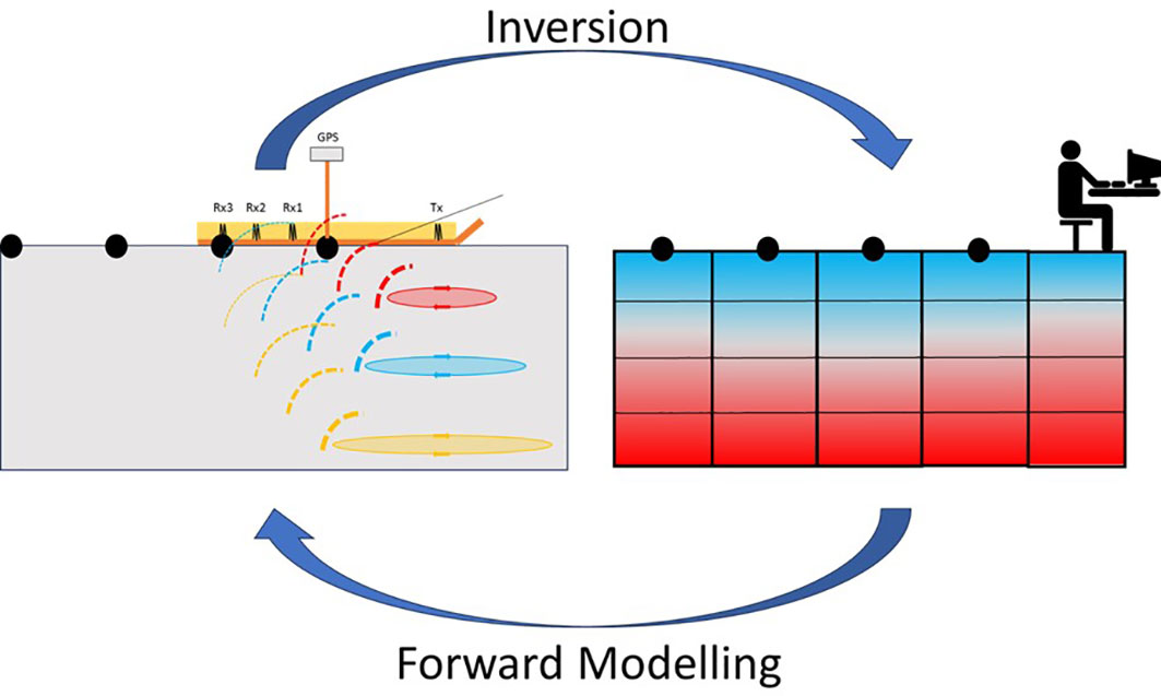
Figure 1 Conceptual diagram for the relationship between acquired EMI data (ECa) and the inverted theoretical response (ECt). Left: Field acquisition using an instrument with 3 coil separations. Black dots indicate the measurement location of the instrument at the surface, colored circles indicate induced current with approximate depth of investigation and resolution for each coil separation. Dashed colors indicate sections of induced secondary magnetic field lines, which are detected at each Rx. Right: Model of electrical conductivity of subsurface divided into layers with each color representing an ECt value.

In this study a CMD Mini-Explorer Special Edition (39) was used on a site in Germany and a CMD Mini-Explorer 6L (39) was used in a site in Ireland. These instruments have a constant Tx frequency and six Rx coils at various separations, allowing for six simultaneous EMI measurements. The instruments differ only in the coil separations. Both instruments were operated in “Hi” mode, or horizontal coplanar coil orientation, allowing for a maximum depth of investigation of ~ 2 - 3 m, with the effective depth of a measurement ~ 1.5 times the coil separation (37). As the EMI instruments and acquisition techniques were very similar on both sites, an identical processing flow was applied to both study sites (Figure 2). This included (where necessary) the correction of GPS antenna location to the instrument center, resampling to 1 Hz spatial sampling frequency, averaging of duplicate spatial samples, correction for the presence of a sled, removal of large (> 1 mS/m) variations between measurements, application of a histogram filter (33), a Principal Component Analysis filter (40) and a temperature correction to 25°C (as per Brogi et al. (22)), to remove the effect of temperature differences between surveys. Measured data, with GPS accuracy < 1 m, were then interpolated to a 1 m x 1 m grid using default parameters in the bSpline interpolation in QGIS v3.20.

Figure 2

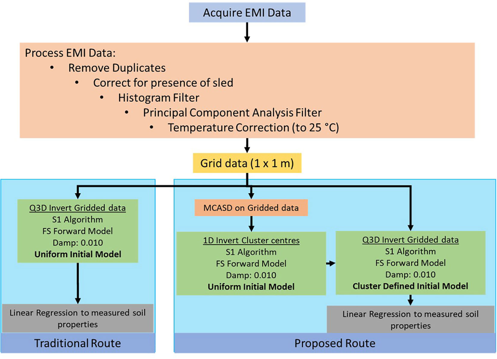
Figure 2 Workflow diagram of methodology applied in this study showing additional steps to achieve data derived initial models for use in inversion.

2.2 Forward modelling and inversion of EMI data

Forward modelling refers to a mathematical process to convert a one-dimensional (1D) layered model of ECt to ECa, the data acquired by an EMI instrument (Figure 1) at the surface of this model. The Maxwell Equations (38) can be used to solve the non-linear 1D forward problem without any restrictions, and with the advent of modern computers can be easily and quickly applied to EMI data (41). Inversion is a mathematical process that translates measured ECa data into a 1D subsurface model of ECt. It involves creating a hypothetical 1D layered subsurface model (Figure 1), then forward modelling to simulate ECa, measured at the instrument at a known height above the ground surface. The process is iterative and uses regularization techniques to refine the model, aiming to minimize the difference between observed ECa and predicted ECa. Typically, an inversion and forward modelling is carried out at a single datapoint at a time before moving on to the next, thereby building a 2D/3D model from a series of EMI datapoints acquired across a site. Several inversion algorithms have been developed (42, 43) to include lateral or spatial constraints during inversion to ensure geological consistency between surrounding 1D models. The technique is known as Quasi-2D/3D (Q2D/Q3D) inversion as it still relies on a 1D forward model for each data point.

An important factor in the inversion process is the choice of an initial ECt model. Traditionally this is a 1D model with a starting conductivity value, which can be a uniform half-space (26) or a representative layered vertical distribution of electrical conductivity (24). In this study, the computation of all models, including initial models and final theoretical responses, is based upon 20 layers, each with a thickness of 0.1 m.

EM4Soil V4.4 (44), a software package for 1D, Q2D and Q3D inversions, is used to invert EMI data using a nonlinear, smoothness-constrained inversion algorithm (S1) and Occam regularization (45). The full solution (FS) of the Maxwell Equations is used to calculate the model response to compare with the ECa. The dampening factor is λ = 0.01 which allows for sharp changes in the vertical distribution of ECt.

2.3 Self-organizing maps clustering

The grouping together of statistically similar multi-dimensional data vectors is often referred to as clustering or classification (46). A data vector is considered as all data located at a single spatial coordinate (47, 48). This study makes use of an unsupervised machine learning classification technique known as Self-Organizing Maps (SOM) (49). Unsupervised classification differs from supervised classification in that there is no requirement for a priori knowledge. Data vectors are grouped based on similarity, which is assumed here to be due to the similar subsurface properties being sensed.

SOM is a centroid based clustering technique, similar to K-Means (50), where each data vector is assigned to a single numerical cluster. K-Means employs a metric consisting of the minimum distance (in the data space) between a data vector and a cluster center to assign each data vector to a numerical cluster. SOM takes advantage of modern neural network machine learning (51) to assess the similarity of data vectors. This cluster center, with similar dimensions to the input data vectors, is representative of all the data assigned to a particular cluster.

The data vectors input to the cluster method are the measured ECa, resulting in a data vector per measurement location, containing as many layers as coil separations (e.g., 6). The aim of clustering EMI data in this study is to firstly divide the study sites into different spatial zones, each of which can be represented by a single EMI data vector, the cluster center. These cluster centers can then act as input to 1D inversion in EM4Soil, producing cluster specific initial model, which can be used as input to a Q3D inversion (Figure 2). Clustering was performed in MATLAB v2023a.

A challenge in any cluster analysis is determining the appropriate number of clusters that can be used to represent a dataset (52, 53). This study uses the Multi-Cluster Average Standard Deviation (MCASD) stability metric which has successfully been applied to airborne geophysical data (48), and ground EMI data (29) similar to this study. This metric assumes that an appropriate number of clusters for a dataset is any at which the cluster center values do not vary significantly when the clustering algorithm is run multiple times. In this study MCASD analysis was tested with a maximum of 12 clusters, with 100 attempts per cluster, to calculate MCASD stability metrics, which are illustrated in Figure 3. The number of clusters and attempts were chosen based on achieving MCASD stability statistics.

Figure 3

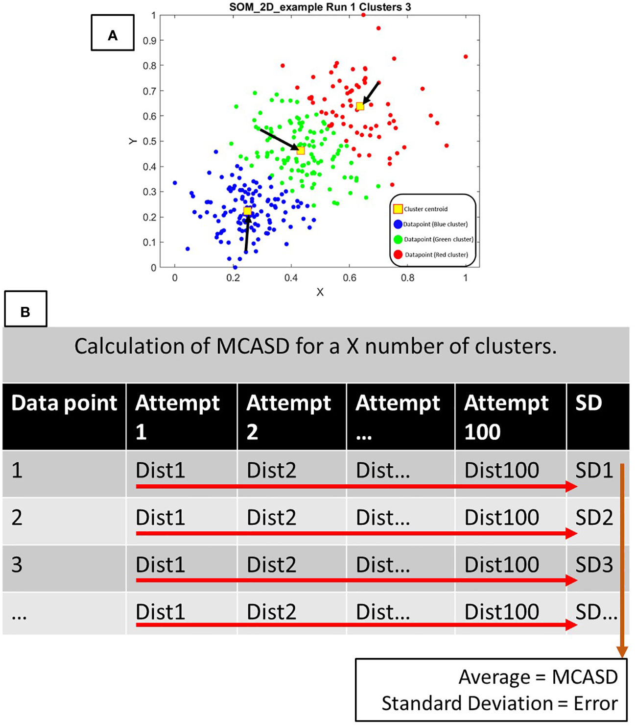
Figure 3 Conceptualization of MCASD. For each datapoint the Euclidean distance in the dataspace between the data vector and the cluster center is calculated and stored for each clustering attempt. After all attempts, a standard deviation (SD) of the distances is calculated. This SD is then averaged for all data points giving the MCASD metric. A SD is calculated to supplement the MCASD metric in the form of a range (error) of this stability across all data vectors. (A) Synthetically generated 2D data showing results after Attempt 1 of a 3-cluster solution. Data vectors are colored based on cluster assignment. Black arrows indicate the Euclidean distance. (B) A visualization of data organization when calculating MCASD metrics. Each row of the table represents a data vector, and each column represents an attempt.

Upon completion of MCASD analysis, the highest number of clusters with a low MCASD metric is selected, as this represents the maximum resolution of the spatial variability that can be obtained through clustering (48).

2.4 Sites

2.4.1 Selhausen, Germany

This site is located near Selhausen, Germany, in the Rur Catchment, ~ 40 km west of Cologne (50°51′56″N 6°27′03″E). The site is part of an agricultural area in which different crops are grown in rotation. These are winter wheat, barley, and sugar beet, with occasional growing of potato, maize, oilseed rape and oats (Figure 4A). The dominant soil groups in the area are cambisols, luvisols, planosols and stagnosols (54). The climatic conditions include mean annual precipitation of 715 mm and annual temperature of 10.2°C. Soil temperature is measured near the investigated site.

Figure 4

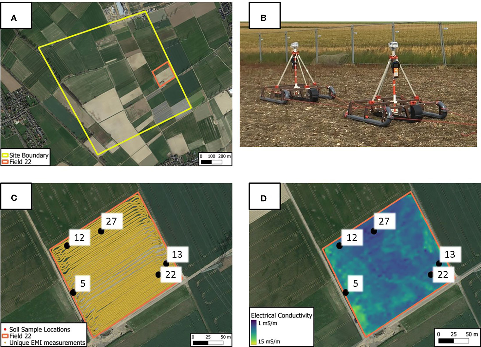
Figure 4 Site description - Germany. (A) Outline of site and study field, (B) EMI set up, (C) EMI measurement locations in Field 22 with soil sample locations, (D) Processed electrical conductivity data (0.5 m coil separation), gridded to 1 m x 1 m with soil sample locations.

Two instruments were used to acquire EMI data, a CMD Mini-Explorer (39) and a prototype CMD Mini Explorer Special edition (Figure 4B). The instruments were towed on GPS equipped plastic sleds in tandem behind a quad bike, with ~ 4 m distance between the first sled and the quad bike and ~ 2 m between the sleds. An average speed of 5 – 7 km/h was maintained, with an inline spatial sampling frequency of 5 Hz, giving an inline spacing of ~ 0.5 m, and a crossline distance of ~ 2 – 2.5 m (Figure 4C). The ECa maps acquired over this site were used by Brogi et al. (22) to subdivide it into soil classes using semi-automatic supervised learning. These classified maps have subsequently been used to inform agroecosystem modelling of crop yield (55). In the study presented, only the data from the CMD Mini-Explorer Special edition was used, as the instrument and measurement configuration are very similar to that used on the second site in Ireland. This instrument has 6 receiver coils with separations of 0.35, 0.50, 0.71, 0.97, 1.35, 1.8 m.

Field 22 (F22) was selected to demonstrate the proposed methodology. This field is part of a local geomorphological feature named Upper Terrace with loess soils of various thickness found above highly compacted sand and gravel that results in the spatial patterns in ECa (22). Data from F22 were acquired on 24^th August 2016. Additionally, 5 ground sample locations (Figure 4; Table 1) were collected in February 2017, the locations of which were guided by the results of semi-automatic classification of the ECa data. After data processing 27,445 EMI measurement locations were gridded to a 1 x 1 m regular grid (Figure 4D). All six EMI coil measurements were processed (Section 2.1) and used for clustering and inversion.

Table 1

Table 1 Soil physical properties for Field 22.

2.4.2 Co. Tipperary, Ireland

This site is a field from a dairy farm (Figure 5A) in Co. Tipperary, Ireland (50°51′56″N 6°27′03″E) growing grass for grazing cattle and fodder. The farm is part of the Heavy Soil Program operated by the Irish Agricultural and Food Agency (56). The main soil groups are typical surface water gley, typical ground water gley, typical luvisol, brown earth and humic surface water gley (57). There is a mean annual precipitation of 980 mm (58). A soil temperature measurement was provided at 10 cm depth from an on-site weather station.

Figure 5

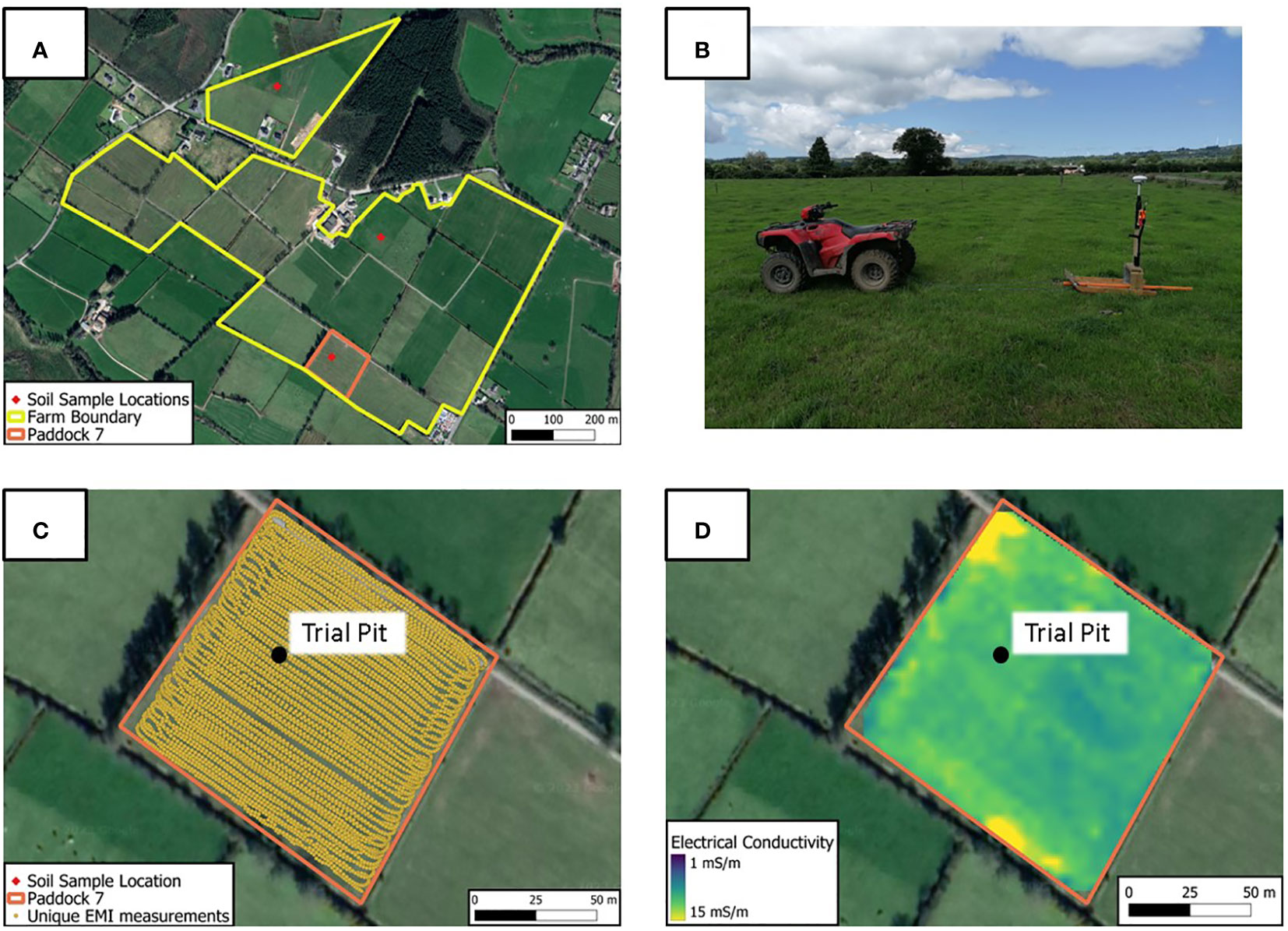
Figure 5 Site description - Ireland. (A) Outline of farm and study field and Trial Pit locations, (B) EMI set up, (C) EMI measurement locations in Paddock 7 with Trial pit location, (D) Measured electrical conductivity (0.5 m coil separation), processed, and gridded to 1 x 1 m with Trial pit location.

A single instrument, a CMD Mini-Explorer 6L (39), was used to acquire EMI data. This was towed on a GPS equipped wooden sled behind a quad bike, at ~ 2 m distance (Figure 5B). An average speed of 5 – 7 km/h was maintained, with an inline spatial sampling frequency of 10 Hz, giving an inline separation of ~ 0.2 m and a crossline distance of ~ 1.5 - 2 m (Figure 5C). This instrument has 6 receiver coils with separations of 0.2, 0.33, 0.5, 0.72, 1.03, 1.5 m.

For this study a single paddock, P7, was selected to demonstrate the proposed methodology. It is 1.31 ha in area, has typical surface water gley soil (59) and there is one location where quantitative measurements of some soil physical properties were collected in October 2015 (Table 2). This field was selected as it demonstrates intra-field variation in EMI measurements where ground data are sparse.

Table 2

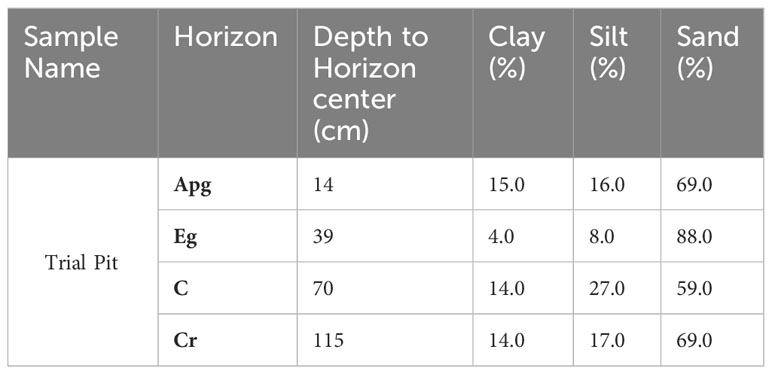
Table 2 Soil physical properties for Paddock 7.

P7 was acquired on 30^th August 2021. After data processing 5,625 EMI measurement locations (Figure 5C) were gridded to a 1 x 1 m regular grid. The EMI data selected with 0.2 m coil separation were discarded due to noise in these data from the presence of the sled. The data from the remaining separations were processed and gridded (Figure 5D) and used for clustering and inversion.

2.5 Linear regression between ECt and soil properties

To relate outputs from inversions to measured soil properties, this study uses linear regression (60) which is performed between inverted ECt and soil textural properties. ECt values are extracted from each Q3D inverted result at the closest (< 1 m) geographical EMI point and at the same sample depths as the soil textural properties measured in each site (Tables 1, 2). Therefore, there are as many analysis points as there are measured soil properties at all depths. This is used to indicate the relationship between a soil property and ECt values.

The metrics to show this relationship are coefficient of determination (R²) and root mean squared error (RMSE). A high R² value (~ 1) indicates that variance in ECt can explain variance in the soil property of interest and a low RMSE value (~ 0%) indicates good predictability. This analysis is performed at each sample location (Germany, Samples 5, 12, 13, 22 & 27; Ireland, Trial Pit) individually.

3 Results

3.1 Clustering results

An MCASD analysis of the EMI ECa data from the German site resulted in a maximum of 6 clusters to be appropriate (Figure 6A) with the option of 3, 4 or 6 clusters being appropriate for the Irish site Figure 6D). To provide the best compromise between MCASD stability metrics and initial model spatial resolution, the six-cluster solution is used in this study for both sites (more detail provided in Supplementary Figures 1, 2). For the German and Irish sites, the graphed MCASD metrics (Figures 6A, D) show that the 7-cluster and 5-cluster solutions, respectively are not stable over multiple clustering runs.

Figure 6

Figure 6 Clustering results for German (left) and Irish (right) sites: (A) MCASD analysis showing appropriate cluster numbers for field F22. (B) Spatial distribution of clusters in F22 with soil sample locations marked, (C) Cluster center data vectors for F22, D) MCASD analysis for field P7, (E) Spatial distribution of clusters in P7 with soil sample location marked, (F) Cluster center data vectors for P7, Ireland.

The spatial distribution of the 6-cluster solution for both Germany and Ireland (Figures 6B, E) is colored to match the corresponding cluster center (Figures 6C, D) and indicate areas of similar electrical conductivity. The German site shows a general decreasing ECa with increasing cluster number. The Irish site shows a greater change in ECa between cluster centers, with a relatively high electrical conductivity in the 0.33 and 0.5 m coil separation data layers in cluster 1, relating to the shallowest depths of investigation.

Soil sample locations on the German site are sometimes located geographically close to cluster center boundaries. Sample 5 is in a 1 m x 1m grid point assigned to cluster 3, but also < 1 m from a cluster 4 grid point. Sample 12 is in cluster 5 and ~ 4 m from any other clusters. Sample 13 is ~ 20 cm from a cluster boundary between cluster 4 and 5 and ~ 2 m from a cluster 3 grid point. Sample 22 is in cluster 5, and ~1.5 m from cluster 6. Sample 27 is in cluster 6. The single soil sample location on the Irish site is in cluster 4, and ~ 2.5 m from cluster 5.

3.2 Inversion results

3.2.1 Cluster center inversions

Cluster center data (Figures 6C, F) were input to EM4Soil 1D inversion algorithm with inversion parameters in section 2.2. The resulting 1D ECt profiles for the German site (Figure 7A) show electrical conductivity differences between the profiles at depths of ~ 0.5 m and between 1.5 m and 2.0 m. The Irish site (Figure 7B) differences are present to ~ 0.5 m depth. The cluster center colors match the spatial distribution of clusters (Figures 6B, E).

Figure 7

Figure 7 (A) Inverted cluster center profiles for Germany Field 22, (B) Inverted cluster center profiles for Ireland, Paddock 7.

The average RMSE between the cluster center (analogous to measured) ECa and the ECa obtained by forward modelling from the 1D ECt profiles is 0.23 mS/m for the German cluster center and 0.24 mS/m for the Irish cluster centers. This indicates a successful inversion was achieved.

3.2.2 Q3D inversions and comparison with physical property

Processed and gridded EMI data from both sites were input to EM4Soil Q3D inversion algorithm with all inversions performed using the parameters in section 2.2. For each site, an inversion was performed using a constant conductivity (10 mS/m) vs depth initial model. Subsequent inversions were then performed using ECt values of each of the cluster center models (Figure 7) as the initial model beneath each measurement location.

A linear regression between ECt values and soil texture at the same depths at each sample location is used to assess the accuracy of the model predictions (Table 3). In general, the use of a cluster center based initial model improves R² and RMSE. Samples 13 and 22 from the German site have only 3 measurements of soil properties and sample 13 has a decreased performance in R² and RMSE when using any cluster center initial model. The Irish site shows a significant improvement in both metrics when inversion is performed using a cluster center based initial model, but the dataset is very small.

Table 3

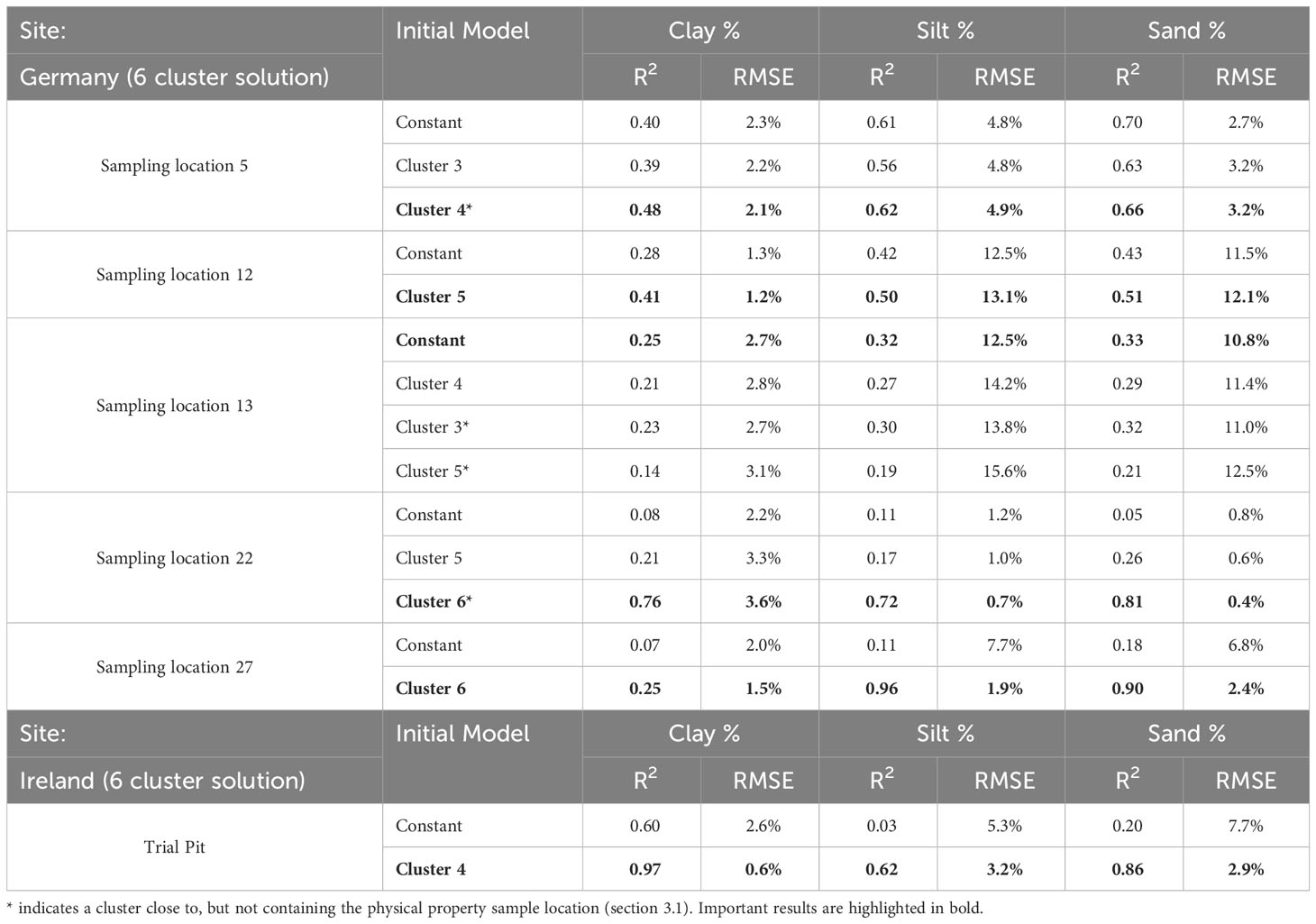
Table 3 Linear regression between ECt and soil texture data.

4 Discussion

4.1 Data processing

The use of EMI data for soil mapping is becoming more popular (19). This study performed a standardized processing flow to all data with no user input. Histogram (33) and Principal Component Analysis (40) filters provided much of the noise reduction. Both filters are data driven, and so adapt to the noise in the data. PCA requires a subjective choice of which components to retain in the filter and this study used the first two components which represented ~ 95% of the variability in the data. A standardized processing flow was applied as EMI instrument and acquisition parameters were very similar. While generally robust, this flow may not be appropriate for all EMI datasets due to different noise contributions for different surveys, which may require specific noise reduction strategies. PCA may only be applied to multi-coil/frequency instruments and so would not be appropriate for a single coil acquisition.

4.2 Self-organizing maps

EMI surveys are often used to “connect the dots” of traditional soil sampling campaigns. However, extensive soil sampling may not be practical at field scale. A key recommendation from this study is that EMI data should be used prior to traditional soil sampling to guide the locations of sampling, so reducing overall cost and maximizing understanding of soil property distribution across a site. This study demonstrates that clustering identifies areas where apparent conductivity data, and therefore soil property data, are likely to be similar. This would then allow for a cost-effective soil sampling campaign, where at least one sample per cluster could be taken after a cluster analysis of EMI survey data

One issue with clustering, regardless of the technique, is the choice of the number of clusters to represent a dataset. In this study, the MCASD stability metric (48) was used to determine an appropriate number of clusters for each dataset. The choice in this study to use the highest appropriate cluster number (coincidently six for both German and Irish sites), where the MCASD metric and range remain small, was to achieve the greatest spatial resolution in initial model variation across each site. MCASD also successful identified that the use of a 5-cluster solution, on the German data, was not appropriate (Supplementary Figure 2). It is also noted that using a lower cluster number did not significantly change the eventual link to soil properties (Supplementary Table 1), further justifying the use of the highest number of clusters as determined by MCASD analysis.

The combined use of unsupervised clustering (SOM) and MCASD allows for the objective grouping of EMI ECa data from both German and Irish sites (Figure 6), in contrast to the supervised classification used in Brogi et al. (22), which required additional local knowledge of expected soil types. Heil and Schmidhalter (28) conclude that interpretation of ECa measurements are highly location and soil specific and so the resulting spatial distributions from this SOM analysis could be used to guide a field sampling campaign, with minimal user input and background knowledge of expected soil property variation, aiding any conclusions drawn from an EMI survey.

4.3 Inversions and initial models

An inversion of EMI data provides a distribution of true subsurface electrical conductivity which, unlike ECa, can be related directly to soil physical properties. All inversion techniques are non-unique, especially in the presence of noise, in that there are trade-offs between the resolution of the retrieved model parameters (electrical conductivity distribution) and the fit between the model response and observed data. For the non-linear iterative inversion technique used in this study, there are choices related to constraining the limits and smoothness of the estimated 1D electrical conductivity distribution. These are subjective or can be linked to a priori soil physical properties which may, for example, demonstrate soil layering (32).

This study demonstrates how to remove some of the subjectivity related to non-linear iterative inversion of EMI data using cluster centers to help in the choice of the initial model which starts the inversion. The results (Table 3) confirm that the initial model is important when inverting ECa data and indicate applying the cluster center initial model for each measurement within the cluster can improve the correlations between electrical conductivity and soil texture. The approach provides a practical solution to potentially computationally time-consuming searches (e.g., Koganti et al. (60)) around the parameters of the inverted model to maximize these correlations.

In a similar method, reference point lateral constraint (61), the results of the inversion of a single data point are passed to the next data point as the initial model along a flight line in airborne EMI data. A current limitation of the method is that there is no software for the integration of a spatially variable initial model for Q3D inversions.

4.4 Implications for soil property monitoring

A requirement of advanced pedophysical (35) and agroecosystem models (31) is a knowledge of ECt distributions across a site. The methods presented produce such ECt distributions but their accuracy for predicting soil texture is unknown until soil samples are acquired. The choice of soil sample locations may improve the correlation between ECt and sub-surface static property variations using the clustering techniques presented in this paper. The results, (Table 3), particularly the German site which has strong heterogeneity (22), provide a prima facie demonstration of the efficacy of the technique. They also show that soil samples located close to cluster boundaries are less suitable for soil property prediction from ECt, likely due to clustering identifying areas of transition between soil physical properties. This implies that an EMI survey and clustering should be conducted prior to a soil sampling campaign to maximize efficiency.

ECt has a time-varying component as a consequence of the dynamic properties of the soil such as (a) saturation, which changes due to dynamic hydro-meteorological conditions, (b) electrical conductivity of the fluid with changing salinity and temperature in the interconnected pore space (62) and (c) changes in pore structure dynamics (i.e., bulk density, pore size distribution and connectivity) in agricultural regions (20, 63) due to tillage, compaction from animal/vehicle traffic and periods of bare soil (64). ECt also has a longer-term time-invariant component of the microgeometry of the pore space distribution (34, 65) associated with static soil properties, such as soil texture, the particle-size distribution (sand, silt, clay etc.), particle shape and orientation, and the type of clay minerals with their specific electrical properties which influence, e.g., cation exchange capacity. Disentangling the effect of each of these properties on ECt is difficult and often requires the use of physical property samples (21) or soil electrical conductivity models (65).

A separation of the relatively stable properties of texture from the dynamic state variables may be attempted by repeated EMI surveys over a wide range of hydro-meteorological and agricultural conditions. Multiple ECa datasets acquired at different times can be incorporated into the MCASD method, resulting in a single optimum number of stable clusters which should allow a comparison of ECt distributions temporally. Such analysis was demonstrated on optical satellite data (48). If additional ancillary data sets, such as volumetric soil moisture from time-domain reflectometry and fluid conductivity from conductivity-temperature-density sensors, are available, then a separation of the stable properties from dynamic state variables may be attempted also (66, 67).

In the context of additional multiple EMI and ancillary datasets, three open research questions are:

(a) whether the cluster centers of the ECa clusters provide ECt distributions at each acquisition time which are better correlated with the stable state variables of texture and clay-type at sample locations.

(b) whether the clustering-inversion approach can identify areas where ECt changes most rapidly with time.

(c) whether the temporal stability approach, applied to a single coil/frequency EMI instrument (66), can be improved by applying it to ECt derived from EMI instruments with multiple coil spacings using the clustering-inversion approach presented here.

5 Conclusions

This paper emphasizes the role of electromagnetic induction data for soil mapping. It focuses on its significance for developing a soil sampling strategy prior to soil sampling and its ability to link electrical conductivity to soil texture. A Self-Organizing Map (SOM), which is a neural network clustering technique, is used to classify electrical conductivity variations into distinct zones in two field sites. Clustering could help to ensure that subsequent soil sample data helps to calibrate succinctly the spatial variations of electrical conductivity in each field, so enhancing the precision of soil property prediction.

The clustering guides inversions of the EMI data by providing a practical solution to the choice of an initial model to start a 1D non-linear iterative inversion beneath each measurement in the context of a quasi-3D inversion of many data points at a site. The combination of EMI technology and progress in data processing and analytics promises to increase the capabilities of soil property characterization for more sustainable and environmentally responsible soil management strategies.

The methods can be applied to any EMI instrument, including those on large scale airborne surveys. Therefore, future work includes developing a software solution to incorporate a spatially varying initial model into Q3D inversions.

Data availability statement

The raw data supporting the conclusions of this article will be made available by the authors, without undue reservation.

Author contributions

DO’L: Conceptualization, Methodology, Writing – original draft. CosB: Resources, Writing – review & editing. ColB: Methodology, Validation, Writing – review & editing. PT: Writing – review & editing. ED: Methodology, Project administration, Supervision, Writing – review & editing.

Funding

The author(s) declare financial support was received for the research, authorship, and/or publication of this article. The initial German study was supported by the Deutsche Forschungsgemeinschaft through the Transregional Collaborative Research Center 32 – Patterns in Soil-Vegetation-Atmosphere Systems: Monitoring, Modelling and Data Assimilation. In addition, support was received through the “TERrestrial ENvironmental Observatories” (TERENO), and Advanced Remote Sensing—Ground-Truth Demo and Test Facilities (ACROSS) initiative and by the DFG (German Research Foundation) through the project 357874777, which is part of the research unit FOR 2694 Cosmic Sense. The Irish study was supported through Irish Research Council (IRC) PhD Scholarship award (GOIPG-2018-233). The CMD Mini-Explorer was purchased with an Equipment grant co-funded by the University of Galway and Teagasc.

Acknowledgments

The authors wish to thank the respective landowners for allowing access to their land. For the German site, we thank Marius Schmidt for his help in contacting the landowners, and Igor dal Bo, Philipp Pohlig, Luka Kurnjek, Liza de Quadros and Prakash Satenahalli for their help during the measurement campaign. For the Irish site, we thank Asaf Shnel and Eadaoin O’Raw for their help during the measurement campaign.

Conflict of interest

The authors declare that the research was conducted in the absence of any commercial or financial relationships that could be construed as a potential conflict of interest.

Publisher’s note

All claims expressed in this article are solely those of the authors and do not necessarily represent those of their affiliated organizations, or those of the publisher, the editors and the reviewers. Any product that may be evaluated in this article, or claim that may be made by its manufacturer, is not guaranteed or endorsed by the publisher.

Supplementary material

The Supplementary Material for this article can be found online at: https://www.frontiersin.org/articles/10.3389/fsoil.2024.1346028/full#supplementary-material

References

1. JRC. The State of Soil in Europe, European Soil Data Centre (ESDAC) (2012). Available at: https://esdac.jrc.ec.europa.eu/ESDB_Archive/eusoils_docs/other/EUR25186.pdf (Accessed 01/10/2023).

Google Scholar

2. EU. EU Soil Strategy for 2030 (2021). Available at: https://eur-lex.europa.eu/legal-content/EN/TXT/?uri=CELEX%3A52021DC0699 (Accessed 27/07/2023).

Google Scholar

3. UN. (2022). Available at: https://www.fao.org/fao-stories/article/en/c/1599222/ (Accessed 27/07/2023). Food and Agriculture Organization.

Google Scholar

4. Bünemann EK, Bongiorno G, Bai Z, Creamer RE, De Deyn G, de Goede R, et al. Soil quality – A critical review. Soil Biol Biochem (2018) 120:105–25. doi: 10.1016/j.soilbio.2018.01.030

CrossRef Full Text | Google Scholar

5. UN. Do you know all 17 SDGs? (2021). Available at: https://sdgs.un.org/goals (Accessed 24/10/2022).

Google Scholar

6. Bronick CJ, Lal R. Soil structure and management: A review. Geoderma (2005) 124(1-2):3–22. doi: 10.1016/j.geoderma.2004.03.005

CrossRef Full Text | Google Scholar

7. Faber JH, Cousin I, K.H.E. Meurer CMJ, Bispo A, Viketoft M, ten Damme L, et al. Stocktaking for Agricultural Soil Quality and Ecosystem Services Indicators and their Reference Values., EJP SOIL and EC Portal (2022). Available at: https://ejpsoil.eu/fileadmin/projects/ejpsoil/1st_call_projects/SIREN/SIREN_D2_final_report.pdf (Accessed 28/07/2023).

Google Scholar

8. McBratney AB, Santos MLM, Minasny B. On digital soil mapping. Geoderma (2003) 117(1-2):3–52. doi: 10.1016/S0016-7061(03)00223-4

CrossRef Full Text | Google Scholar

9. Zhang GL, Liu F, Song XD. Recent progress and future prospect of digital soil mapping: A review. J Integr Agr (2017) 16(12):2871–85. doi: 10.1016/S2095-3119(17)61762-3

CrossRef Full Text | Google Scholar

10. Román Dobarco M, McBratney A, Minasny B, Malone B. A framework to assess changes in soil condition and capability over large areas. Soil Secur (2021) 4:100011. doi: 10.1016/j.soisec.2021.100011

CrossRef Full Text | Google Scholar

11. Kibblewhite MG, Ritz K, Swift MJ. Soil health in agricultural systems. Philos T R Soc B (2008) 363(1492):685–701. doi: 10.1098/rstb.2007.2178

Google Scholar

12. Searchinger T, James O, Dumas P. Europe's Land Future? Opportunities to use Europes land to fight climate change and improve biodiversity;and why proposed policies could undermine both (2022). Available at: https://scholar.princeton.edu/tsearchi/publications/europes-land-future (Accessed 09/05/2022).

Google Scholar

13. Monteiro A, Santos S, Gonçalves P. Precision agriculture for crop and livestock farming-brief review. Animals (2021) 11:2345. doi: 10.3390/ani11082345

CrossRef Full Text | Google Scholar

14. Malone B, Stockmann U, Glover M, McLachlan G, Engelhardt S, Tuomi S. Digital soil survey and mapping underpinning inherent and dynamic soil attribute condition assessments. Soil Secur (2022) 6:100048. doi: 10.1016/j.soisec.2022.100048

CrossRef Full Text | Google Scholar

15. Cheng D, Yao Y, Liu R, Li X, Guan B, Yu F. Precision agriculture management based on a surrogate model assisted multiobjective algorithmic framework. Sci Rep (2023) 13(1):1142. doi: 10.1038/s41598-023-27990-w

PubMed Abstract | CrossRef Full Text | Google Scholar

16. Brogi C, Huisman JA, Weihermüller L, Herbst M, Vereecken H. Added value of geophysics-based soil mapping in agro-ecosystem simulations. Soil (2021) 7(1):125–43. doi: 10.5194/soil-7-125-2021

CrossRef Full Text | Google Scholar

17. Webster R. Digital Soil Mapping: An Introductory Perspective - Edited by Lagacherie P., McBratney A. B., Voltz M. Eur J Soil Sci (2007) 58:1217–8. doi: 10.1111/j.1365-2389.2007.00943_6.x

CrossRef Full Text | Google Scholar

18. Binley A, Hubbard S, Huisman J, Revil A, Robinson D, Singha K, et al. The emergence of hydrogeophysics for improved understanding of subsurface processes over multiple scales. Water Resour Res (2015) 51(6):3837–66. doi: 10.1002/2015WR017016

PubMed Abstract | CrossRef Full Text | Google Scholar

19. Boaga J. The use of FDEM in hydrogeophysics: A review. J Appl Geophysics (2017) 139:36–46. doi: 10.1016/j.jappgeo.2017.02.011

CrossRef Full Text | Google Scholar

20. Romero-Ruiz A, Linde N, Keller T, Or D. A review of geophysical methods for soil structure characterization. Rev Geophys (2018) 56(4):672–97. doi: 10.1029/2018RG000611

CrossRef Full Text | Google Scholar

21. Becker SM, Franz TE, Abimbola O, Steele DD, Flores JP, Jia X, et al. Feasibility assessment on use of proximal geophysical sensors to support precision management. Vadose Zone J (2022) 21:e20228. doi: 10.1002/vzj2.20228

CrossRef Full Text | Google Scholar

22. Brogi C, Huisman JA, Patzold S, von Hebel C, Weihermuller L, Kaufmann MS, et al. Large-scale soil mapping using multi-configuration EMI and supervised image classification. Geoderma (2019) 335:133–48. doi: 10.1016/j.geoderma.2018.08.001

CrossRef Full Text | Google Scholar

23. Zhao D, Li N, Zare E, Wang J, Triantafilis J. Mapping cation exchange capacity using a quasi-3d joint inversion of EM38 and EM31 data. Soil Tillage Res (2020) 200:104618. doi: 10.1016/j.still.2020.104618

CrossRef Full Text | Google Scholar

24. Fung E, Wang J, Zhao X, Farzamian M, Allred B, Clevenger WB, et al. Mapping cation exchange capacity and exchangeable potassium using proximal soil sensing data at the multiple-field scale. Soil Tillage Res (2023) 232:105735. doi: 10.1016/j.still.2023.105735

CrossRef Full Text | Google Scholar

25. Huth NI, Poulton PL. An electromagnetic induction method for monitoring variation in soil moisture in agroforestry systems. Aust J Soil Res (2007) 45(1):63–72. doi: 10.1071/SR06093

CrossRef Full Text | Google Scholar

26. Koganti T, Narjary B, Zare E, Pathan AL, Huang J, Triantafilis J. Quantitative mapping of soil salinity using the DUALEM-21S instrument and EM inversion software. Land Degrad Dev (2018) 29(6):1768–81. doi: 10.1002/ldr.2973

CrossRef Full Text | Google Scholar

27. Farzamian M, Bouksila F, Paz AM, Santos FM, Zemni N, Slama F, et al. Landscape-scale mapping of soil salinity with multi-height electromagnetic induction and quasi-3d inversion in Saharan Oasis, Tunisia. Agric Water Manage (2023) 284:108330. doi: 10.1016/j.agwat.2023.108330

CrossRef Full Text | Google Scholar

28. Heil K, Schmidhalter U. The application of EM38: Determination of soil parameters, selection of soil sampling points and use in agriculture and archaeology. Sensors (2017) 17(11):2540. doi: 10.3390/s17112540

PubMed Abstract | CrossRef Full Text | Google Scholar

29. Romero-Ruiz A, O'Leary D, Daly E, Tuohy P, Milne A, Coleman K, et al. Detection of spatial variability in soil compaction due to grazing using field-scale electromagnetic induction data and agro-geophysical modelling. Soil Use Manage Accepted (2023).

Google Scholar

30. Doolittle JA, Brevik EC. The use of electromagnetic induction techniques in soils studies. Geoderma (2014) 223:33–45. doi: 10.1016/j.geoderma.2014.01.027

CrossRef Full Text | Google Scholar

31. Garré S, Blanchy G, Caterina D, De Smedt P, Romero-Ruiz A, Simon N. Geophysical methods for soil applications, Reference Module in Earth Systems and Environmental Sciences. Elsevier (2022). doi: 10.1016/B978-0-12-822974-3.00152-X

CrossRef Full Text | Google Scholar

32. Triantafilis J, Monteiro Santos FA. Electromagnetic conductivity imaging (EMCI) of soil using a DUALEM-421 and inversion modelling software (EM4Soil). Geoderma (2013) 211-212:28–38. doi: 10.1016/j.geoderma.2013.06.001

CrossRef Full Text | Google Scholar

33. von Hebel C, Rudolph S, Mester A, Huisman JA, Kumbhar P, Vereecken H, et al. Three-dimensional imaging of subsurface structural patterns using quantitative large-scale multiconfiguration electromagnetic induction data. Water Resour Res (2014) 50(3):2732–48. doi: 10.1002/2013WR014864

CrossRef Full Text | Google Scholar

34. Revil A, Cathles Iii LM, Losh S, Nunn JA. Electrical conductivity in shaly sands with geophysical applications. J Geophysical Research: Solid Earth (1998) 103(B10):23925–36. doi: 10.1029/98JB02125

CrossRef Full Text | Google Scholar

35. Veirana GM, Smedt PD, Cornelis W, Hanssens D, Verhegge J. A theoretical approach to near surface pedophysical permittivity models. (2021) NSG2021 27th European Meeting of Environmental and Engineering Geophysics 2021(1):1–5. doi: 10.3997/2214-4609.20212020

CrossRef Full Text | Google Scholar

36. Saey T, De Smedt P, Delefortrie S, Van De Vijver E, Van Meirvenne M. Comparing one- and two-dimensional EMI conductivity inverse modeling procedures for characterizing a two-layered soil. Geoderma (2015) 241-242:12–23. doi: 10.1016/j.geoderma.2014.10.020

CrossRef Full Text | Google Scholar

37. McNeill JD. Electromagnetic terrain conductivity measurement at low induction numbers (1980). Available at: https://cir.nii.ac.jp/crid/1572543024212993792.

Google Scholar

38. Everett ME, Chave AD. On the physical principles underlying electromagnetic induction. Geophysics (2019) 84(5):W21–32. doi: 10.1190/geo2018-0232.1

CrossRef Full Text | Google Scholar

39. GF Instruments. CMD Electromagnetic conductivity meter user manual V. 1.5 & 2.1. Available at: http://www.gfinstruments.cz/index.php?menu=gi&cont=cmd_ov (Accessed 01/08/2023).

Google Scholar

40. Minsley BJ, Smith BD, Hammack R, Sams JI, Veloski G. Calibration and filtering strategies for frequency domain electromagnetic data. J Appl Geophysics (2012) 80(C):56–66. doi: 10.1016/j.jappgeo.2012.01.008

CrossRef Full Text | Google Scholar

41. Christiansen AV, Pedersen JB, Auken E, Søe NE, Holst MK, Kristiansen SM. Improved geoarchaeological mapping with electromagnetic induction instruments from dedicated processing and inversion. Remote Sens (2016) 8:1022. doi: 10.3390/rs8121022

CrossRef Full Text | Google Scholar

42. Auken E, Christiansen AV. Layered and laterally constrained 2D inversion of resistivity data. Geophysics (2004) 69(3):752–61. doi: 10.1190/1.1759461

CrossRef Full Text | Google Scholar

43. Monteiro Santos FA, Triantafilis J, Bruzgulis K. A spatially constrained 1D inversion algorithm for quasi-3D conductivity imaging: Application to DUALEM-421 data collected in a riverine plain. Geophysics (2011) 76(2):B43–53. doi: 10.1190/1.3537834

CrossRef Full Text | Google Scholar

44. EMTOMO. EM4Soil: Software for Electromagnetic Tomography (2013). Available at: http://www.emtomo.com/home/ (Accessed 28/07/2023).

Google Scholar

45. Sasaki Y. Two-dimensional joint inversion of magnetotelluric and dipole-dipole resistivity data. Geophysics (1989) 54(2):254–62. doi: 10.1190/1.1442649

CrossRef Full Text | Google Scholar

46. Kaufman L. Finding groups in data an introduction to cluster analysis. Hoboken, N.J: Wiley-Interscience (2005). doi: 10.1002/9780470316801

CrossRef Full Text | Google Scholar

47. Wang Y, Ksienzyk AK, Liu M, Brönner M. Multigeophysical data integration using cluster analysis: assisting geological mapping in Trøndelag, Mid-Norway. Geophys J Int (2021) 225(2):1142–57. doi: 10.1093/gji/ggaa571

CrossRef Full Text | Google Scholar

48. O'Leary D, Brown C, Healy MG, Regan S, Daly E. Observations of intra-peatland variability using multiple spatially coincident remotely sensed data sources and machine learning. Geoderma (2023) 430:116348. doi: 10.1016/j.geoderma.2023.116348

CrossRef Full Text | Google Scholar

49. Kohonen T. Essentials of the self-organizing map. Neural Networks (2013) 37:52–65. doi: 10.1016/j.neunet.2012.09.018

PubMed Abstract | CrossRef Full Text | Google Scholar

50. Celebi ME, Kingravi HA, Vela PA. A comparative study of efficient initialization methods for the k-means clustering algorithm. Expert Syst With Appl (2013) 40(1):200–10. doi: 10.1016/j.eswa.2012.07.021

CrossRef Full Text | Google Scholar

51. Valentine A, Kalnins L. An introduction to learning algorithms and potential applications in geomorphometry and Earth surface dynamics. Earth Surf Dynam (2016) 4(2):445–60. doi: 10.5194/esurf-4-445-2016

CrossRef Full Text | Google Scholar

52. Delgado S, Higuera C, Calle-Espinosa J, Morán F, Montero F. A SOM prototype-based cluster analysis methodology. Expert Syst With Appl (2017) 88:14–28. doi: 10.1016/j.eswa.2017.06.022

CrossRef Full Text | Google Scholar

53. Benabdellah AC, Benghabrit A, Bouhaddou I. A survey of clustering algorithms for an industrial context. Proc Comput Sci (2019) 148:291–302. doi: 10.1016/j.procs.2019.01.022

CrossRef Full Text | Google Scholar

54. IUSS Working Group. World Reference Base For Soil Resources 2014, Update 2015 International Soil Classification System For Naming Soils And Creating Legends For Soil Maps (2015). Available at: https://www.fao.org/3/i3794en/I3794en.pdf (Accessed 27/09/2023).

Google Scholar

55. Brogi C, Huisman JA, Herbst M, Weihermüller L, Klosterhalfen A, Montzka C, et al. Simulation of spatial variability in crop leaf area index and yield using agroecosystem modeling and geophysics-based quantitative soil information. Vadose Zone J (2020) 19(1):e20009. doi: 10.1002/vzj2.20009

CrossRef Full Text | Google Scholar

56. Teagasc. Heavy Soils Programme (2017). Available at: https://www.teagasc.ie/crops/grassland/heavy-soils/ (Accessed 01/09/2023).

Google Scholar

57. Creamer R, O'Sullivan L. The Soils of Ireland. Springer International Publishing (2018). doi: 10.1007/978-3-319-71189-8

CrossRef Full Text | Google Scholar

58. Teagasc. Moorepark Dairy Levy Research Update. Teagasc heavy soils programme – lessons learned (2021). Available at: https://www.teagasc.ie/media/website/publications/2021/Heavy-Soils-Lessons-Learned_May-2021.pdf (Accessed 03/11/23).

Google Scholar

59. Creamer R. Irish SIS final technical report 13: Irish Soil Information System Legend. The Environmental Protection Agency Ireland: Secure Archive for environmental research data (2014). Available at: http://erc.epa.ie/safer/resource?id=38a6e9e9-4364-11e4-b233-005056ae0019.

Google Scholar

60. Koganti T, Moral FJ, Rebollo FJ, Huang J, Triantafilis J. Mapping cation exchange capacity using a Veris-3100 instrument and invVERIS modelling software. Sci Total Environ (2017) 599-600:2156–65. doi: 10.1016/j.scitotenv.2017.05.074

PubMed Abstract | CrossRef Full Text | Google Scholar

61. Zhang J, Huang C, Feng B, Shi Y. Inversion of airborne transient electromagnetic data based on reference point lateral constraint. J Appl Geophysics (2022) 202:104675. doi: 10.1016/j.jappgeo.2022.104675

CrossRef Full Text | Google Scholar

62. Corwin DL, Lesch SM. Apparent soil electrical conductivity measurements in agriculture. Comput Electron Agr (2005) 46(1):11–43. doi: 10.1016/j.compag.2004.10.005

CrossRef Full Text | Google Scholar

63. Schwen A, Zimmermann M, Bodner G. Vertical variations of soil hydraulic properties within two soil profiles and its relevance for soil water simulations. J Hydrol (2014) 516:169–81. doi: 10.1016/j.jhydrol.2014.01.042

CrossRef Full Text | Google Scholar

64. Meurer K, Barron J, Chenu C, Coucheney E, Fielding M, Hallett P, et al. A framework for modelling soil structure dynamics induced by biological activity. Global Change Biol (2020) 26(10):5382–403. doi: 10.1111/gcb.15289

CrossRef Full Text | Google Scholar

65. Wang H, Revil A. Surface conduction model for fractal porous media. Geophysical Res Lett (2020) 47(10):e2020GL087553. doi: 10.1029/2020GL087553

CrossRef Full Text | Google Scholar

66. Abdu H, Robinson D, Boettinger J, Jones SB. Electromagnetic induction mapping at varied soil moisture reveals field-scale soil textural patterns and gravel lenses. Front Agric Sci Eng (2017) 4(2):135–45. doi: 10.15302/J-FASE-2017143

CrossRef Full Text | Google Scholar

67. Martini E, Werban U, Zacharias S, Pohle M, Dietrich P, Wollschläger U. Repeated electromagnetic induction measurements for mapping soil moisture at the field scale: validation with data from a wireless soil moisture monitoring network. Hydrol Earth Syst Sci (2017) 21(1):495–513. doi: 10.5194/hess-21-495-2017

CrossRef Full Text | Google Scholar