Analyses of the Photospheric Magnetic Dynamics in Solar Active Region 11117 Using an Advanced CESE-MHD Model

Introduction

It is well known that the magnetic evolution of solar active regions (ARs) holds the key to understanding solar eruptive events such as flares, filament eruptions, and coronal mass ejections. Particularly, the evolution of the three-dimensional (3D) magnetic configuration should be able to give us the crucial information for the initiation of solar eruptive events as suggested by Schrijver (2011). In recent years, many magnetic parameters have been used with the intention to predict the initiation of solar eruptive events, such as the surface magnetic free energy (Leka and Barnes, 2003; Falconer et al., 2006; Wu et al., 2009), the unsigned magnetic fluxes and electric currents (Falconer, 2001; Falconer et al., 2003; Schrijver, 2007; Georgoulis and Rust, 2007), as well as magnetic shear (Falconer, 2001; Falconer et al., 2003). However, all these parameters are directly derived from the magnetic field measurements confined on the solar surface (i.e., the photosphere). To measure the 3D coronal magnetic field is still beyond our reach, thus it leads us to seek numerical modeling (simulation) to fulfill the void region of measurements, namely to deduce the magnetic field topology and strength in the higher layers of solar atmosphere from the measured photospheric magnetic field.

Recently, there are studies using nonlinear force-free field (NLFFF) extrapolations to investigate the structures and evolution of the coronal magnetic field in solar active regions. For example, Tadesse et al. (2012) have used a NLFFF code to investigate NOAA AR 11117 (which is also the target AR of the present study) to determine the sources of flare activity and temporal evolution between pre- and post-flare stages using measured vector magnetic fields from Synoptic Optical Long-term Investigation on the Sun (SOLIS). We have also demonstrated that analyses based on NLFFF modeling can shed important lights for the understanding the physics of the solar eruptive events (Jiang et al., 2014). However, in the NLFFF modeling, the effect due to interaction of magnetic field with plasma is totally omitted, which seems to be not realistic because the coronal plasma β (ratio of plasma thermal pressure to magnetic pressure) is actually larger than what can be negligible (Peter et al., 2015). Also the photospheric magnetic field is far from force-free, which conflicts with the assumption of force-freeness. Consequently, the NLFFF model regards the bottom of extrapolation as the base of corona rather than the photosphere, and some kind of pre-processing of the original magnetogram is required to mitigate the problem. The limitations of the NLFFF model are also pointed by Wang and Liu (2015), who have given a comprehensive review concerning the evolution of the active region magnetic field associated with solar eruptions. They pointed out that a magnetohydrodynamic (MHD) model driven by data can provide a step forward in understanding the evolution of magnetic fields associated with flares.

We are already on the way of developing such a data-driven MHD model aimed for studying the dynamics of solar ARs (Wu et al., 2006; Jiang et al., 2012, 2013). In our previous CESE-MHD model (Jiang et al., 2012), we have used the SDO/HMI vector magnetogram as the bottom boundary conditions to calculate a time-sequence of 3D MHD equilibria for mimic the AR evolution. But that model is designed for simulating only the corona, since the bottom boundary of the model is also assumed to be the coronal base, similarly as in the NLFFF models. Here we report our first attempt of characterizing a more realistic solar atmosphere by including in the model a plasma with temperature stratified from the photosphere to the corona. In this way, the solution can be used to simulate the MHD equilibrium for solar atmosphere of the full domain from the thin layers of photosphere, chromosphere and transition region until to the corona. We then apply our new model to AR 11117 in a time interval around a C-class confined flare, and in particular, here we limit our study at the photosphere surface while an analysis of the coronal field dynamics will be left for another paper. We calculated the relevant parameters such as plasma flow, magnetic energy flux and helicity flux, which are important information of how the non-potentiality is transported from below the photosphere into the corona. The paper is structured as follows: we first describe the mathematical model and procedures of the simulation in Section The Data-Driven CESE-MHD Model, then the results of application to AR 11117 in Section Results, and we conclude in Sections Concluding Remarks.

The Data-Driven CESE-MHD Model

This model is developed similar to the data-driven active region evolution MHD model given by Wu et al. (2006) with a different numerical scheme. We solve a set of 3D, time-dependent, compressible MHD equations, and take into consideration of the highly-stratified atmosphere from the photosphere to the corona in a simplified way. In comparison to our previous action region evolution model (Wu et al., 2005, 2006), the effects of differential rotation and meridional flow together with the higher order transport (i.e., effective diffusion due to random motion of granules or supergranules, and cyclonic turbulence effects) are not included. It will improve the efficiency of the computation and as our focus is on the coronal field evolution which could lead to eruption, those higher order transport effects have limited importance on the magnetic field topology and its related properties for short term evolution study.

The initial setup of the model consists of constructing hydrostatic equilibrium of solar atmosphere and a potential field model based on the vertical component (B_z) of the vector magnetogram, and then we input the vector magnetogram (including the transverse field) at the bottom boundary to driven the evolution of the model, which can then be regarded as a way of modeling the realistic and dynamical corona. However, a real dynamical simulation by continuously inputting a time-series observed vector magnetograms (for example, Wu et al., 2009) has not been done here because of the limitations of the numerical procedure. Instead, we perform on each set of magnetogram via a relaxation process to a new MHD equilibrium solution which is then used to approximately represent a single snapshot of the solar atmosphere evolution, i.e., the physical conditions at a specific time. In the following we present more details of the model.

Model Equations

The set of governing equations are the conservation laws and magnetic induction equation as follows:

$\begin{array}{l}\frac{\partial \rho }{\partial t}+\nabla ·\left(\rho \text{v}\right)=0,\rho \frac{D\text{v}}{Dt}=-\nabla p+\text{J}\times \text{B}+\rho \text{g}+\nabla ·\left(\upsilon \text{v}\rho \nabla \text{v}\right),\end{array}$

$\begin{array}{ll}\frac{\partial \text{B}}{\partial t}=\nabla \times \left(\text{v}\times \text{B}\right),\frac{\partial T}{\partial t}+\nabla ·\left(T\text{v}\right)=\left(2-\gamma \right)T\nabla ·\text{v}+Q.& (1)\end{array}$

In these equations: ρ, v, B, T denote the plasma density, flow velocity, magnetic field and temperature, respectively; J is the electric current; p is the gas pressure given by p = ρRT with the gas constant R = 1.65 × 10⁴ m² s⁻²; γ is the specific heat ratio with value of 5/3; g is the solar gravity and is assumed to be constant as its photospheric value since we simulate from the photosphere to low corona with height less than 100 Mm. A small kinematic viscosity υ with a value of ~Δx²/Δt (Δx is the grid space and Δt is the time step in the numerical computation) is added for consideration of numerical stability. In this work we do not try to incorporate the complicated thermodynamic processes of the real corona, such as the thermal conduction and radiative losses [e.g., see numerical works by Abbett (2007), Fang et al. (2010)], which are difficult to be simulated directly and is not our focus. Instead, we simply use an ad-hoc heating function Q to preserve the highly-stratified temperature structure from the photosphere to the corona. Following the work of Abbett and Fisher (2003) and Leake and Arber (2006), this can be done by simply setting a Newton-cooling equation of the temperature

$\begin{array}{ll}Q=-\frac{T-T(t=0)}{\tau }& (2)\end{array}$

which can force the local temperature back to its pre-defined value (initial) T(t = 0) when it deviates from T(t = 0) on a time-scale τ. This is also reasonable since we are interested in only the nonlinear dynamic interactions between the plasma flow field and magnetic field. We use the typical values of photospheric parameters to normalize the equations, which are given in Table 1. Especially the length unit H₀ = RT₀/g_p is the pressure scale height at the photosphere.

TABLE 1

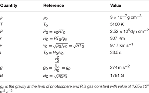
Table 1. Reference Values for Nondimensionalization.

The above equation system (1) is solved by our CESE-MHD code (Feng et al., 2007; Jiang et al., 2010). The CESE (Conservation Element and Solution Element) method deals with three-dimensional governing equations in a substantially different way that is unlike traditional numerical methods (e.g., the finite-difference or finite-volume schemes). The key principle, also a conceptual leap of the CESE method, is treating space and time as one entity. By introducing the CESEs as the vehicles for calculating the space-time flux, the CESE method can enforce conservation laws both locally and globally in their natural space-time unity form. Compared with many other numerical schemes, the CESE method can achieve higher accuracy with the same mesh resolution and provide simple mathematics and coding free of any type of Riemann solver or eigen-decomposition. For more detailed descriptions of the CESE method for MHD simulations including the multi-method control of the ∇ · B numerical errors, see our previous work, e.g., Feng et al. (2006, 2007) and (Jiang et al., 2010, 2011).

Initial Conditions

The initial configuration of the magnetic field simulation consists of a potential field matching the vertical component of the observed magnetogram and temperature-stratified plasma in hydrostatic equilibrium in the solar gravitational field. The potential field is obtained by a Green's function method (Metcalf et al., 2008). Because the magnetic field is measured on the photosphere surface, we also set the simulation volume extending from this very surface all the way to the corona, which can then describe self-consistently the behavior of the magnetic field in a highly stratified plasma with β from > 1 to < < 1 (Gary, 2001). This differs from the NLFFF model. To simulate a continuous temperature distribution from the photosphere (~ 5000 K) to the corona (~ 1 MK) in the solar atmosphere, we use a simple normalized stratified temperature model similar to those given by Wu et al. (2005),

$\begin{array}{ll}T\left(z\right)=1+\frac{T_{cor}-1}{2}\left[\text{tanh}\left(\frac{z-z_{tr}}{w_{tr}}\right)+1\right]& (3)\end{array}$

where z is the height from the photosphere, e.g., z = 0 represents the photosphere surface, the coronal temperature T_cor = 1 × 10⁶ K/T₀, and z_tr and w_tr represent the height and width of the transition region with z_tr = 3.75 Mm/H₀ and w_tr = 0.75 Mm/H₀. The density and gas pressure on the photosphere are assumed to be uniform. According to the hydrostatic equilibrium equation

$\begin{array}{ll}\frac{dp}{dz}=-\rho =-\frac{p}{T}& (4)\end{array}$

we have

$\begin{array}{l}p\text{}\left(z\right)=\exp \left[-{\displaystyle {\int }_0^z\frac{1}{T\left(z\prime \right)}dz\prime }\right]=[{\left(\frac{T\left(z\right)}{T\left(0\right)}\right)}^{1-1/T_{cor}}\\ {\left(\frac{T\left(0\right)-1}{T\left(z\right)-1}\right){\left(\frac{T_{cor}-T\left(z\right)}{T_{cor}-T\left(0\right)}\right)}^{1/T_{cor}}]}^{w_{tr}/2}.& (5)\end{array}$

Figure 1 shows the typical configuration of the parameters along a vertical line through the computation volume.

FIGURE 1

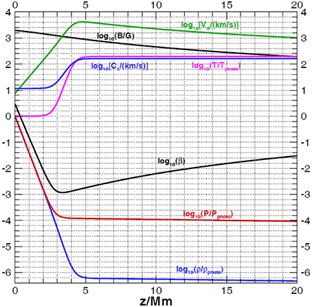
Figure 1. The typical configuration of the parameters along a vertical line through the computation volume including the density ρ, the gas pressure p, the temperature T, the magnetic field strength B, the Alfvén speed V_A, the gas sound speed C_s and the plasma β.

Computation Grid

In order to obtain optimal resolution of the computed physical properties, a special grid system is adopted. The horizontal grid is uniform with resolution as that of the magnetogram. In the vertical direction a non-uniform mesh is designed to both resolve the large gradient of the plasma parameters near the photosphere and meanwhile avoid too much computational overhead. We take advantage of our CESE-MHD code that can deal with general curvilinear grid by mapping a non-uniform physical grid onto a uniform reference grid. Here the mapping is defined as dx/dξ = dy/dη = H_m (normalized) and

$\begin{array}{ll}\frac{dz}{d\zeta }=\{\begin{array}{ll}k\hfill & \text{if}{\zeta }_1<{\zeta }_1\hfill \\ k+\frac{H_m-k}{2}\left[1-\cos \left(\frac{\pi \left(\zeta -{\zeta }_1\right)}{w\zeta }\right)\right]\hfill & \text{if}{\zeta }_1\le \zeta \le {\zeta }_1+w_{\zeta }\hfill \\ H_m\hfill & \text{if}{\zeta }_1<{\zeta }_1+w_{\zeta }\hfill \end{array}& (6)\end{array}$

with H_m is the pixel size of the magnetogram. For the present work we choose H_m = 2.4, k = 0.25, ζ₁ = 80, w_ζ = 80. In the reference space we use uniform grid d_ξ = d_η = d_ζ = 1. In this way the photosphere and the whole transition region z ∈ [0,5] Mm is resolved with a grid spacing of 0.25 times the scale height H₀ on the photosphere surface.

Besides the setup of spatial grid, we also need careful consideration for the time step. According to the CESE method, the numerical viscosity will become very large if the ratio of the actual time step to the local time step is small, especially when this ratio is smaller than 0.1 (Zhang et al., 2004). As shown in Figure 1, the Alfvén speed v_A increases from several km/s to 10³ km/s within the height of 5 Mm which is covered by a nearly uniform grid of Δz = 0.25H₀ ≈ 70 km. Thus the sharply increased Alfvén speed gives a sharply decreased local time step according to the Courant-Friedrichs-Lewy (CFL) stable condition Δt∝ Δz/v_A. If an uniform time step is used, the ratio to the local time step near the photosphere, e.g., z ≤ 1 Mm can be smaller than 0.01. This will result a very large numerical viscosity to the near-photosphere region, making the information difficult to pass through the high-β layer to the corona. Thus it is necessary to use a variable time step algorithm and here we use the time step directly according to the local time step. The detailed algorithm of using variable time step proportioned to the local grid spacing is described in Jiang et al. (2010) and here the only difference with the previous code is also to allow the time step variable according to the local wave speed.

Boundary Conditions

The computational domain includes six planes (i.e., four sided planes, top, and bottom). The boundary conditions used for the four sides and top plane are non-reflective. In order to accommodate the observation at the bottom boundary, the evolutionary boundary conditions must be used; thus, the method of projected characteristics, originated by Nakagawa (1981a,b) and implemented by Wu and Wang (1987) is used for the derivation of such boundary conditions. The briefly described derivation and its resulting time-dependent boundary conditions are given in the Appendix of Wu et al. (2006) and thus will not be repeated here.

Results

Here we apply the model to study AR 11117 around the time of a small flare. Since a rather full description of AR 11117 has been given in our previous paper (Jiang et al., 2012), we only briefly summarize some of the highlights here for completeness. During the Carrington Rotation (CR) 2101, the HMI on-board SDO has measured the 3 magnetic field components on the Sun's surface from October 20 – November 2, 2010. On the 25th of October 2010, this region became active with several small B-class flares being observed and near the end of the day, a C2.3-class flare occurred. GOES (Geostationary Operational Environmental Satellite) 15 recorded a soft x-ray event which began at 22:06UT, reaching a peak at 22:12UT and ending at 22:18UT as shown in the Figure 2. From observations recorded by AIA/SDO, it shows that only the central part of the active region is associated with the flare as shown in Figure 2. It indicates that the flare is confined to a low altitude without inducing significant changes to cause eruption of these coronal loops.

FIGURE 2

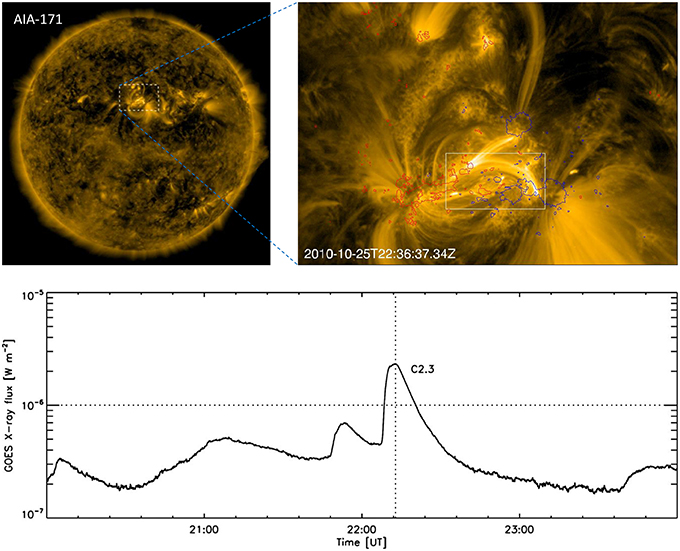
Figure 2. Top left: a full-disk SDO/AIA 171 $\stackrel{°}{A}$ image showing the location of AR 11117. Top right: AIA-171 image of the post-flare loops about 20 min after the flare peak time. The contour lines for the photospheric field B_r of −500 G (blue) and 500 G (red) are overlaid. Supplementary Video 1 shows the evolution of B_r from 21:00 to 23:00 UT of the same field of view. The boxed region denotes the field of view shown in Figure 4. Bottom: GOES soft-X ray flux from 20:00 UT to 24:00 UT on 2010 October 25 in the wavelength range of 1–8 $\stackrel{°}{A}$. The horizontal dotted line indicates the C-minor flare class and the vertical dotted line indicates the peak time of the flux.

We have chosen a sequence of vector magnetograms measured by HMI/SDO close to the C-class flare. Specifically the sequence of magnetograms was taken at 21:00, 21:36, 22:00, 22:12, 22:36, and 23:00 UT. By input of the measured vector magnetograms for a specific time at the lower boundary of the model, we obtain the MHD equilibrium solution for each of the input of vector magnetic field. Those solutions are used to approximately represent the snapshot of the solar atmosphere at that specific time.

Figure 3 shows the coronal magnetic field configuration and its comparison with the AIA-171 observations at 21:00 UT as an example. Overall the morphology of the simulated magnetic resembles the EUV observations. Especially, the traced coronal loops are matched well by the magnetic field lines. When examining the change of the magnetic field configuration in the different times, we find it is not easy to recognize. This is because the flare is a confined flare without eruption and the basic coronal-loop system as observed from AIA-171 shows very small changes, but reconnection at a magnetic topology surface might cause the flare, as suggested by Jiang et al. (2012).

FIGURE 3

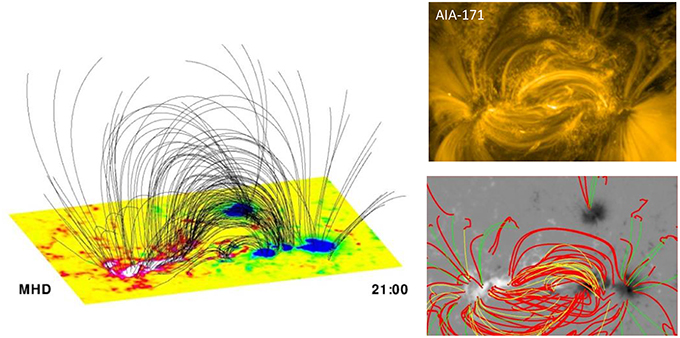
Figure 3. Left: 3D magnetic field lines from the MHD model for time of 21:00 UT. The bottom surfaces show the photospheric magnetic flux distribution (i.e., B_r), with white color as above 1000 G and blue as below −1000 G. Top right: AIA-171 image at the same time of 21:00 UT. Bottom right: comparison of coronal loop tracers and the magnetic field lines. The coronal loops are traced by a method of Gary et al. (2014) and are shown by the thin curves, and loops are colored yellow if they appear to be closed field lines, and green if they appear to be open field lines. The magnetic field lines are shown by the thick red curves and they are generated from the foot points of the coronal loops. The background is shown by the photospheric B_r.

The flaring loop system appears to be connected with the polarities at the southwest of the AR (see Figure 2). There, the apparent movement of the photospheric magnetic flux clearly show shearing and rotation, as can be seen in a movie of the HMI magnetogram (see the Supplementary Video 1). The small positive polarity (denoted by P in the movie) moves to the east (i.e., left of the field of view) with respect to its neighboring negative polarities. The negative polarity that has a circular shape (denoted by N in the movie) seems to rotate clockwise, and at the same time, moves to the west, squeezing the negative polarities in its west. Such features of photospheric motion is captured by our model to some extent. As can be seen in the top left panel of Figure 4, which shows the transverse velocity field obtained from the simulation at time 22:00 UT, shearing of the polarities is clear, and there is distinctly a clockwise vortex pattern of the velocity for the circular negative polarity (results for the other simulated times are similar and are not repeated here). Thus, both the observation and our simulation indicate a build-up of magnetic stress, which drives the coronal field further away from a potential-field state. The results based our previous model did not reproduce such a plasma flow at its bottom surface, likely because of its over-simplification of the plasma model.

FIGURE 4

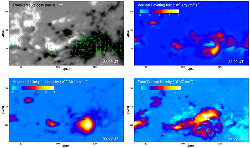
Figure 4. Top left: the transverse velocity of plasma with the background shown by the photospheric B_r. Top right: Poynting flux through the photosphere surface. Bottom left: magnetic helicity flux. Bottom right: total current helicity on the photosphere. The time is 22:00 UT, 2010 Oct 25. Field of view as shown are mentioned in Figure 2.

To further quantify the transport of magnetic non-potentiality across the photosphere, we calculated parameters including the Poynting flux, the magnetic helicity flux, and the current helicity at the surface, which are defined in the following, respectively:

Poynting flux, i.e., the amount of magnetic energy flux across the lower boundary (photosphere) to the corona can be expressed as (Démoulin and Berger, 2003);

$\begin{array}{ll}\left(\frac{dE}{dt}\right)=\frac{1}{4\pi }{\displaystyle {\int }_{photo}(B_t·v_t)B_{n}dS}+\frac{1}{4\pi }{\displaystyle {\int }_{photo}{B}_t^2·v_{n}dS}& (7)\end{array}$

where the B_t and v_t are the transverse magnetic field and velocity, respectively, and B_n and v_n are the normal components of magnetic field and velocity, respectively. On the right side of Equation (9), the first term represents the surface flow effect and the second term is due to direct flux emergence from below the photosphere.

Magnetic helicity flux, i.e., the injection rate of relative helicity across the photosphere, can be expressed similarly as (Démoulin and Berger, 2003)

$\begin{array}{l}\left(\frac{dH}{dt}\right)=-2{\displaystyle {\int }_{photo}\left(A_p·v_t\right)B_{n}dS}+2{\displaystyle {\int }_{photo}\left(A_p·B_t\right)}\\ ·v_{n}dS& (8)\end{array}$

where A_p is the vector potential of a potential field specified by the observed flux distribution B_n on the surface.

The current helicity is defined as (Bao and Zhang, 1998)

$\begin{array}{ll}{H}_c=\text{B}·(\nabla \times \text{B})=B_n·{(\nabla \times \text{B})}_n+{\text{B}}_t·{(\nabla \times \text{B})}_t& (9)\end{array}$

which show that the current helicity can also be separated into two parts, one related to the parallel component in the direction of the line of sight to the observer and the other to the vertical one. From photospheric vector magnetograms, only the first term can be inferred, while with the MHD solutions, we can calculate fully the two terms, so we refer to our results as the total current helicity.

Again in Figure 4, we show the distributions of these parameters on the surface, at 22:00 UT as an example, since the changes of these distributions within the modeled time interval is not significant. The distribution of the flux means that the flux density is calculated for each pixel on the surface. By examining these results, we recognize that there is net positive injection of energy in the studied area (a sum of the total flux density within the area, see also Figure 5), although mixed signs of flux density can be seen. The results are consistent with the flow pattern of strong shearing and rotation. Considering that the magnetic flux content does not changed significantly in the studied duration, such injection of energy should mostly go to the non-potential energy. Figure 5 shows the total magnetic energy flux as a function of time, and its two components separately [i.e., the two terms of Equation (9)]. It is clearly seen that the majority of energy flux results from the first term of Equation (9), which is caused by transverse flow effect (i.e., shearing and rotation). Our analysis is further supported by the results of the relative helicity injection flux, which is directly correlated with the twisting motion of the flux. The current helicity, as a more direct indicator of the non-potentiality, again speaks for the same conclusion.

FIGURE 5

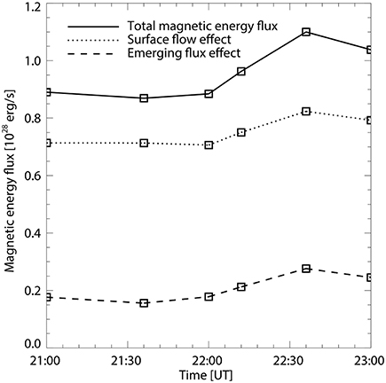
Figure 5. Computed different components of magnetic energy flux across the photosphere for AR 11117, 2010 Oct 25.

Concluding Remarks

In the present study, we present a modified CESE-MHD model constrained by the SDO/HMI vector magnetograms. By including a more realistic stratified atmosphere with a suitable grid design in both space and time, we are able to more closely mimic the MHD structures with behavior of β changing abruptly from > 1 (at the photosphere) to < < 1 (in the corona). For a specific AR around the time of a flare, we apply this model to study the photospheric surface dynamics which are thought to play an important role in the cause of energetic events in the solar corona. This advanced model calculates a coronal field matching the EUV coronal loops, and at the same time, recover the photospheric plasma flow field in reasonable agreement with the apparent motion of the magnetic polarities. By quantifying a set of physical properties such as the transverse velocity, Poynting flux, the relative helicity flux as well as the current helicity, we conclude that magnetic non-potentiality is injected into the corona in the simulated time interval, which might provide a favorable condition for producing the flare. The present work is a step forward in developing a realistic MHD model for simulating structure and evolution of solar AR's magnetic fields associated with solar eruptions. In a future work, we will pursuit a data-driven MHD analyses by input of a sequence of magnetic maps to study the true dynamics of the magnetic evolution leading to the flare.

Author Contributions

CJ and SW worked to put the paper together with the assistance of XF.

Conflict of Interest Statement

The authors declare that the research was conducted in the absence of any commercial or financial relationships that could be construed as a potential conflict of interest.

Acknowledgments

This work is supported by the 973 program under grant 2012CB825601, the Chinese Academy of Sciences (KZZD-EW-01-4), the National Natural Science Foundation of China (41574170, 41231068, 41274192, 41031066, and 41374176), and the Specialized Research Fund for State Key Laboratories, and Youth Innovation Promotion Association of CAS (2015122). CJ and SW are also supported by NSF-AGS1153323. Data are courtesy of NASA/SDO and the HMI science teams.

Supplementary Material

The Supplementary Material for this article can be found online at: https://www.frontiersin.org/article/10.3389/fspas.2016.00016

References

Abbett, W. P. (2007). The magnetic connection between the convection zone and corona in the quiet Sun. Astrophys. J. 665, 1469–1448. doi: 10.1086/519788

CrossRef Full Text | Google Scholar

Abbett, W. P., and Fisher, G. H. (2003). A coupled model for the emergence of active region magnetic flux into the solar corona. Astrophys. J. 582, 475–483. doi: 10.1086/344613

CrossRef Full Text | Google Scholar

Bao, S. D., and Zhang, H. Q. (1998). Patterns of current helicity for solar cycle 22. Astrophys. J. 496, L43–L46. doi: 10.1086/311232

CrossRef Full Text | Google Scholar

Démoulin, P., and Berger, M. A. (2003). Magnetic energy and helicity fluxes at the photospheric level. Solar Phys. 251, 203–215. doi: 10.1023/A:1025679813955

CrossRef Full Text

Falconer, D. A. (2001). A prospective method for predicting coronal mass ejections from vector magnetograms. J. Geophys. Res. Space Phys. 106, 25185–25190. doi: 10.1029/2000JA004005

CrossRef Full Text | Google Scholar

Falconer, D. A., Moore, R. L., and Gary, G. A. (2003). A measure from line−of−sight magnetograms for prediction of coronal mass ejections. J. Geophys Res. Space Phys. 108, 1380. doi: 10.1029/2003JA010030

CrossRef Full Text | Google Scholar

Falconer, D. A., Moore, R. L., and Gary, G. A. (2006). Magnetic causes of solar coronal mass ejections: dominance of the free magnetic energy over the magnetic twist alone. Astrophys. J. 644, 1258. doi: 10.1086/503699

CrossRef Full Text | Google Scholar

Fang, F., Manchester, W., Abbett, W. P., and van der Holst, B. (2010). Simulation of flux emergence from the convection zone to the corona. Astrophys. J. 714, 1649–1657. doi: 10.1088/0004-637X/714/2/1649

CrossRef Full Text | Google Scholar

Feng, X. S., Hu, Y. Q., and Wei, F. S. (2006). Modeling the resistive MHD by the CESE method. Solar Phys. 235, 235–257. doi: 10.1007/s11207-006-0040-6

CrossRef Full Text | Google Scholar

Feng, X. S., Zhou, Y. F., and Wu, S. T. (2007). A novel numerical implementation for solar wind modeling by the modified conservation element/solution element method. Astrophys. J. 655:1110. doi: 10.1086/510121

CrossRef Full Text | Google Scholar

Gary, G. A. (2001). Plasma beta above a solar active region: rethinking the paradigm. Solar Phys. 203, 71–86. doi: 10.1023/A:1012722021820

CrossRef Full Text | Google Scholar

Gary, G. A., Hu, Q., and Lee, J. K. (2014). A rapid, manual method to map coronal-loop structures of an active region using Cubic Bézier Curves and its applications to misalignment angle analysis. Solar Phys. 289, 847–865. doi: 10.1007/s11207-013-0359-8

CrossRef Full Text | Google Scholar

Georgoulis, M. K., and Rust, D. M. (2007). Quantitative forecasting of major solar flares. Astrophys. J. Lett. 661, L109. doi: 10.1086/518718

CrossRef Full Text | Google Scholar

Jiang, C. W., Feng, X. S., Fan, Y., and Xiang, C. (2011). Reconstruction of the coronal magnetic field using the CESE-MHD method. Astrophys. J. 727:101. doi: 10.1088/0004-637X/727/2/101

CrossRef Full Text | Google Scholar

Jiang, C. W., Feng, X. S., Wu, S. T., and Hu, Q. (2012). Study of the three-dimensional coronal magnetic field of active region 11117 around the time of a confined flare using a data-driven CESE-MHD model. Astrophys. J. 759:85. doi: 10.1088/0004-637X/759/2/85

CrossRef Full Text | Google Scholar

Jiang, C. W., Feng, X. S., Wu, S. T., and Hu, Q. (2013). Magnetohydrodynamic simulation of a sigmoid eruption of active region 11283. Astrophys. J. Lett. 771:L30. doi: 10.1088/2041-8205/771/2/L30

CrossRef Full Text | Google Scholar

Jiang, C. W., Feng, X. S., Zhang, J., and Zhong, D. K. (2010). AMR simulations of magnetohydrodynamic problems by the CESE method in curvilinear coordinates. Solar Phys. 267, 463–491. doi: 10.1007/s11207-010-9649-6

CrossRef Full Text | Google Scholar

Jiang, C. W., Wu, S. T., Feng, X. S., and Hu, Q. (2014). Formation and Eruption of an Active Region Sigmoid. I. A study by nonlinear force-free field modeling. Astrophys. J. 780:55. doi: 10.1088/0004-637X/780/1/55

CrossRef Full Text | Google Scholar

Leake, J. E., and Arber, T. D. (2006). The emergence of magnetic flux through a partially ionised solar atmosphere. Astron. Astrophys. 450, 805–818. doi: 10.1051/0004-6361:20054099

CrossRef Full Text | Google Scholar

Leka, K. D., and Barnes, G. (2003). Photospheric magnetic field properties of flaring versus flare-quiet active regions. I. Data, general approach, and sample results. Astrophys. J. 595:1277. doi: 10.1086/377511

CrossRef Full Text | Google Scholar

Metcalf, T. R., DeRosa, M. L., Schrijver, C. J., Barnes, G., van Ballegooijen, A. A., Wiegelmann, T., et al. (2008). Nonlinear force-free modeling of coronal magnetic fields. II. Modeling a filament arcade and simulated chromospheric and photospheric vector fields. Solar Phys. 247, 269–299. doi: 10.1007/s11207-007-9110-7

CrossRef Full Text | Google Scholar

Nakagawa, Y. (1981a). Evolution of magnetic field and atmospheric response. I-Three-dimensional formulation by the method of projected characteristics. II-Formulation of proper boundary equations. Astrophys. J. 247:707. doi: 10.1086/159082

CrossRef Full Text | Google Scholar

Nakagawa, Y. (1981b). Evolution of magnetic field and atmospheric responses-part two-formulation of proper boundary equations. Astrophys. J. 247:719. doi: 10.1086/159083

CrossRef Full Text | Google Scholar

Peter, H., Warnecke, J., Chitta, L. P., and Cameron, R. H. (2015). Limitations of force-free magnetic field extrapolations: revisiting basic assumptions. Astron. Astrophys. 584, A68. doi: 10.1051/0004-6361/201527057

CrossRef Full Text | Google Scholar

Schrijver, C. J. (2007). A characteristic magnetic field pattern associated with all major solar flares and its use in flare forecasting. Astrophys. J. Lett. 655:L117. doi: 10.1086/511857

CrossRef Full Text | Google Scholar

Schrijver, C. J. (2011). Long−range magnetic couplings between solar flares and coronal mass ejections observed by SDO and STEREO. J. Geophys. Res. Space Phys. 116, 2156–2202. doi: 10.1029/2010JA016224

CrossRef Full Text | Google Scholar

Tadesse, T., Wiegelmann, T., Inhester, B., and Pevtsov, A. (2012). Coronal magnetic field structure and evolution for flaring AR 11117 and its surroundings. Solar Phys. 281, 53–65. doi: 10.1007/s11207-012-9961-4

CrossRef Full Text | Google Scholar

Wang, H. M., and Liu, C. (2015). Structure and evolution of magnetic fields associated with solar eruptions. Res. Astron. Astrophys. 15, 145–174. doi: 10.1088/1674-4527/15/2/001

CrossRef Full Text | Google Scholar

Wu, S. T., Wang, A. H., and Falconer, D. A. (2005). IAU Symposium 226 on Coronal and Stellar Mass Ejections, eds K. P. Dere and J. X.Wang (Cambridge: Cambridge Univ. Press), 291.

Wu, S. T., Wang, A. H., Gary, G. A., Kucera, A., Rybak, J., Liu, Y., et al. (2009). Analyses of magnetic field structures for active region 10720 using a data-driven 3D MHD model. Advances Space Res. 44, 46–53. doi: 10.1016/j.asr.2009.03.020

CrossRef Full Text | Google Scholar

Wu, S. T., Wang, A. H., Liu, Y., and Hoeksema, J. T. (2006). Data-driven magnetohydrodynamic model for active region evolution. Astrophys. J. 652:800. doi: 10.1086/507864

CrossRef Full Text | Google Scholar

Wu, S. T., and Wang, J. F. (1987). Numerical tests of a modified full implicit continuous Eulerian (FICE) scheme with projected normal characteristic boundary conditions for MHD flows. Comput. Methods Appl. Mechanics Eng. 64, 267–282. doi: 10.1016/0045-7825(87)90043-0

CrossRef Full Text | Google Scholar

Zhang, M. J., Yu, S. T. J., and Chang, S. C. (2004). Solving magnetohydrodynamic equations without special treatment for divergence-free magnetic field. AIAA J. 42, 2605–2608. doi: 10.2514/1.8512

CrossRef Full Text | Google Scholar