Magneto-Rossby Waves and Seismology of Solar Interior

1. Introduction

Solar activity has tremendous influence on interplanetary space and the planets of the solar system including the Earth. It basically determines plasma conditions in the Earth's magnetosphere/ionosphere with possible harming effects on technological systems and human life. Therefore, solar activity prediction is very important scientific problem. Solar activity is characterized by 11 year quasi-periodic variation (Schwabe, 1844), but the underlying physical mechanism is not yet clear. The periodic increase/decrease of large-scale magnetic field is probably connected to some sort of magnetic dynamo which operates below or inside the convection zone owing to the existence of differential rotation and convection (Charbonneau, 2005). The magnetic field strength inside the dynamo layer is crucial to test different models, but the direct measurement is obviously complicated.

Besides the Schwabe cycle, solar activity also undergoes short term variations with the periods from several months to few years. The periodicity of 150–155 days was first discovered by Rieger et al. (1984) in strong solar flares. This periodicity has been later found in many indices of solar activity (Carbonell and Ballester, 1990; Oliver et al., 1998). Recently, Gurgenashvili et al. (2016) showed that the periodicity is anti-correlated with solar activity being shorter in stronger cycles, which probably means that the period depends on magnetic field strength in the internal dynamo layer. Then one can indirectly estimate the field strength if the generation mechanism of the periodicity is known. Several different mechanisms have been supposed from time to time to explain the periodicity, but more plausible reason seems to be connected with Rossby waves.

Rossby waves govern large scale dynamics of rotating sphere and are well studied in the Earth's atmosphere and oceans (Rossby, 1939; Gill, 1982). Recent direct observations of Rossby waves in coronal bright points based on STEREO and SDO observations (McIntosh et al., 2017) significantly increased the interest toward Rossby waves in the solar context. Lou (2000) suggested that the equatorially trapped hydrodynamic Rossby waves in the solar photosphere could explain Rieger-type periodicity in solar activity. Zaqarashvili et al. (2010a) showed that the instability of spherical Rossby waves in the solar tachocline owing to the joint action of the differential rotation and the toroidal magnetic field could give the observed periodicity. Recently Dikpati et al. (2017) showed that the nonlinear energy exchange between tachocline differential rotation and Rossby waves may occur over the time scales of Rieger-type periodicity, which might lead to the observed oscillations. Therefore, it is increasingly clear that a mechanism for the Rieger-type periodicity is related with Rossby waves in the tachocline.

Gurgenashvili et al. (2016) used the observed Rieger-type periodicities in sunspot numbers and dispersion relation of spherical 2D magnetic Rossby waves to estimate the magnetic field strength in the dynamo layer during solar cycles 14–24. Their estimations suggested a field strength of 40 kG in the stronger cycles 16–23 and 20 kG for the weaker cycles 14-15 and 24. The estimated field strength is favor for the dynamo models with tachocline rather than those without tachocline. However, using the simple dispersion relation of Rossby waves might lead to the rather rough estimation of the field strength and hence the conclusions could be overestimated. On the other hand, sub-adiabatic temperature gradient in the upper overshoot part of the tachocline creates negative buoyancy force resulting significant reduction of the gravity (Gilman, 2000; Dikpati and Gilman, 2001). The reduced gravity might lead to the concentration of shallow water waves around the equator. These equatorially trapped or equatorial waves (Matsuno, 1966) have quiet different periods comparing to those with the whole latitudinal extent. Using equatorial waves as the reasons for Rieger-type periodicity may change estimated strength of dynamo magnetic field.

Here we discuss the current achievements and future perspectives of Rossby-type waves in the estimation of dynamo magnetic field.

2. Rieger-Type Periodicity in Solar Activity

In this section, we present the evolution of Rieger-type periodicities over many solar cycles using the Greenwich Royal Observatory (GRO) daily and monthly sunspot area data, which are available from 1874 till 2016 (http://solarscience.msfc.nasa.gov/greenwch.shtml). GRO contains the records of the full disc data as well as sunspot area measurements for northern and southern hemispheres separately. Solar activity is not entirely homogeneous in the both hemispheres and sometimes has significantly different occurrence. The N-S asymmetry is seen in different indicators, such as sunspot area, sunspot number, group sunspot numbers, coronal mass ejections, solar flares, filaments, differential rotation, photospheric magnetic flux, post eruption arcades, polar field reversals, coronal green line intensity etc. This phenomenon was also presented during the Maunder minimum. Several authors reported strong hemispheric asymmetry in historical data which is claimed to be south-dominated. The GRO sunspot data correspond to the cycles 12–24, but the cycle 12 is not as reliable as other cycles, therefore we decided to use only the cycles 13–24.

Figures 1, 2 (upper panels) show the evolution of sunspot areas over the cycles 13–24 in the northern and the southern hemispheres respectively. It is clearly seen that the northern hemisphere was more active during the cycles 14–20, and the asymmetry was shifted to the southern hemisphere starting from the cycle 21. The north-south asymmetry is questionable in the cycle 13, but in the literature it is usually referred as south-dominated. It is possible that the transition from south to north domination occurred in this cycle. The corresponding lower panels of Figures 1, 2 display the Morlet wavelet analysis (Torrence and Compo, 1998) of the data, which shows the periodicity of amplitude variations. The wavelet analysis was also performed for each cycle separately to find the corresponding periodicity. Vertical solid lines correspond to solar activity minimum, while white lines encircle the most important powers above confidence level 99.9%. The Rieger periods that resulted from the global wavelet spectra are given in Table 1.

FIGURE 1

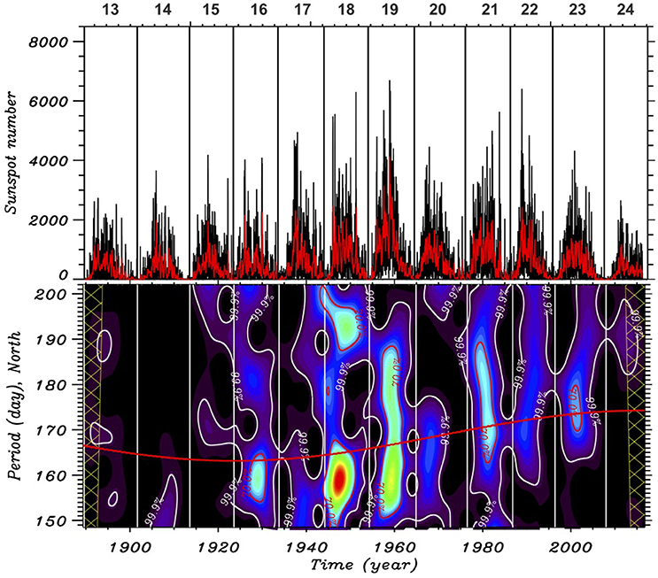
Figure 1. The upper panel represents GRO daily (black) and monthly averaged (red) hemispheric sunspot area data for cycles 13–24 for the northern hemisphere. The lower panel shows the corresponding wavelet analysis.

FIGURE 2

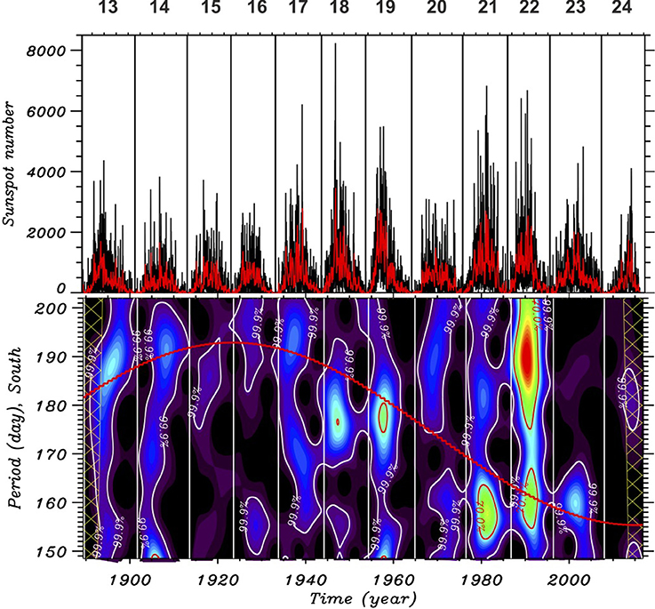
Figure 2. The upper panel represents GRO daily (black) and monthly averaged (red) hemispheric sunspot area data for cycles 13–24 for the southern hemisphere. The lower panel shows the corresponding wavelet analysis.

TABLE 1

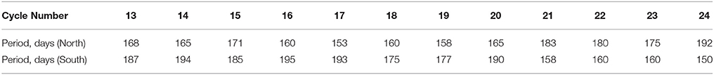
Table 1. Estimated Rieger periods (days) for northern and southern hemispheres from GRO sunspot area data for solar cycles 13–24.

The wavelet analysis confirms recent results of Gurgenashvili et al. (2016, 2017) that the Rieger-type periodicity depends on activity strength and the stronger activity displays shorter periodicity. For example, the northern hemisphere was more active during cycles 14–20, and consequently the corresponding wavelet analysis shows shorter periods of 155–165 days. After the cycle 21, when the northern hemisphere became weaker, the periods grew up to 175–190 days. The opposite dynamics is seen in the southern hemisphere. The longer periodicities about 190–195 days are observed during the cycles 13–20, while the period is shortened during the cycles 21–24, when the southern hemisphere became stronger. Red curves on the bottom panel of both figures display the fit of calculated Rieger-type periodicity over cycles. It is clearly seen that the periodicity is anti-correlated with the long term evolution of solar cycle strength in both hemispheres. Therefore, the Rieger-type periodicity is clearly magnetic strength dependent and it is probably related with the internal dynamo layer. However, a proper physical mechanism of the periodicity is needed in order to make the estimation of dynamo magnetic field strength. Here the Rossby waves appear to have interesting consequences.

3. Rossby Waves

Rossby waves arise owing to the conservation of absolute vorticity in rotating fluids. Therefore, inclusion of magnetic field has important influence spliting the hydrodynamic (HD) Rossby waves into fast and slow modes (Zaqarashvili et al., 2007). On the other hand, to study the Rossby waves in magnetohydrodynamic (MHD) approach is obviously more complicated. The dispersion relation of Rossby waves also significantly depend on angular velocity of rotating sphere and it is mostly controlled by the parameter

$\begin{array}{ll}ϵ=\frac{{\Omega }^2{R}^2}{gH},& (1)\end{array}$

where Ω is the angular velocity, R is the distance from the center to a shallow layer, g is the gravity and H is the layer thickness. Here gH is the square of surface gravity speed of the shallow layer. When ϵ ≪ 1 then the Rossby waves can be considered on spherical surface, which significantly simplifies the solution. On the other hand, when ϵ ≫ 1, which means either fast rotation or small surface gravity speed, then the waves in shallow layer can be trapped near the equator (Longuet-Higgins, 1968), but the solution is very complicated. Here we consider the both limits separately for the conditions of the tachocline.

3.1. Spherical Rossby waves

In the first case, we consider (θ, ϕ) surface over the sphere in the rotating frame with the toroidal magnetic field in the form B_θsinθ. In the simplest case of homogeneous magnetic field, B_θ = B₀, the Fourier analysis of linear MHD equations with exp(−iωt + mϕ), where ω is the wave frequency and m is the toroidal wavenumber, allows exact solutions in terms of associated Legendre polynomials

$\begin{array}{ll}{u}_{\theta }~P_n^m(\text{cos }\theta ),& (2)\end{array}$

where n is an integer and corresponds to a poloidal wavenumber. The exact dispersion relation for the spherical magneto-Rossby waves can be obtained as (Zaqarashvili et al., 2007)

$\begin{array}{ll}{\omega }_{nm}^2+\frac{2m\Omega }{n(n+1)}{\omega }_{nm}+\frac{m^2{\upsilon }_A^2}{R^2}\left(\frac{2}{n(n+1)}-1\right)=0,& (3)\end{array}$

where ${\upsilon }_A=B_0/\sqrt{4\pi \rho }$ is the Alfvén speed. Fast and slow magneto-Rossby waves are described by the expression

$\begin{array}{ll}{\omega }_{nm}=-\frac{m\Omega }{n(n+1)}\left(1\pm \sqrt{1-\frac{{\upsilon }_A^{2}n(n+1)}{{\Omega }^2{R}^2}(2-n(n+1))}\right).& (4)\end{array}$

The spatial structure of spherical magnetic Rossby waves for m = 1 and n = 3 (n = 4) harmonics is shown on the Figures 3, 4. In both cases the poloidal velocity is stronger on higher latitudes. If we take m = 1, n = 3 harmonic with the magnetic field of 10 kG, then the period of fast magneto-Rossby waves is 150 days and the period of slow magneto-Rossby waves is 6.3 years. n = 4 harmonics for the same field strength gives the period of 226 days for fast magneto-Rossby waves and 4 years for slow magneto-Rossby waves. For the stronger magnetic field with 100 kG n = 3 (n = 4) harmonic of the fast wave has the period of 47 days (52 days) and that of the slow wave has the period of 71 days (63 days). Therefore, the magnetic field strength of the order of 10 kG, which is an equipartition value of magnetic pressure in the tachocline with the overlying convection, gives nice correspondence with observed periodicity.

FIGURE 3

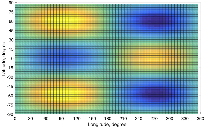
Figure 3. Spatial structure of spherical magneto-Rossby waves. Here the poloidal velocity of m = 1 and n = 3 harmonic is shown.

FIGURE 4

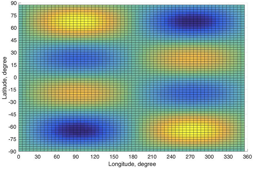
Figure 4. Spatial structure of spherical magneto-Rossby waves. Here the poloidal velocity of m = 1 and n = 4 harmonic is shown.

For the magnetic profile of B_θ = B₀cosθ, the Fourier analysis of linear MHD equations leads to the spheroidal wave equation for the weak magnetic field limit. The solutions are prolate spheroidal wave functions (S_nm(cosθ)) and the corresponding dispersion relation is

$\begin{array}{ll}{\omega }_{nm}^2+\frac{2m\Omega }{n(n+1)}{\omega }_{nm}-\frac{m^2{\upsilon }_A^2}{R^2}=0.& (5)\end{array}$

Fast and slow magneto-Rossby waves are described by the expression

$\begin{array}{ll}{\omega }_{nm}=-\frac{m\Omega }{n(n+1)}\left(1\pm \sqrt{1+\frac{{\upsilon }_A^2}{{\Omega }^2{R}^2}{n}^2{(n+1)}^2}\right).& (6)\end{array}$

For m = 1, n = 3 harmonic with the maximal magnetic field strength of 10 kG (this value is estimated taking into account the latitudinal profile of magnetic field, while B₀ = 20 kG in this case), the period of fast magneto-Rossby waves is 130 days and the period of slow magneto-Rossby waves is 1.7 years. n = 4 harmonics for the same field strength gives the period of 170 days for fast magneto-Rossby waves and 1.3 years for slow magneto-Rossby waves. Here we see that with the equipartition field strength, the m = 1, n = 4 harmonic of fast magneto-Rossby waves gives the value of Rieger-type periodicity, while the same harmonic of slow magneto-Rossby waves gives the similar value of annual oscillation (McIntosh et al., 2017). It is remarkable that the period exactly equals to the periodicity obtained by helioseismology near the base of convection zone (Howe et al., 2000). It is very interesting to study if this coincidence is just occasional or has a real physical ground.

3.2. Equatorial Waves

We consider the solar tachocline as a shallow layer with thickness H (~ 10⁹ cm) located at the distance R (~ 5 · 10¹⁰ cm) from the solar center (Spiegel and Zahn, 1992). We consider a local Cartesian frame (x, y, z) on rotating Sun, where x is directed toward west (i.e., in the direction of solar rotation), y is directed toward north, and z is directed vertically outwards. We adopt solid body rotation with the angular velocity –Ω = 2.6 × 10⁻⁶ s⁻¹. Differential rotation is neglected at this stage for two reasons. First, the value of differential rotation is small near the equator. Second, the differential rotation is of importance for instabilities and it will not significantly affect wave dispersion relations.

The sub-adiabatic temperature gradient in the upper part of the tachocline provides a negative buoyancy force to the deformed upper surface, therefore the surface feels less gravitational field compared to the real gravity (Gilman, 2000). The negative buoyancy force is proportional to the fractional difference between actual and adiabatic temperature gradients |∇ − ∇_ad|, which is in the range of 10⁻⁴−10⁻⁶ in the upper overshoot part of the tachocline and may reach up to 10⁻¹ in the lower radiative part of the tachocline (Dikpati and Gilman, 2001). Then the dimensionless value of reduced gravity G = 1/ϵ = gH/(R²Ω²) is proportional to $10^3|\nabla -{\nabla }_{ad}|$, therefore it is in the range of G > 100 in the radiative part of the tachocline and in the range of 10⁻³ ≤ G ≤ 10⁻¹ in the upper overshoot part (Dikpati and Gilman, 2001).

Magnetic field of the tachocline may obviously influence the dynamics of shallow layer, but the solutions for equatorial trapped HD shallow water waves are also very important at the first stage. These solutions can be found elsewhere (Matsuno, 1966; Lou, 2000), but we will study their properties in the tachocline conditions. We use equatorial β-plane approximation, which means to retain only the first order term in the expansion of Coriolis parameter near the equator, f = βy, where

$\begin{array}{ll}\beta =\frac{2\Omega }{R}.& (7)\end{array}$

Then the equation governing the linear dynamics of HD shallow water system is

$\begin{array}{ll}\frac{d^2{u}_y}{d{y}^2}+\left[\frac{{\omega }^2}{c^2}-k_x^2+\frac{k_x\beta }{\omega }-\frac{{\beta }^2}{c^2}{y}^2\right]u_y=0.& (8)\end{array}$

This is the equation of parabolic cylinder (also known as the equation of quantum harmonic oscillator) and when

$\begin{array}{ll}\frac{{\omega }^2}{c^2}-k_x^2+\frac{k_x\beta }{\omega }=\frac{\beta }{c}(2n+1)& (9)\end{array}$

then it has bounded solutions

$\begin{array}{ll}{u}_y=C\exp \left[-\frac{\beta }{c}\frac{y^2}{2}\right]H_n\left(\sqrt{\frac{\beta }{c}}y\right),& (10)\end{array}$

where H_n is the Hermite polynomial of order n and C is a constant. The solutions are oscillatory inside the interval

$\begin{array}{ll}y<\left|\sqrt{\frac{c}{\beta }(2n+1)}\right|& (11)\end{array}$

and exponentially tend to zero outside.

Equation (11) shows that the waves are trapped near the equator only for small $c=\sqrt{gH}$ and n. Therefore, in order to have equatorially trapped shallow water waves one needs very small surface gravity speed i.e., very small reduced gravity, G. This means that the waves can be trapped near the equator only in the upper overshoot part of the tachocline, where the reduced gravity is very small. In the lower radiative part of the tachocline the reduced gravity is still large, therefore the shallow water waves can not be trapped near the equator, but rather penetrate to higher latitudes and give the similar results those of the previous subsection. Therefore, in this subsection we will consider only the upper overshoot layer of the tachocline, where the reduced gravity is very small and hence it creates excellent conditions for the trapping of shallow water waves near the equator.

Equation (9) defines the dispersion relation for equatorial HD waves (see also Lou, 2000)

$\begin{array}{ll}{\omega }^3-\left[k_x^2{c}^2+\beta c(2n+1)\right]\omega +k_x\beta c^2=0.& (12)\end{array}$

From this equation it is immediately seen that the reduced gravity implies very low frequency waves for larger wavelengths with the dispersion relation

$\begin{array}{ll}\omega \approx \frac{k_{x}c}{2n+1},& (13)\end{array}$

which correspond to Rossby waves. The important point is that here the Rossby waves depend on the surface gravity speed, which was not the case in the previous subsection.

The discriminant of the cubic equation, $4{\left[k_x^2{c}^2+\beta c(2n+1)\right]}^3-27k_x^2{\beta }^2{c}^4$, is positive for entire range of k_x and c when n ≥ 1 and hence the equation has three real solutions

$\begin{array}{ll}{\omega }_j=2\sqrt{-\frac{p}{3}}\text{cos }\left[\frac{1}{3}\arccos \left(\frac{3q}{2p}\sqrt{-\frac{3}{p}}\right)-\frac{2\pi j}{3}\right]& (14)\end{array}$

where $p=-k_x^2{c}^2-\beta c(2n+1)$, $q=k_x\beta c^2$ and j = 0, 1, 2. The three solutions correspond to eastward propagating Rossby waves and two westward and eastward propagating Poincare waves plotted on Figure 5. Here the non-dimensional wavenumber k_xR is in the range of 1–5. The initial value of k_xR = 1 corresponds to the wavelength of 2πR and hence to the m = 1 harmonic in spherical coordinates, which has higher possibility to be excited. One can see from Figure 5 that the Rossby and Poincare waves have very different time scales. Figure 6 shows the dependence of Rossby waves on the value of normalized reduced gravity, G, for the wavenumber of k_xR = 1. When the gravity reaches the value of G = 0.001 − 0.0005 which is still reasonable for the overshoot layer, then the time scale of HD Rossby waves approaches to that of solar cycle, i.e., tens of years. This is a very interesting result which shows that solar cycle period can be obtained owing to equatorial Rossby waves in the case of temperature stratification of solar tachocline (or more correctly upper overshoot region). However, in order to make any connection of Rossby waves to solar cycles, the magnetic field should be inevitably involved.

FIGURE 5

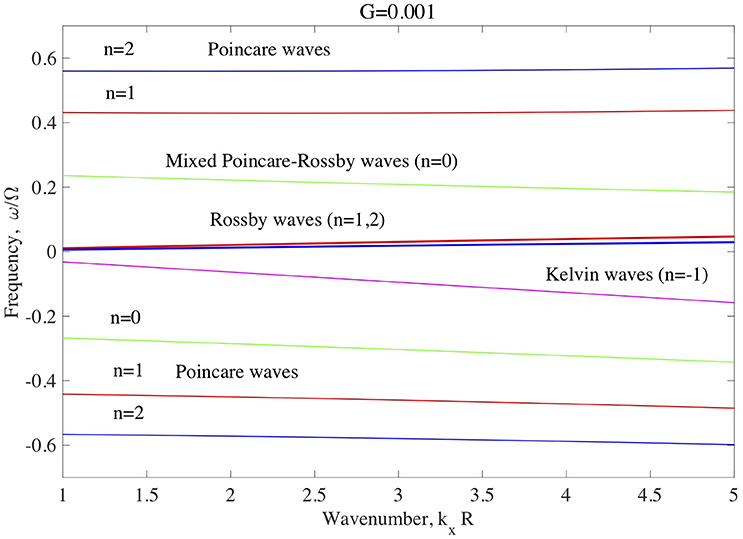
Figure 5. Dispersion curves for various equatorial HD shallow water waves in the solar tachocline. Red and blue thin solid lines correspond to eastward (positive) and westward (negative) propagating Poincare waves. Red and Blue thick solid lines correspond to eastward propagating Rossby waves. Green solid lines correspond to eastward propagating n = 0 mixed Poincare-Rossby waves and westward propagating n = 0 Poincare waves. Magenta solid line corresponds to Kelvin waves. Here the normalized value of the reduced gravity is G = 0.001.

FIGURE 6

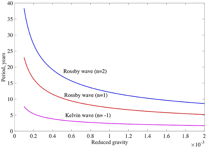
Figure 6. Period of equatorial HD Rossby and Kelvin waves vs. the value of normalized reduced gravity, G. Red and blue lines correspond to n = 1 and n = 2 Rossby wave harmonics, respectively. Magenta line corresponds to HD Kelvin waves. Here the harmonics with the wavenumber of k_xR = 1 are shown.

3.2.1. Poincare-Rossby Waves with n = 0

Equation (12) needs particular treatment for n = 0 mode, which has non-oscillatory structure with y direction. In this case it can be factorized as

$\begin{array}{ll}(\omega -k_{x}c)({\omega }^2+k_{x}c\omega -\beta c)=0.& (15)\end{array}$

The first zero ω = k_xc leads to the spurious solutions as the velocity perturbations become infinite in the initial equations. Consequently, n = 0 case has only two solutions: westward propagating Poincare wave and eastward propagating Poincare-Rossby wave (thin green solid lines on Figure 5, see detailed treatment in Matsuno, 1966).

For the small reduced gravity approximation, large-scale (in the toroidal direction) Poincare and Poincare-Rossby waves with n = 0 are described by the dispersion relation

$\begin{array}{ll}\omega =\pm \sqrt{\beta c},& (16)\end{array}$

which for G = 0.001 − 0.0001 gives the periods of 107–190 days. Therefore, the mixed Poincare-Rossby waves with n = 0 resemble the time scale of Rieger-type periodicity. Figure 7 displays the dependence of Poincare waves on the value of reduced gravity.

FIGURE 7

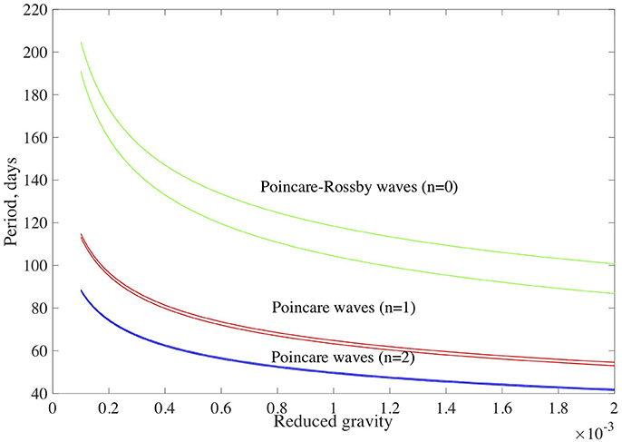
Figure 7. Period of equatorial Poincare waves vs. the value of normalized reduced gravity, G. Red and blue lines correspond to n = 1 and n = 2 Poincare wave harmonics, respectively. Green lines correspond to n = 0 mixed Poincare-Rossby waves. Here the harmonics with the wavenumber of k_xR = 1 are plotted.

In the case of n = 0 mode, a simple solution can be found in the presence of a homogeneous toroidal magnetic field, B₀. Near the equator the Equation (8) is now replaced by the equation (Zaqarashvili et al., 2007)

$\begin{array}{ll}\frac{d^2{u}_y}{d{y}^2}+\left[\frac{{\omega }^2-k_x^2{\upsilon }_A^2}{c^2}-k_x^2+\frac{k_x\beta \omega }{{\omega }^2-k_x^2{\upsilon }_A^2}-\frac{{\beta }^2{\omega }^2}{c^2({\omega }^2-k_x^2{\upsilon }_A^2)}{y}^2\right]u_y=0.& (17)\end{array}$

As u_y is not oscillatory along y, the bounded solution $~exp\left[-\beta |\omega |y^2/\left(2c\sqrt{{\omega }^2-k_x^2{\upsilon }_A^2}\right)\right]$ leads to the dispersion relation

$\begin{array}{ll}({\omega }^2-k_x^2{\upsilon }_A^2)(\sqrt{{\omega }^2-k_x^2{\upsilon }_A^2}+k_{x}c)-\beta c|\omega |=0.& (18)\end{array}$

For large-scale waves (small k_x) the dispersion relation can be approximated as

$\begin{array}{ll}\omega ~\pm \sqrt{\beta c+k_x^2{\upsilon }_A^2}.& (19)\end{array}$

3.2.2. Kelvin Waves

Particular class of waves arise when northward component of velocity (u_y) is zero. HD shallow water equations are rewritten as

$\begin{array}{ll}\frac{\partial u_x}{\partial t}=-g\frac{\partial h}{\partial x},& (20)\end{array}$

$\begin{array}{ll}\frac{\partial h}{\partial t}+H\frac{\partial u_x}{\partial x}=0,& (21)\end{array}$

$\begin{array}{ll}f{u}_x=-g\frac{\partial h}{\partial y}.& (22)\end{array}$

The Fourier expansion of Equations (20–21) with exp(iωt+ik_xx) leads to the dispersion relation

$\begin{array}{ll}(\omega -c{k}_x)(\omega +c{k}_x)=0,& (23)\end{array}$

which yields two different modes. The solutions for each mode can be easily found from Equation (22) as

$\begin{array}{ll}{u}_x=u_0\exp \left(\frac{1}{2}\frac{\beta }{c}{y}^2\right)& (24)\end{array}$

for ω = ck_x mode and

$\begin{array}{ll}{u}_x=u_0\exp \left(-\frac{1}{2}\frac{\beta }{c}{y}^2\right)& (25)\end{array}$

for ω = −ck_x mode. It is seen that the first solution does not satisfy boundary condition, therefore it is ruled out from the consideration. Hence, only the mode with the dispersion relation

$\begin{array}{ll}\omega =-c{k}_x& (26)\end{array}$

remains as the solution for Kelvin waves (see Figure 5).

This solution also arises from the dispersion relation, Equation (12), if one substitutes n = −1. Therefore, this mode was called as n = −1 mode by Matsuno (1966). The time scale of Kelvin waves is few years (see Figure 6), therefore it is in the range of quasi biennial (Sakurai, 1979; Zaqarashvili et al., 2010b) and/or annual oscillations (McIntosh et al., 2015, 2017).

The analysis of HD shallow water waves in the tachocline conditions show three different time scales, which actually correspond to observed variations in solar activity. It is interesting that the Rossby waves now have the time-scale which resembles solar cycles rather than Rieger-type oscillation. The Rieger-type periodicity now is better explained by equatorial Poincare-Rossby waves (n = 0). The tachocline magnetic field will surely modify the dispersion relations, but some preliminary estimations still can be done.

4. Seismology of Solar Dynamo Layer

Observed Rieger-type periodicities and dispersion relations of Rossby or Poincare-Rossby waves can be used to estimate the magnetic field strength in the tachocline. First we use the dispersion relation (Equation 6) of spherical fast magneto-Rossby wave (m = 1, n = 4 harmonics) and the observed periodicities from Table 1. The magnetic field is estimated for the cycles 13–24 in the northern and southern hemispheres separately. The resulted field strength is summarized on Table 2. It is clearly seen that the more active hemisphere possesses the strong magnetic field of >40 kG even in weaker cycles. On the other hand, less active hemisphere possesses weaker field of <40 kG even in the generally strong cycles. This result leads to two main conclusions. First, the dynamo magnetic field strength is more than 30 kG in all cycles, which means that the dynamo models with tachocline better explain the solar cycles than those without tachocline (see discussion in Gurgenashvili et al., 2016). Second, the result may mean that the strength of individual cycles is determined by the mutual interaction of oscillations in hemispheric magnetic fields rather than by the magnetic field strength itself. Therefore, the estimation using spherical Rossby wave scenario supports the results of McIntosh et al. (2015), who supposed that the solar cycles can be explained by the interactions of hemispheric activity bands.

TABLE 2

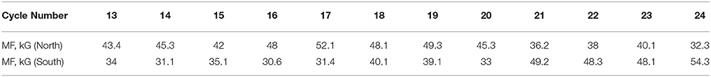
Table 2. Estimated magnetic field strength (kG) using spherical Rossby waves for northern and southern hemispheres from GRO sunspot area data for solar cycles 13–24.

On the other hand, n = 0 equatorial Poincare-Rossby waves can be also invoked in the estimation of the dynamo field strength. Using the dispersion relation, Equation (19), one can estimate the hemispheric toroidal magnetic field strength for solar cycles 13–24. The result is summarized on Table 3. Now the magnetic field strength in more active hemisphere is >20 kG even in weak cycles and <15 kG in the less active hemisphere even in strong cycles. Therefore, the field strength estimated by equatorial Poincare-Rossby waves is much less (almost three times) than that of estimated by spherical Rossby waves.

TABLE 3

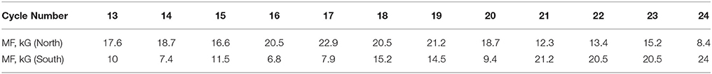
Table 3. Estimated magnetic field strength (kG) using equatorial Poincare-Rossby waves for northern and southern hemispheres from GRO sunspot area data for solar cycles 13–24.

Estimated field strength in the dynamo layer significantly depends on the excitation process of Rieger-type periodicities, therefore future detailed study may shed light in this important problem.

5. Discussion and Conclusions

Solar 11-year activity cycles are generally interpreted by some sort of solar dynamo, but exact model explaining all properties of solar magnetic field is not yet determined. Different dynamo models claim different locations and strengths of amplified magnetic field. The models are generally divided into two main groups: with and without tachocline. The models of first group consider the location of dynamo layer in the tachocline, just below the solar convection zone, where the magnetic field is amplified by the differential rotation and emerges on the solar surface as sunspots. The surface magnetic field is then carried toward poles by meridional circulation creating the poloidal component for the next cycle (Dikpati et al., 2004). The models of the second group consider the location of dynamo layer somewhere in (or throughout) the convection zone and the cyclic magnetic field is amplified due to turbulent (or say α²) processes (Tobias, 2009). The important difference between the models is the supposed strength of amplified magnetic field, which is much stronger in tachocline models (>20 kG) than in the models without tachocline (<10 kG). Therefore, even rough estimation of dynamo magnetic field might test the models.

Recently it was shown that the Rieger-type periodicity has strong dependence on solar activity level (Gurgenashvili et al., 2016), therefore it should be strongly linked to the dynamo layer in the solar interior. The periodicity then can be used to estimate the dynamo magnetic field strength and hence to test the dynamo models. Here we analyzed the Greenwich Royal Observatory hemispheric sunspot area data during cycles 13–24 by Morlet wavelet tool and found the Rieger-type periodicity in each cycle on both hemispheres separately. Our results again showed that the Rieger periodicity has shorter values (155–165 days) in more active hemisphere even in weak cycles and longer values (175–190 days) in less active hemisphere even in stronger cycles. The periods are summarized on Table 1.

Then the dispersion relations of Rossby-type waves were used to estimate the magnetic field strength in the dynamo layer. First, we showed that m = 1, n = 4 spherical harmonic of fast magneto-Rossby waves over spherical surface might be responsible for the Rieger-type periodicity. Corresponding dispersion relation gave the magnetic field strength of >40 kG in more active hemisphere also in weak cycles and <40 kG in less active hemisphere also in strong cycles. The estimated magnetic field strength during cycles 13–24 is presented on Table 2. Then, we showed that equatorial HD Poincare-Rossby waves (with n = 0), which are trapped near the equator owing to the reduced gravity in the upper overshoot tachocline, gave the Rieger-type periodicity. Considering preliminary magnetically affected dispersion relation, we estimated the magnetic field of >20 kG in more active hemispheres and <15 kG in less active hemispheres. The estimated magnetic field strength during cycles 13–24 is presented on Table 3. The estimations by equatorial Poincare-Rossby waves gave the magnetic field strength which is almost three times less than that of obtained by spherical fast magneto-Rossby waves. While the spherical Rossby waves fully support the models with tachocline, the equatorial Poincare-Rossby waves still keep the place for the models without tachocline as they estimate the field strength of <10 kG at least in the weaker hemisphere. Velocity field of spherical Rossby waves is concentrated more in higher latitudes and consists mostly in vortical structures, those number along latitude depends on the value of n. But, velocity field of equatorial Poincare-Rossby waves with n = 0 is concentrated in lower latitudes and consists in elliptic motion around the equator (see Figure 6b in Matsuno, 1966). Therefore, helioseismology in principle may test velocity fields of both spherical Rossby and equatorial Poincare-Rossby waves. On the other hand, both spherical and equatorial Rossby-type waves show that the solar cycles might be resulted from mutual interaction of hemispheric activity bands as suggested by McIntosh et al. (2015). Future detailed analytical, numerical and observational studies of Rossby-type waves are necessary to increase the accuracy of magnetic field estimation and to reveal the most plausible models for solar activity cycles.

Author Contributions

TZ wrote the sections 1,3,4,5 and prepared the Figures 3–7. EG wrote the sections 2, 4 and prepared the Figures 1, 2.

Funding

This work was funded by the Austrian Science Fund (FWF, projects P25181-N27 and P30695-N27) and by the Georgian Shota Rustaveli National Science Foundation project 217146.

Conflict of Interest Statement

The authors declare that the research was conducted in the absence of any commercial or financial relationships that could be construed as a potential conflict of interest.

Acknowledgments

This paper resulted from discussions at the workshop of ISSI (International Space Science Institute) team (ID 389) “Rossby waves in astrophysics” organized in Bern (Switzerland).

References

Carbonell, M., and Ballester, J. L. (1990). A short-term periodicity near 155 day in sunspot areas. Astron. Astrophys. 238, 377–381.

Google Scholar

Charbonneau, P. (2005). Dynamo Models of the Solar Cycle. Living Rev. Sol. Phys. 2:2. doi: 10.12942/lrsp-2005-2.

CrossRef Full Text | Google Scholar

Dikpati, M., and Gilman, P. A. (2001). Analysis of Hydrodynamic Stability of Solar Tachocline Latitudinal Differential Rotation using a Shallow-Water Model. Astrophys. J. 551, 536–564. doi: 10.1086/320080

CrossRef Full Text | Google Scholar

Dikpati, M., de Toma, G., Gilman, P. A., Arge, Ch. N., and White, O. R. (2004). Diagnostics of Polar Field Reversal in Solar Cycle 23 Using a Flux Transport Dynamo Model. Astrophys. J. 601, 1136–1151. doi: 10.1086/380508

CrossRef Full Text | Google Scholar

Dikpati, M., Cally, P. S., McIntosh, S. W., and Heifetz, E. (2017). The Origin of the “Seasons” in Space Weather. Nat. Sci. Rep. 7:14750. doi: 10.1038/s41598-017-14957-x

PubMed Abstract | CrossRef Full Text | Google Scholar

Gill, A. E. (1982). Atmosphere-Ocean Dynamics. San Diego, CA: Academic Press.

Google Scholar

Gilman, P. A. (2000). Magnetohydrodynamic “Shallow Water” equations for the Solar Tachocline. Astrophys. J. 544, L79–L82. doi: 10.1086/317291

CrossRef Full Text | Google Scholar

Gurgenashvili, E., Zaqarashvili, T. V., Kukhianidze, Oliver, R., Ballester, J. L., Ramishvili, G., et al. (2016). Rieger-type periodicity during solar cycles 14-24: estimation of dynamo magnetic field strength in the solar interior. Astrophys. J. 826:55. doi: 10.3847/0004-637X/826/1/55

CrossRef Full Text | Google Scholar

Gurgenashvili, E., Zaqarashvili, T. V., Kukhianidze, Oliver, R., Ballester, J. L., Dikpati, M., et al. (2017). North-south asymmetry in rieger-type periodicity during solar cycles 19-23. Astrophys. J. 845:137. doi: 10.3847/1538-4357/aa830a

CrossRef Full Text | Google Scholar

Howe, R., Christensen-Dalsgaard, J., Hill, F., Komm, R. W., Larsen, R. M., Schou, J., et al. (2000). Dynamic variations at the base of the solar convection zone. Science 287, 2456–2460. doi: 10.1126/science.287.5462.2456

PubMed Abstract | CrossRef Full Text | Google Scholar

Longuet-Higgins, M. S. (1968). The eigenfunctions of laplace's tidal equations over a sphere. Proc. R. Soc. Lond. A. 262, 511–607. doi: 10.1098/rsta.1968.0003

CrossRef Full Text

Lou, Y. Q. (2000). Rossby-type wave-induced periodicities in flare activities and sunspot areas or groups during solar maxima. Astrophys. J. 540, 1102–1108. doi: 10.1086/309387

CrossRef Full Text | Google Scholar

McIntosh, S. W., Leamon, R. J., Krista, L. D., Title, A. M., Hudson, H. S., Riley, P., et al. (2015). The solar magnetic activity band interaction and instabilities that shape quasi-periodic variability. Nat. Commun. 6:6491. doi: 10.1038/ncomms7491

PubMed Abstract | CrossRef Full Text | Google Scholar

McIntosh, S. W., Cramer W. J., Marcano, M. P., and Leamon, R. J. (2017). The detection of Rossby-like waves on the Sun. Nature Astron. 1:0086. doi: 10.1038/s41550-017-0086

CrossRef Full Text | Google Scholar

Matsuno, T. (1966). Quasi-Geostrophic motions in the equatorial area. J. Meteorol. Soc. Jpn. 44, 25–42.

Google Scholar

Oliver, R., Ballester, J. L., and Boudin, F. (1998). Emergence of magnetic flux on the Sun as the cause of a 158-day periodicity in sunspot areas. Nature 394, 552–553. doi: 10.1038/29012

CrossRef Full Text | Google Scholar

Rieger, E., Share, G. H., Forrest, D. J., Kanbach, G., Reppin, C., and Chupp, E. L. (1984). A 154-day periodicity in the occurrence of hard solar flares? Nature 312, 623–625. doi: 10.1038/312623a0

CrossRef Full Text | Google Scholar

Rossby, C.-G. (1939). Relation between variations in the intensity of the zonal circulation of the atmosphere and the displacements of the semipermanent centers of action. J. Marine Res. 2, 38–54

Google Scholar

Sakurai, K. (1979). Quasi-biennial variation of the solar neutrino flux and solar activity. Nature 278, 146–148. doi: 10.1038/278146a0

CrossRef Full Text | Google Scholar

Schwabe, M. (1844). Sonnenbeobachtungen im Jahre 1843. Von Herrn Hofrath Schwabe in Dessau. Astron. Nachrichten 21:233.

Google Scholar

Spiegel, E. A., and Zahn, J.-P. (1992). The solar tachocline. Astron. Astrophys. 265, 106–114.

Google Scholar

Tobias, S. M. (2009). The solar dynamo: the role of penetration, rotation and shear on convective dynamos. Space Sci. Rev. 144, 77–86. doi: 10.1007/s11214-008-9442-0

CrossRef Full Text | Google Scholar

Torrence, C., and Compo, G. P. (1998). A practical guide to wavelet analysis. Bull. American Met. Soc. 79, 61–78. doi: 10.1175/1520-0477(1998)079

CrossRef Full Text | Google Scholar

Zaqarashvili, T. V., Oliver, R., Ballester, J. L., and Shergelashvili, B. M. (2007). Rossby waves in “shallow water” magnetohydrodynamics. Astron. Astrophys. 470, 815–820. doi: 10.1051/0004-6361:20077382

CrossRef Full Text | Google Scholar

Zaqarashvili, T. V., Carbonell, M., Oliver, R., and Ballester, J. L. (2010a). Magnetic Rossby Waves in the Solar Tachocline and Rieger-Type Periodicities. Astrophys J., 709, 749-758. doi: 10.1088/0004-637X/709/2/749

CrossRef Full Text | Google Scholar

Zaqarashvili, T. V., Carbonell, M., Oliver, R., Ballester, J. L. (2010b). Quasi-biennial oscillations in the solar tachocline caused by magnetic rossby wave instabilities. Astrophys. J. 724, L95–L98. doi: 10.1088/2041-8205/724/1/L95

CrossRef Full Text | Google Scholar