On Mass Spectra of Primordial Black Holes

1 Introduction

Interest in the primordial black holes (PBHs) is dramatically increasing since the gravitational waves discovery from the black holes mergers (Abbott, 2016). However, PBHs origin and possible formation mechanisms are still a topical issue of modern astrophysics and cosmology. The first ideas of such mechanisms had been proposed in (Zel’dovich and Novikov, 1967; Hawking, 1971; Carr and Hawking, 1974) and lately developed in many other works (see reviews and references within (Khlopov, 2010; Carr et al., 2020; Carr and Kühnel, 2020)). The different PBH spectra are used in papers (Carr, 1975; Dolgov and Silk, 1993; Sendouda et al., 2006; Clesse and García-Bellido, 2015; Garriga et al., 2016; Carr and Kühnel, 2019; Liu et al., 2020) depending on specific needs.

The phase transitions of the first (Hawking et al., 1982; Kodama et al., 1982; Konoplich et al., 1998; Jedamzik and Niemeyer, 1999; Konoplich et al., 1999) and the second order (Rubin et al., 2000; Rubin et al., 2001) might also underlay a mechanism of the PBH formation. In this paper, we continue elaboration of the model based on the second type phase transitions during the inflationary epoch (Rubin et al., 2000; Rubin et al., 2001; Khlopov et al., 2002). However, the described model has a flaw. It inevitably leads to a multiple production of small mass PBHs. That problem could not be avoided within the framework of the discussed scenario, and typical mass spectra have the falling form d N/d M ∝ M^−α, α > 0 (see review (Belotsky et al., 2019)). Such a form of spectra could be unfavorable for explaining the observable effects. In addition, the overproduction of low-mass PBHs could contradict future experiments.

The solution to the above problems is to use the classical motion of massive scalar fields together with their quantum fluctuations. The idea was firstly studied in (Dokuchaev et al., 2010) to suppress the production of intermediate-mass black holes. In this research, we have elaborated this idea and obtain the analytical formula for the field distribution probability.

At present, there are a lot of models that contain a complicated form of scalar field potential. The latter is used in a variety of inflationary models predicting the potential landscape. In addition, inflation can be driven by the dynamics of several fields (Wands et al., 2007). For instance, the supergravity often produces more than one physical scalar field (Ketov and Starobinsky, 2012) and predicts nontrivial forms of inflaton potentials (Ketov, 2021). The string theory also predicts the landscape with a large number of vacua, local peaks, and saddle points (Susskind, 2003; Cline, 2005). Such a complex potential can have both random and quasi-periodic forms (Li et al., 2009) and leads to the multi-field inflation such as multi-stream one (Li and Wang, 2009; Duplessis et al., 2012), assisted inflation (Battefeld and Battefeld, 2009) or multi-field inflation with a random potential (Tye et al., 2009; Frazer and Liddle, 2012). Therefore, other non-inflaton scalar fields might have complicated potential as well.

In this paper, we adopt the mechanism of black hole formation (Rubin et al., 2000; Rubin et al., 2001; Khlopov et al., 2002; Belotsky et al., 2019) to the modern trends in the inflaton potential complication. A complex potential shape influences the classical motion of the fields so that the analytical form of the probability contains the classical trajectories as well as the quantum field contributions. The resulting black holes mass spectrum appears to be related to a shape of the scalar field’s potential. The tool elaborated here allows fixing the potential form by knowledge of black hole mass distribution.

This paper is organized as follows. In Section 2, we elaborate the way to involve the classical part of scalar fields into the expression for its fluctuations probability. The PBH spectrum depends on an initial position of the scalar field that allows us to adjust the model predictions to future observational data without inserting small parameters. The numerical results are represented in Section 3. Finally, Section 4 concludes the paper.

2 Quantum Fluctuations Accompanied by Classical Motion at the Inflationary Stage

The discussed mechanism of PBHs production requires closed domain walls formation due to the quantum fluctuations of scalar fields at the inflation epoch (Rubin et al., 2000; Rubin et al., 2001). Let us take into account both the quantum and classical motion of fields. Consider the scalar field Φ of mass m and the standard action

$S=\frac{M_{\text{Pl}}^2}{2}\int {\mathrm{d}}^{4}x\sqrt{g_4}\left[R+{\left(\partial \mathrm{\Phi }\right)}^2-m^2{\mathrm{\Phi }}^2\right].(1)$

Here, M_Pl is the Planck mass. The scalar field could be the inflaton field as well as a spectator one. The field equation in the de Sitter space is represented as (Khlopov and Rubin, 2004)

$\begin{array}{l}\hfill \frac{\partial \mathrm{\Phi }}{\partial t}-\frac{1}{3H}\left[e^{-2Ht}\mathrm{\Delta }\mathrm{\Phi }-\frac{\partial V\left(\mathrm{\Phi }\right)}{\partial \mathrm{\Phi }}\right]=y\left(\mathbf{x},t\right);\\ \hfill y\left(\mathbf{x},t\right)\equiv \left(-\frac{1}{3H}\frac{{\partial }^2}{\partial t^2}-\frac{\partial }{\partial t}+\frac{1}{3H}{e}^{-2Ht}\mathrm{\Delta }\right)Q\left(\mathbf{x},t\right).\end{array}(2)$

Here, Q (x, t) is the “quick” part of the Fourier field decomposition. This equation was simplified: we have omitted the second time derivative due to a slow roll approximation and have neglected higher powers of the function y (x, t). The latter is supposed to be small so that we may find a solution to the equation in the form

$\mathrm{\Phi }={\mathrm{\Phi }}_{\text{cl}}+\varphi .(3)$

The deterministic part of the classical field Φ_cl is governed by the equation

$\frac{\partial {\mathrm{\Phi }}_{\text{cl}}}{\partial t}-\frac{1}{3H}\left[e^{-2Ht}\mathrm{\Delta }{\mathrm{\Phi }}_{\text{cl}}-\frac{\partial V\left({\mathrm{\Phi }}_{\text{cl}}\right)}{\partial {\mathrm{\Phi }}_{\text{cl}}}\right]=0,(4)$

while its random part ϕ depends strictly on quantum fluctuations according to the linear equation

$\frac{\partial \varphi }{\partial t}-\frac{1}{3H}\left[e^{-2Ht}\mathrm{\Delta }\varphi -V^{″}\left({\mathrm{\Phi }}_{\text{cl}}\right)\varphi \right]=y\left(\mathbf{x},t\right).(5)$

Here, we consider the limit Φ_cl ≫ ϕ which is valid if the random “force” y (x, t) is small. Let us denote

$m^2\left(t\right)\equiv V^{″}\left({\mathrm{\Phi }}_{\text{cl}}\right).(6)$

The parameter m is positive if we are near the bottom of potential and is imaginary if we are near the potential maximum. It is supposed that m(t) varies slowly during inflation.

We are interested in the super horizon scales where the fluctuations do not depend on the space coordinates. The uniform distribution Φ = Φ(t) is governed by the more simple equation

$\frac{\partial {\mathrm{\Phi }}_{\text{cl}}}{\partial t}+\frac{1}{3H}\frac{\partial V\left({\mathrm{\Phi }}_{\text{cl}}\right)}{\partial {\mathrm{\Phi }}_{\text{cl}}}=0,(7)$

$\frac{\partial \varphi }{\partial t}+\mu \left(t\right)\varphi =y\left(t\right);\mu \left(t\right)\equiv \frac{m^2\left(t\right)}{3H},(8)$

provided that H(t) = const. The correlator of the random function y(t) may be approximated as follows (Rey, 1987)

$⟨y\left(t_1\right)y\left(t_2\right)⟩=D\left(\mathbf{x},t_1;\mathbf{x},t_2\right)=\frac{H}{4{\pi }^2}\delta \left(t_1-t_2\right).(9)$

The delta function in the rhs of this expression indicates that the random function y(t) is distributed according to the Gauss law with the density

$W\left(y\right)=\mathrm{const}\exp \left[-\frac{1}{2{\sigma }^2}\int y^2\left(t\right)\mathrm{d}t\right],\sigma =\frac{H^{3/2}}{2\pi }.(10)$

The probability distribution of the function ϕ is proportional to that of the function y(t) due to their linear relationship (8). It means that the probability to find the specific value ϕ(t) inside some small interval is equal to (Feynman et al., 2010)

$\mathrm{d}P\left(\varphi \right)=\mathrm{const}\mathcal{D}\varphi \exp \left[-\frac{1}{2{\sigma }^2}\int {\left[\frac{\partial \varphi }{\partial t}+\mu \left(t\right)\varphi \right]}^2\mathrm{d}t\right].(11)$

Let’s obtain the probability to find a quantum part of the field ϕ₂ at an instant t₂ provided that a value ϕ₁ at an instant t₁ is known. Evidently, we have to integrate over all values of the field inside the interval (t₁, t₂) and come to the expression

$\mathrm{d}P\left({\varphi }_2,t_2;{\varphi }_1,t_1\right)=\mathrm{const}\mathrm{d}{\varphi }_2\underset{{\varphi }_1}{\overset{{\varphi }_2}{\int }}\mathcal{D}\varphi \exp \left[-\frac{1}{2{\sigma }^2}\underset{t_1}{\overset{t_2}{\int }}{\left[\frac{\partial \varphi }{\partial t}+\mu \left(t\right)\varphi \right]}^2\mathrm{d}t\right].(12)$

The constant factor in this equation is determined by normalization condition

$\underset{-\infty }{\overset{\infty }{\int }}\frac{\mathrm{d}P\left({\varphi }_2,t_2;{\varphi }_1,t_1\right)}{\mathrm{d}{\varphi }_2}\mathrm{d}{\varphi }_2=1.(13)$

Functional integral (12) can be calculated in the standard manner by finding an extreme trajectory of the integral in the exponent

$\ddot{\varphi }-{\mu }^2\left(t\right)\varphi =0,(14)$

where the term $\dot{\mu }$ is neglected due to slow variation of μ(t). The boundary conditions for (14) are as follows

$\varphi \left(t_1\right)={\varphi }_1;\varphi \left(t_2\right)={\varphi }_2.(15)$

Exact solution to this equation is

$\varphi \left(t\right)=A\exp \left(M\left(t\right)\right)+B\exp \left(-M\left(t\right)\right);M\left(t\right)\equiv \underset{t_1}{\overset{t}{\int }}\mu \left(t^{\prime }\right)\mathrm{d}{t}^{\prime };(16)$

$A=\frac{{\varphi }_2-{\varphi }_1{e}^{-M\left(t_2\right)}}{2\sinh \left(M\left(t_2\right)\right)},B=-\frac{{\varphi }_2-{\varphi }_1{e}^{M\left(t_2\right)}}{2\sinh \left(M\left(t_2\right)\right)}.(17)$

Notice that M(t₁) = 0 by definition.

Substituting this solution into the integral in the exponent of the expression (12) one obtains the desired probability in the saddle point approximation

$\begin{array}{ll}\hfill \mathrm{d}P\left({\varphi }_2,t_2;{\varphi }_1,t_1\right)& =\mathrm{const}\mathrm{d}{\varphi }_2\exp \left[-\frac{2A^2}{{\sigma }^2}\underset{t_1}{\overset{t_2}{\int }}{\mu }^2\left(t\right)e^{2M\left(t\right)}\mathrm{d}t\right]\hfill \\ \hfill & =\mathrm{const}\mathrm{d}{\varphi }_2\exp \left[-q^2{\left({\varphi }_2-{\varphi }_1{e}^{-M\left(t_2\right)}\right)}^2\right],\hfill \end{array}(18)$

$q^2\equiv \frac{1}{2{\sigma }^2{\sinh }^2\left(M\left(t_2\right)\right)}\underset{t_1}{\overset{t_2}{\int }}{\mu }^2\left(t\right)e^{2M\left(t\right)}\mathrm{d}t.(19)$

It describes the probability to find specific value of “quantum” part of the field (3). The “classical” part of the field Φ_cl is incorporated into the function M(t). The probability for the field value F (the distribution function f) is easily obtained by substitution ϕ(t) = Φ(t) − Φ_cl(t) into the formula above.

$\begin{array}{ll}\hfill f\left({\mathrm{\Phi }}_2,t\right)& =\frac{\mathrm{d}P\left({\mathrm{\Phi }}_2,t;{\mathrm{\Phi }}_1,t_1\right)}{\mathrm{d}{\mathrm{\Phi }}_2}\hfill \\ \hfill & =\sqrt{\frac{q^2}{\pi }}\exp \left[-q^2{\left({\mathrm{\Phi }}_2-{\mathrm{\Phi }}_{\text{cl}}\left(t_2\right)-\left({\mathrm{\Phi }}_1-{\mathrm{\Phi }}_{\text{cl}}\left(t_1\right)\right)e^{-M\left(t_2\right)}\right)}^2\right].\hfill \end{array}(20)$

The limit m → 0 restores the textbook formula.

The next section aims to demonstrate how the obtained formulas can be applied to a particular scalar field potential. It is assumed that the potential may possess many extremes of a different kind. In our consideration, we choose a part of phase space containing two maxima and at least one saddle point.

3 The PBH Formation

In this section, we show that the classical motion of fields together with their quantum fluctuations influence the PBH mass spectra. To this end, we have to find the classical trajectory and use the probability (20) derived above.

The fields move between potential local maxima that lead to complicated spectra of fluctuations. The latter are discussed in papers (Wands et al., 2007; Ketov and Starobinsky, 2012). At the same time, the presence of saddle points is the reason for the closed domain walls formation, see details in (Gani et al., 2018; Murygin et al., 2021). In the following, they could collapse to black holes (Rubin et al., 2001; Belotsky et al., 2019).

Let us consider the model of two real scalar fields with the Lagrangian

$\mathcal{L}=\frac{1}{2}\left({\partial }_{\mu }\mathrm{\Phi }{\partial }^{\mu }\mathrm{\Phi }+{\partial }_{\mu }\mathrm{X}{\partial }^{\mu }\mathrm{X}\right)-V\left(\mathrm{\Phi },\mathrm{X}\right).(21)$

We choose the potential possessing n peaks and saddle points

$\begin{array}{c}V\left(\mathrm{\Phi },\mathrm{X}\right)=\frac{m_{\varphi }^2}{2}{\mathrm{\Phi }}^2+\frac{m_{\chi }^2}{2}{\mathrm{X}}^2+\sum _{i=1}^n\delta V_i\left(\mathrm{\Phi },\mathrm{X}\right),\\ \delta V_i\left(\mathrm{\Phi },\mathrm{X}\right)={\mathrm{\Lambda }}_i^4\exp \left(-{\left(\frac{\mathrm{\Phi }-{\varphi }_i}{{\mathrm{\Delta }}_i}\right)}^2-{\left(\frac{\mathrm{X}-{\chi }_i}{{\mathrm{\Delta }}_i}\right)}^2\right).\end{array}(22)$

Here, δV_i describes the ith local maximum. The global minimum of the potential is located at the point (ϕ_min, χ_min) = (0, 0) with exponentially small errors. Hereinafter, all variables are taken in the Hubble units H where H ≈ 10¹³ GeV at the inflationary epoch.

For our estimates, we choose the fields masses m_ϕ = 0.4 and m_χ = 0.5. For simplicity, we consider the potential with two peaks (n = 2) with the coordinates ϕ₁ = − 9.0, χ₁ = 3.0 and ϕ₂ = − 1.7, χ₂ = 4.5. The parameters corresponding to the peaks heights are Λ₁ = 3.0 and Λ₂ = 1.5, and the peaks widths are set with Δ₁ = 0.5 and Δ₂ = 1.5. The initial fields values are ϕ_in = − 8.0 and χ_in = 45.0. Note, all chosen parameters have the values $\sim \mathcal{O}(1)$.

Following Section 2, the first step consists of finding the classical trajectory Φ_cl(t), X_cl(t) of the fields Φ, X. Starting from the initial values (ϕ_in, χ_in) at the inflation epoch, the scalar fields tend to the potential minimum. The process is described by the classical motion equations

$\left\{\begin{array}{c}{\mathrm{\Phi }}_{\text{cl},tt}+3H{\mathrm{\Phi }}_{\text{cl},t}+\frac{\partial V\left({\mathrm{\Phi }}_{\text{cl}},{\mathrm{X}}_{\text{cl}}\right)}{\partial {\mathrm{\Phi }}_{\text{cl}}}=0,\hfill \\ {\mathrm{X}}_{\text{cl},tt}+3H{\mathrm{X}}_{\text{cl},t}+\frac{\partial V\left({\mathrm{\Phi }}_{\text{cl}},{\mathrm{X}}_{\text{cl}}\right)}{\partial {\mathrm{X}}_{\text{cl}}}=0.\hfill \end{array}\right.(23)$

The classical evolution of the fields and the form of the specific potential are shown in Figure 1. At the same time, quantum fluctuations lead to fields “diffusion” during inflation. The probability density f to find the fields F or X in any point of the physical space is given by (20).

FIGURE 1

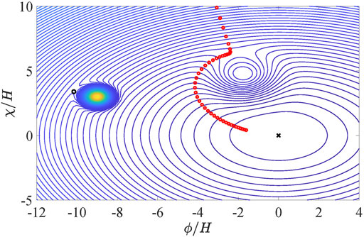
FIGURE 1. The contour plot of the potential (22) with the parameters m₁=0.4, m₂=0.5, Λ₁=3.0, Λ₂=1.5, ϕ₁=−9.0, χ₁=3.0, ϕ₂=−1.7, χ₂=4.5, Δ₁=0.5, Δ₂=1.5 is shown. The red circles illustrate the classical trajectory of the fields Φ, X, and the black cross shows the potential minimum. The initial fields values for (23) are ϕ_in =−8.0 and χ_in =45.0.

Both F and X distributions depend on a classical position of the fields at the instant t. In our estimates, we suppose that the probability function for the quantum parts ϕ or χ of the fields is separated into two independent fluctuation processes

$f\left(t,\varphi ,\chi \right)=f_{\varphi }\left(t,\varphi \right)f_{\chi }\left(t,\chi \right)=\frac{\mathrm{d}P}{\mathrm{d}\varphi }\frac{\mathrm{d}P}{\mathrm{d}\chi },(24)$

where distribution functions of each field ϕ, χ can be defined as in (18).

As noted above, the fields should reach a saddle point of potential for domain wall formation. Suppose that some quantum fluctuation crosses a saddle point and ends up at a point of the area O. As was shown in (Gani et al., 2018; Murygin et al., 2021), it causes nontrivial field solutions of the system (23) characterized by a nonzero winding number. Such configurations might lead to the domain walls formation after the inflation is finished. Detailed explanation might be found in (Gani et al., 2018). The calculation of an exact shape of the area O is a separate, quite complicated task, so that we limit ourselves with the following approximation. Let us assume that the area O is bordered by two lines χ_cl-sp(Φ) and χ_{min  −sp}(Φ) in the phase space. The first line connects the classical value at the instant t and the saddle point (ϕ_sp, χ_sp)

${\chi }_{\text{cl}-\text{sp}}\left(\mathrm{\Phi }\right)={\chi }_{\text{sp}}+\frac{\mathrm{\Phi }-{\varphi }_{\text{sp}}}{{\varphi }_{\text{cl}}\left(t\right)-{\varphi }_{\text{sp}}}\left({\chi }_{\text{cl}}\left(t\right)-{\varphi }_{\text{sp}}\right).(25)$

The second one connects the vacuum value and the saddle point

${\chi }_{\min -\text{sp}}\left(\mathrm{\Phi }\right)={\chi }_{\text{sp}}+\frac{\mathrm{\Phi }-{\varphi }_{\text{sp}}}{{\varphi }_{\min }-{\varphi }_{\text{sp}}}\left({\chi }_{\min }-{\varphi }_{\text{sp}}\right).(26)$

Thus, the probability for the fields to attain the area O where domain walls might form is calculated by integrating (24)

$P\left(t\right)=\underset{\mathrm{\Omega }}{\int \int }f\left(\varphi ,\chi ,t\right)\mathrm{d}\mathrm{X}\mathrm{d}\mathrm{\Phi }=\underset{{\varphi }_{\text{sp}}}{\overset{+\infty }{\int }}{f}_{\varphi }\left(\varphi ,t\right)\mathrm{d}\mathrm{\Phi }\underset{{\chi }_{\text{cl}-\text{sp}}\left(\mathrm{\Phi }\right)}{\overset{{\chi }_{\min -\text{sp}}\left(\mathrm{\Phi }\right)}{\int }}{f}_{\chi }\left(\chi ,t\right)\mathrm{d}\mathrm{X}.(27)$

Here, both distribution functions f_ϕ and f_χ are defined in (20) and according to (3) ϕ = Φ − Φ_cl, χ = X − X_cl. The algorithm for calculating the probability (27) discussed above is more accurate then that used in the previous papers.

Now, let us find the mass spectra of primordial black holes. In the considered model, they are formed due to the collapse of domain walls. Here, we briefly reproduce the idea, while details may be found in the review (Belotsky et al., 2019). As was shown in (Gani et al., 2018; Murygin et al., 2021), domain walls might be formed due to the quantum fluctuations in field models with potential possessing at least one saddle point and a local maximum. The proto-soliton is formed if the fields achieve a saddle point (in our model, we have noted this area as Ω). These proto-soliton field configurations are quickly expanded during inflation. The final scale of such configuration depends on an e-fold number N. More definitely, the configuration scale is stretched in the factor $\sim e^{N_{\inf }-N}$ to the end of inflation. The soliton is quickly formed after the end of inflation. The total mass of the field configuration is proportional to its area. It could collapse into a black hole after the end of inflation (Rubin et al., 2000; Rubin et al., 2001; Khlopov et al., 2002).

The regions number where the fields reach the critical values ϕ_cr and χ_cr belonging to O can be found as

$n\left(t\right)=P\left(t\right)e^{3Ht}.(28)$

Here, the term e^3Ht is the number of causally independent regions of the size H⁻¹ at the instant t from the beginning of inflation. After the end of inflation at t = N_infH⁻¹ = 60H⁻¹, the size of each region is expanded

$r_0\left(t\right)=H^{-1}\exp \left(N_{\inf }-Ht\right)\gg r_{h,0}.(29)$

Here, N_inf ≈ 60 is the total e-folds number, and r_h,0 is the horizon size at the end of inflation. At the radiation stage (RD), each region expands as $\propto \sqrt{\tau }$ while the horizon size is r_h = H⁻¹(τ) = 2τ. Here, τ is time after the beginning of the RD epoch. After a domain wall goes under the horizon, its collapse begins (the details of the process taking into account detachment from the Hubble flow may be found in (Khlopov et al., 2005; Dokuchaev et al., 2008; Belotsky et al., 2019)). Thus, the maximal size of a domain wall can be written as the function of the instant t

$r\left(t\right)\approx \frac{1}{2}\frac{e^{2\left(N_{\inf }-Ht\right)}}{H{N}_{\inf }}.(30)$

After eliminating of t from (28) and 30, one can finally get the distribution n(r) of closed walls sizes which can be rearranged into the mass spectrum.

Next, we have to find masses of PBHs. For simplicity, we assume total energy of domain wall converts to a black hole mass during its collapse and neglect nonsphericity of a domain wall and losses caused by gravitational waves. The energy density of a domain wall might be found by a common way. The energy momentum tensor for the Lagrangian (21) is given by

$T_{\nu }^{\mu }=\sum _{i=\mathrm{1,2}}\left({\partial }^{\mu }{\phi }_i{\partial }_{\nu }{\phi }_i-\frac{1}{2}{\partial }^{\alpha }{\phi }_i{\partial }_{\alpha }{\phi }_i{\delta }_{\nu }^{\mu }\right)+V{\delta }_{\nu }^{\mu },(31)$

where φ₁, φ₂ correspond to the fields Φ_cl and X_cl, respectively. Then, the energy density of a domain wall is found to be

$\epsilon \left(x\right)=T_0^0=\frac{1}{2}\sum _{i=\mathrm{1,2}}\left({\left({\partial }_t{\phi }_i\right)}^2+{\left({\partial }_x{\phi }_i\right)}^2\right)+V.(32)$

Upon integrating (32) over the all possible values of x (infinite interval), the surface energy density of a domain wall σ may be found. Finally, masses of black holes are $M\left(r(t)\right)\simeq 4\pi \sigma r^2(t)$. Taking into account (28) and (30), one can find the mass spectrum of primordial black holes. The PBH mass distribution for the parameters of the Lagrangian (21) is shown in Figure 2. Note, the mass spectrum has the non-power form due to taking into account both the quantum and classical motion of scalar fields and the compound form of the potential leading to nontrivial classical fields trajectory. The obtained spectrum is free from the overproduction of light PBHs and, therefore, is much more adaptable to new observational effects. We leave a detailed analysis of these possibilities for future research.

FIGURE 2

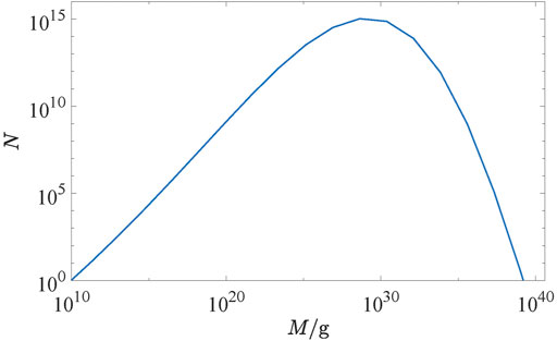
FIGURE 2. The PBH mass distribution is shown.

4 Conclusion

In this note, we have shown that the mechanism of PBHs formation in the second-order phase transitions of scalar fields might produce a wide variety of the PBH mass spectra. It is expected that observations (e.g. cosmic gamma-rays, gravitational waves spectrum (Sakharov et al., 2021), gravitational lensing (Toshchenko and Belotsky, 2019)) will help to select an appropriate one. The key point is the classical field motion which was taken into account together with the quantum fluctuations at the inflationary stage. We show here that the probability to find a particular value of the scalar field at a space point depends on its classical dynamics. We have derived the appropriate analytical formula and have applied it to obtain one of the PBH mass spectra. The elaborated method is the useful tool to fit an observable spectrum in the near future.

Data Availability Statement

The original contributions presented in the study are included in the article/supplementary materials, further inquiries can be directed to the corresponding author.

Author Contributions

A. Kirillov is responsible for the mass spectrum calculation (Section 3) and S. Rubin is responsible for the probability derivation in Section 2.

Conflict of Interest

The authors declare that the research was conducted in the absence of any commercial or financial relationships that could be construed as a potential conflict of interest.

The reviewer AS declared a past co-authorship with one of the authors SR to the handling editor.

Publisher’s Note

All claims expressed in this article are solely those of the authors and do not necessarily represent those of their affiliated organizations, or those of the publisher, the editors and the reviewers. Any product that may be evaluated in this article, or claim that may be made by its manufacturer, is not guaranteed or endorsed by the publisher.

Acknowledgments

The work of AK was funded by the Ministry of Science and Higher Education of the Russian Federation, Project “Fundamental properties of elementary particles and cosmology” 0723-2020-0041. The work of SR has been supported by the Kazan Federal University Strategic Academic Leadership Program.

References

Abbott, B. P. (2016). Observation of Gravitational Waves from a Binary Black Hole Merger. Phys. Rev. Lett. 116, 061102. doi:10.1103/PhysRevLett.116.061102

PubMed Abstract | CrossRef Full Text | Google Scholar

Battefeld, D., and Battefeld, T. (2009). Multi-field Ination on the Landscape. J. Cosmol. Astropart. Phys. 2009, 027. doi:10.1088/1475-7516/2009/03/027

CrossRef Full Text | Google Scholar

Belotsky, K. M., Dokuchaev, V.I., Eroshenko, Y. N., Esipova, E. A., Khlopov, M. Y., Khromykh, L. A., et al. (2019). Clusters of Primordial Black Holes. Eur. Phys. J. C 79, 246. doi:10.1140/epjc/s10052-019-6741-4

CrossRef Full Text | Google Scholar

Carr, B., Kohri, K., Sendouda, Y., and Yokoyama, J. (2020). Constraints on Primordial Black Holes. arXiv e-prints. arXiv:2002.12778 [astro-ph.CO].

Google Scholar

Carr, B. J., and Hawking, S. W. (1974). Black Holes in the Early Universe. Mon. Not. R. Astron. Soc. 168, 399–416. doi:10.1093/mnras/168.2.399

CrossRef Full Text | Google Scholar

Carr, B. J. (1975). The Primordial Black Hole Mass Spectrum. Astrophys. J. 201, 1–19. doi:10.1086/153853

CrossRef Full Text | Google Scholar

Carr, B., and Kühnel, F. (2020). Primordial Black Holes as Dark Matter: Recent Developments. Annu. Rev. Nucl. Part. Sci. 70, 355–394. doi:10.1146/annurev-nucl-050520-125911

CrossRef Full Text | Google Scholar

Carr, B., and Kühnel, F. (2019). Primordial Black Holes with Multimodal Mass Spectra. Phys. Rev. D 99, 103535. doi:10.1103/physrevd.99.103535

CrossRef Full Text | Google Scholar

Clesse, S., and García-Bellido, J. (2015). Massive Primordial Black Holes from Hybrid Ination as Dark Matter and the Seeds of Galaxies. Phys. Rev. D 92, 023524. doi:10.1103/physrevd.92.023524

CrossRef Full Text | Google Scholar

Cline, J. M. (2005). Ination from String Theory. arXiv e-prints. arXiv:0501179 [hep-th].

Google Scholar

Dokuchaev, V. I., Eroshenko, Y. N., and Rubin, S. G. (2008). Early Formation of Galaxies Induced by Clusters of Black Holes. Astron. Rep. 52, 779–789. doi:10.1134/s1063772908100016

CrossRef Full Text | Google Scholar

Dokuchaev, V. I., Eroshenko, Y. N., Rubin, S. G., and Samarchenko, D. A. (2010). “Mechanism for the Suppression of Intermediatemass Black Holes. Astron. Lett. 36, 773–779. doi:10.1134/s1063773710110022

CrossRef Full Text | Google Scholar

Dolgov, A., and Silk, J. (1993). Baryon Isocurvature Uctuations at Small Scales and Baryonic Dark Matter. Phys. Rev. D 47, 4244–4255. doi:10.1103/physrevd.47.4244

PubMed Abstract | CrossRef Full Text | Google Scholar

Duplessis, F., Wang, Y., and Brandenberger, R. (2012). Multi-stream Ination in a Landscape. J. Cosmol. Astropart. Phys. 2012, 012. doi:10.1088/1475-7516/2012/04/012

CrossRef Full Text | Google Scholar

Feynman, R., Hibbs, A., and Styer, D. (2010). Quantum Mechanics and Path Inte- Grals, Dover Books on Physics. Mineola, NY, USA: Dover Publications.

Google Scholar

Frazer, J., and Liddle, A. R. (2012). Multi-field Ination with Random Potentials: Field Dimension, Feature Scale and Non-gaussianity. J. Cosmol. Astropart. Phys. 2012, 039. doi:10.1088/1475-7516/2012/02/039

CrossRef Full Text | Google Scholar

Gani, V. A., Kirillov, A. A., and Rubin, S. G. (2018). Classical Transitions with the Topological Number Changing in the Early Universe. J. Cosmol. Astropart. Phys. 2018, 042. doi:10.1088/1475-7516/2018/04/042

CrossRef Full Text | Google Scholar

Garriga, J., Vilenkin, A., and Zhang, J. (2016). Black Holes and the Multiverse. J. Cosmol. Astropart. Phys. 2016, 064. doi:10.1088/1475-7516/2016/02/064

CrossRef Full Text | Google Scholar

Hawking, S. (1971). Gravitationally Collapsed Objects of Very Low Mass. Mon. Not. R. Astron. Soc. 152, 75. doi:10.1093/mnras/152.1.75

CrossRef Full Text | Google Scholar

Hawking, S. W., Moss, I. G., and Stewart, J. M. (1982). Bubble Collisions in the Very Early Universe. Phys. Rev. D 26, 2681. doi:10.1103/physrevd.26.2681

CrossRef Full Text | Google Scholar

Jedamzik, K., and Niemeyer, J. C. (1999). Primordial Black Hole Formation during First-Order Phase Transitions. Phys. Rev. D 59, 124014. doi:10.1103/physrevd.59.124014

CrossRef Full Text | Google Scholar

Ketov, S. V. (2021). Multi-Field versus Single-Field in the Supergravity Models of Ination and Primordial Black Holes. Universe 7, 115. doi:10.3390/universe7050115

CrossRef Full Text | Google Scholar

Ketov, S. V., and Starobinsky, A. A. (2012). Ination and Nonminimal Scalarcurvature Coupling in Gravity and Supergravity. J. Cosmol. Astropart. Phys. 2012, 022. doi:10.1088/1475-7516/2012/08/022

CrossRef Full Text | Google Scholar

Khlopov, M. Y. (2010). Primordial Black Holes. Res. Astron. Astrophys 10, 495–528. doi:10.1088/1674-4527/10/6/001

CrossRef Full Text | Google Scholar

Khlopov, M. Y., and Rubin, S. G. (2004). Cosmological Pattern of Microphysics in the Inationary Universe. P.O. Box 17, 3300 AA Dordrecht, Netherlands: Kluwer Academic Publishers.

Google Scholar

Khlopov, M. Y., Rubin, S. G., and Sakharov, A. S. (2005). Primordial Structure of Massive Black Hole Clusters. Astropart. Phys. 23, 265–277. doi:10.1016/j.astropartphys.2004.12.002

CrossRef Full Text | Google Scholar

Khlopov, M. Y., Rubin, S. G., and Sakharov, A. S. (2002). Strong Primordial Inhomogeneities and Galaxy Formation. arXiv e-prints. arXiv:0202505 [astro-ph].

Google Scholar

Kodama, H., Sasaki, M., and Sato, K. (1982). Abundance of Primordial Holes Produced by Cosmological First Order Phase Transition. Prog. Theor. Phys. 68, 1979. doi:10.1143/ptp.68.1979

CrossRef Full Text | Google Scholar

Konoplich, R. V., Rubin, S. G., Sakharov, A. S., and Khlopov, M. Y. (1998). Formation of Black Holes in first-Order Phase Transitions in the Universe. Astron. Lett. 24, 413–417.

Google Scholar

Konoplich, R. V., Rubin, S. G., Sakharov, A. S., and Khlopov, M. Y. (1999). Formation of Black Holes in First-Order Phase Transitions as a Cosmological Test of Symmetry-Breaking Mechanisms. Phys. Atom. Nucl. 62, 1593–1600.

Google Scholar

Li, M., and Wang, Y. (2009). Multi-stream Ination. J. Cosmol. Astropart. Phys. 2009, 033. arXiv:0903.2123 [hep-th]. doi:10.1088/1475-7516/2009/07/033

CrossRef Full Text | Google Scholar

Li, S., Liu, Y., and Piao, Y.-S. (2009). Ination in a Web. Phys. Rev. D 80, 123535. arXiv:0906.3608 [hep-th]. doi:10.1103/physrevd.80.123535

CrossRef Full Text | Google Scholar

Liu, J., Guo, Z.-K., and Cai, R.-G. (2020). Primordial Black Holes from Cosmic Domain walls. Phys. Rev. D 101, 023513. doi:10.1103/physrevd.101.023513

CrossRef Full Text | Google Scholar

Murygin, B. S., Kirillov, A. A., and Nikulin, V. V. (2021). Cosmological Formation of (2 + 1)-Dimensional Soliton Structures in Models Possessing Potentials with Local Peaks. Physics 3, 563–568. doi:10.3390/physics3030035

CrossRef Full Text | Google Scholar

Rey, S.-J. (1987). Dynamics of Inationary Phase Transition. Nucl. Phys. B 284, 706–728. doi:10.1016/0550-3213(87)90058-7

CrossRef Full Text | Google Scholar

Rubin, S. G., Khlopov, M. Y., and Sakharov, A. S. (2000). Primordial Black Holes from Non-equilibrium Second Order Phase Transition. Grav. Cosmol. S 6, 51–58. arXiv:hep-ph/0005271.

Google Scholar

Rubin, S. G., Sakharov, A. S., and Khlopov, M. Y. (2001). The Formation of Primary Galactic Nuclei during Phase Transitions in the Early Universe. J. Exp. Theor. Phys. 92, 921–929. doi:10.1134/1.1385631

CrossRef Full Text | Google Scholar

Sakharov, A. S., Eroshenko, Y. N., and Rubin, S. G. (2021). Looking at the NANOGrav Signal through the Anthropic Window of Axionlike Particles. Phys. Rev. D 104, 043005. doi:10.1103/physrevd.104.043005

CrossRef Full Text | Google Scholar

Sendouda, Y., Nagataki, S., and Sato, K. (2006). Mass Spectrum of Primordial Black Holes from Inationary Perturbation in the Randall Sundrum Braneworld: a Limit on Blue Spectra. J. Cosmol. Astropart. Phys. 2006, 003. doi:10.1088/1475-7516/2006/06/003

CrossRef Full Text | Google Scholar

Susskind, L. (2003). The Anthropic Landscape of String Theory. The davis Meet. cosmic ination, 26. arXiv:0302219 [hep-th].

Google Scholar

Toshchenko, K. A., and Belotsky, K. M. (2019). Studying Method of Microlensing Effect Estimation for a Cluster of Primordial Black Holes. J. Phys. Conf. Ser. 1390, 012087. doi:10.1088/1742-6596/1390/1/012087

CrossRef Full Text | Google Scholar

Tye, S.-H. H., Xu, J., and Zhang, Y. (2009). Multi-field Ination with a Random Potential. J. Cosmol. Astropart. Phys. 2009, 018. arXiv:0812. 1944 [hep-th].

CrossRef Full Text | Google Scholar

Wands, D. (2007). “Multiple Field Ination,” in Lect. Notes Phys. Editors M. Lemoine, J. Martin, and P. Peter (Berlin: Springer), Vol. 738, 275.

Google Scholar

Zel'dovich, Y. B., and Novikov, I. D. (1967). The Hypothesis of Cores Retarded during Expansion and the Hot Cosmological Model. Sov. Astron. J. 10, 602–603. doi:10.1070/pu1967v009n04abeh003014

CrossRef Full Text | Google Scholar