Theoretical Refinements to the Heliospheric Upwind eXtrapolation Technique and Application to in-situ Measurements

1 Introduction

Beyond 10–20 solar radii (R_S), plasma launched from the Sun travels along roughly radial trajectories. Temporal variations, likely driven by re-configurations of the coronal magnetic field, as well as the large-scale differential rotation of the Sun, conspire to place parcels of plasma of different speeds, densities, and temperatures along the same radial path [e.g., (Riley et al., 2012)]. Where faster material attempts to outrun slower material, compression fronts are created, whereas when fast material outruns slower material behind, an expansion wave (or rarefaction) forms [e.g., (Gosling and Pizzo, 1999)]. Particularly during the declining phase and at solar minimum, when transient activity (and coronal mass ejections in particular) is reduced, these processes produce large-scale corotating interaction regions (CIRs); global structures that appear to corotate with the Sun.

The structure and properties of these CIRs has been explored and reproduced with a reasonably-high degree of fidelity over the years with increasingly sophisticated numerical models [e.g. (Pizzo, 1978; Pizzo and Gosling, 1994; Riley et al., 2001; Riley et al., 2012; Shiota et al., 2014; Riley et al., 2019; Poedts et al., 2020; Poirier et al., 2020; Réville et al., 2020)]. However, such approaches are computationally expensive and generally require significant time investment by the user. Previously, we developed an extrapolation procedure, HUX (Heliospheric Upwinding eXtrapolation), which provided a simpler approach for reconstructing the structure of the inner heliosphere (out to distances where pick-up ions could be neglected) based on a simplification of the momentum equation. Riley and Lionello (Riley and Lionello, 2011) (“Paper 1”) introduced the HUX technique and demonstrated that it could reproduce MHD solutions with high accuracy (Pearson correlation coefficient, PCC ∼ 0.98). Riley and Issan (Riley and Issan, 2021) (“Paper 2”) extended the model to allow the user to map solar wind streams both outward (away from the Sun) and inward (back to the Sun); in both cases, the results being considerably more accurate than ballistic mapping solutions.

In this study, we further investigate the theoretical underpinnings of the HUX technique, as well as refinements to it. We also apply the technique to several solar wind datasets. Specifically, in Section 2 we summarize the main methodologies used, including models and data, while in Section 3 we focus on several theoretical considerations, including higher-order refinements to the HUX technique. In Section 4 we apply the refined HUX technique to in-situ measurements, mapping observed stream structure from one location to another and comparing it directly with observations from spacecraft at that location. Finally, in Section 5, we discuss the main points of this study, point out a few important caveats and limitations, and suggest how these results may be employed in future studies.

2 Methodology

2.1 Models

2.1.1 The HUX Technique

We consider three distinct model approximations here: (1) ballistic; (2) HUX; and (3) MHD. The so-called ballistic approximation simply states that a parcel of plasma maintains its speed throughout the region of interest, say, from 30R_S to 5 AU. This provides an exceedingly simple way to map the plasma to different locations in the heliosphere, assuming that it maintains a radial trajectory. In Supplementary Appendix A, we recover the ballistic approximation using the method of characteristics, and in Supplementary Appendix B, we derive an expression that defines where the characteristics intersect, and, hence, where the ballistic approximation fails.

The HUX approach, which represents a compromise between the ballistic and MHD approximations has been described in more detail in papers 1 and 2. Briefly, we begin by assuming that the large-scale evolution of the solar wind motion can be approximated by the fluid momentum equation in a corotating frame of reference (Pizzo, 1978; Riley and Lionello, 2011; Riley and Issan, 2021):

$-{\mathrm{\Omega }}_{\text{rot}}\frac{\partial \bar{v}}{\partial \varphi }+\left(\bar{v}\cdot \nabla \right)\bar{v}=\frac{1}{\rho }\nabla p-\frac{G{M}_s}{r^2}{\mathbf{e}}_r(1)$

where r is the radial distance from the Sun, ϕ is Carrington longitude in Heliographic (rotating) coordinate system (HG), θ is heliographic latitude, $\bar{v}=[v_{\varphi },v_{\theta },v_r]$ is the solar wind velocity, ρ(ϕ, θ, r) is the plasma density, p(ϕ, θ, r) is the plasma pressure, G is the gravitational constant, M_s is the solar mass, and Ω_rot(θ) is the angular frequency of the Sun’s rotation set equal to $\frac{2\pi }{25.38}\text{rads/day}$ at the solar equator, and more generally is a function of latitude (Riley and Issan, 2021). This last term, however, as we have shown previously, is unlikely to be important for mapping out solar wind streams (Riley and Issan, 2021), although it is worth noting that Parker Solar Probe (PSP) did observe substantial tangential solar wind speeds [e.g. (Finley et al., 2020)].

To progress further, as in Papers 1 and 2, we neglect the pressure gradient and gravity terms, and only consider variations of the velocity in the radial direction (Pizzo, 1978; Riley and Gosling, 1998). With these simplifications, the fluid momentum equation reduces to a two-dimensional non-linear scalar homogeneous time-stationary equation, described by:

$\frac{\partial v_r}{\partial \varphi }-\frac{1}{{\mathrm{\Omega }}_{\text{rot}}}{v}_r\frac{\partial v_r}{\partial r}=0(2)$

where the independent variables are r, ϕ and the dependent variable is v_r(ϕ, r). The initial-boundary value problem (IBVP) is defined by Eq. 2 on the domain 0 ≤ ϕ ≤ 2π and r ≥ 30R_S, where R_S denotes solar radii unit of distance.

The problem described by Eq. 2 is subject to the initial condition v_r(ϕ, r₀) with periodic boundary conditions, such that v_r(0, r) = v_r(2π, r) for all radial locations. Eq. 2 would be considered to be of the form of the well-studied inviscid Burgers’ equation, if the propagation was in the longitude direction; however, we advance in the radial direction. By solving Eq. 2 we aim to approximate the solar wind radial speed near Earth at 1AU ≈ 215R_S given an initial condition in the inner heliosphere, say, at 30R_S. Having defined the problem, we are now in the position to explore mathematical methods to solve our underlying equation (Eq. 2).

2.1.2 Acceleration Effects

Riley and Lionello (Riley and Lionello, 2011) proposed adding an ad hoc acceleration boost to the initial velocity profile near the Sun (approximately 30R_S to 50R_S) to account for residual acceleration of the solar wind. The acceleration boost is described by the following expression:

$v_{\text{acc}}\left(r\right)=\alpha \left[v_r\left(\varphi ,r_0\right)\right]\left(1-e^{-r/r_h}\right)(3)$

where v_r(ϕ, r₀) is the initial solar wind speed, α is the factor by which we increase the speed, and r_h is the span over which the acceleration lasts (Riley and Lionello, 2011). Essentially, α and r_h are free parameters, but which previously (papers 1 and 2) were found to be: α = 0.15 and r_h = 50R_S. Thus, for forward mapping, to account for the solar wind acceleration, we alter the initial velocity by adding v_acc before propagating the solution, while, for backward mapping, we first back-propagate then subtract the results at, say, 30R_S by v_acc.

2.2 Data

In this study, we initially surveyed a range of data from NASA’s Space Physics Data Facility (SPDF). These included the OMNI dataset, providing in-situ measurements of the plasma and magnetic field upstream of the Earth, as well as Helios 1 and 2, Voyagers 1 and 2, Pioneers 10 and 11, and Ulysses, which spanned a range of heliocentric distances, latitudes, and longitudes. However, as discussed more below, to reduce the likelihood that disagreements in the mapped and observed data were the result of the spacecraft sampling different plasma, we required that the two datasets being compared were substantially aligned in latitude at the time of the observation. This reduced the number of conjunctions to three: Helios 1 and 2 and OMNI.

The Helios mission was aimed at providing observations of the inner heliosphere region to gain a better understanding of solar wind evolution. Helios 1 and 2 were launched on December 10, 1974, and January 15, 1976, respectively, and Helios 1 continued to operate up to 1984 (Rosenbauer et al., 1977; Mariani et al., 1979; Schwenn and Marsch, 1990). On April 17 1976, at a distance of 0.29 AU, Helios 1 travelled closer to the Sun than any other previous spacecraft; a record that was not broken until October 29 2018 by Parker Solar Probe.

For this study, we used Helios data collected by the plasma experiment instrument, which measured the density, speed, and temperature of the solar wind (Rosenbauer et al., 1977). To download the data, we used HelioPy, a community-developed Python package for space physics (Stansby et al., 2021), which, in turn retrieved the data from NASA’s Space Physics Data Facility (SPDF) website (https://cdaweb.gsfc.nasa.gov/index.html/). We also used the Python package PsiPy to download PSI’s MAS (Magnetohydrodynamics Algorithm outside a Sphere) model results (Riley, 2021).

The OMNI dataset is an aggregation of data from multiple near-Earth spacecraft (primarily IMP 8, Geotail, Wind and ACE), providing solar wind measurements at Earth (King and Papitashvili, 2005). These data were also obtained from SPDF using the HelioPy interface.

3 Refinements to the HUX Technique

In this section, we introduce several explicit 2-level numerical methods to solve Eq. 2. Ideally, a sufficient numerical method is: (1) at least second-order accurate; (2) highly-accurate at discontinuities; and (3) absent of artificial oscillations (LeVeque, 1992). Before applying numerical methods to estimate derivatives, we rewrite Eq. 2 in hyperbolic conservation form as:

$\frac{\partial }{\partial r}{v}_r+\frac{\partial }{\partial \varphi }\left[f\left(v_r\right)\right]=0(4)$

The physical flux function is f(v_r) = − Ω_rotln(v_r) and because $f^{\prime \prime }(v_r)=\frac{{\mathrm{\Omega }}_{\text{rot}}}{{v_r}^2}>0\forall v_r>0$, f is said to be convex. When f′′(v_r) does not change sign, such in the model described here, discontinuous solutions appear in the form of either a shock or an expansion wave (LeVeque, 1992).

3.1 Convergence

Numerical methods are considered convergent, i.e., the numerical solution converges to the true solution, if the method is consistent and stable (LeVeque, 1992). To satisfy the consistency requirement, the numerical flux function should meet the following condition: If v_i,j = v_i,j+1, then $\mathcal{F}(v_{i,j},v_{i,j+1})=f(v_{i,j})$, where $\mathcal{F}$ and f denote the numerical and physical flux functions, respectively. Furthermore, for any numerical method to be considered stable, it must satisfy the Courant–Friedrichs–Lewy (CFL) condition as the grid is refined. The CFL condition states that the method’s numerical domain of dependence must contain the true domain of dependence of the equation (Courant et al., 1967). For Eq. 2 with the first-order upwind scheme, the CFL restriction is based on the grid cell and the domain of dependence, such that the following inequality must hold:

$\varphi -\mathrm{\Delta }\varphi \le \varphi -\frac{{\mathrm{\Omega }}_{\text{rot}}}{v_r}\left(\mathrm{\Delta }r\right)\le \varphi (5)$

More succinctly, the Courant number ν is restricted to be less than or equal to 1 to ensure stability¹:

$\nu =\frac{\mathrm{\Delta }r{\mathrm{\Omega }}_{\text{rot}}}{v_r\mathrm{\Delta }\varphi }(6)$

for 0 ≤ ν ≤ 1, where Δr can be dynamically modified as the method propagates the solution forward in the radial direction. Note that for higher order numerical methods, the Courant number has a more lenient tolerance.

3.2 First-Order Numerical Methods

The Heliospheric Upwind eXtrapolation Technqiue developed in paper 1 leverages the first-order upwind scheme in quasi-linear form to solve Eq. 2 numerically. The reasoning behind this is because we assume v_r > 0, ∀r, ϕ; therefore, the wave propagates only in one direction, the “upwind” direction. The HUX-f (forward) technique maps solar wind streams from the inner heliosphere ($\approx 30R_S$) to Earth (1 AU), such that:

${\mathbf{v}}_{i+1,j}={\mathbf{v}}_{i,j}+\frac{\mathrm{\Delta }r{\mathrm{\Omega }}_{\text{rot}}}{{\mathbf{v}}_{i,j}}\left(\frac{{\mathbf{v}}_{i,j+1}-{\mathbf{v}}_{i,j}}{\mathrm{\Delta }\varphi }\right)(7)$

where v denote the discretizion of v_r and the indices i and j refer to r and ϕ grids, respectively. In contrast, the HUX-b (backwards) technique, which is also based on the first-order upwind method, marches in the downwind direction, such that the mapping technique is applied to near-Earth data and mapped back to the Sun. The HUX-b method is defined as:

${\mathbf{v}}_{i-1,j}={\mathbf{v}}_{i,j}+\frac{\mathrm{\Delta }r{\mathrm{\Omega }}_{\text{rot}}}{{\mathbf{v}}_{i,j}}\left(\frac{{\mathbf{v}}_{i,j-1}-{\mathbf{v}}_{i,j}}{\mathrm{\Delta }\varphi }\right)(8)$

Although the first-order upwind method is simple and stable, it also results in smeared solutions near discontinuities, mimicking–in a crude sense–the effects of viscosity.

3.3 Higher-Order Numerical Methods

To overcome significant numerical dissipation that is associated with all first-order numerical methods, we now consider higher-resolution methods in an attempt to improve the standard HUX-f/b technique. The higher-resolution methods are at least second-order accurate in smooth regions yet still are easy to implement and computationally efficient.

3.3.1 MacCormack’s Method

The upwind method discussed in Section 3.2 is a first-order method. The MacCormack method is a higher-order method that uses first-order differencing and then backward differencing to achieve second-order accuracy (MacCormack, 1969). It is described by:

$\begin{array}{cc}\hfill {\tilde{\mathit{v}}}_{i,j}& ={\mathbf{v}}_{i,j}-\frac{\mathrm{\Delta }r}{\mathrm{\Delta }\varphi }\left[f\left({\mathbf{v}}_{i,j+1}\right)-f\left({\mathbf{v}}_{i,j}\right)\right]\hfill \\ \hfill {\mathbf{v}}_{i+1,j}& =\frac{1}{2}\left({\mathbf{v}}_{i,j}+{\tilde{\mathit{v}}}_{i,j}\right)-\frac{\mathrm{\Delta }r}{2\mathrm{\Delta }\varphi }\left[f\left({\tilde{\mathit{v}}}_{i,j}\right)-f\left({\tilde{\mathbf{v}}}_{i,j-1}\right)\right]\hfill \end{array}(9)$

It should be noted, however, that although the MacCormack method is highly accurate on smooth solutions, the method’s results exhibit artificial oscillations at discontinuities.

3.3.2 Richtmyer Two-step Lax-Wendroff Method

Similar to MacCormack’s method, the Richtmyer two-step Lax-Wendroff method is second-order accurate on smooth regions (LeVeque, 1992), and is based on the Taylor series expansion (LeVeque, 1992). The method is applied in two steps. The first step approximates the half steps as

${\mathbf{v}}_{i+1/2,j+1/2}=\frac{1}{2}\left({\mathbf{v}}_{i,j+1}+{\mathbf{v}}_{i,j}\right)-\frac{\mathrm{\Delta }r}{2\mathrm{\Delta }\varphi }\left[f\left({\mathbf{v}}_{i,j+1}\right)-f\left({\mathbf{v}}_{i,j}\right)\right];(10)$

Then, the second step computes the next full radial iteration, where:

${\mathbf{v}}_{i+1,j}={\mathbf{v}}_{i,j}-\frac{\mathrm{\Delta }r}{\mathrm{\Delta }\varphi }\left[f\left({\mathbf{v}}_{i+1/2,j+1/2}\right)-f\left({\mathbf{v}}_{i+1/2,j-1/2}\right)\right](11)$

Again, the Lax-Wendroff method suffers from artificial oscillations near discontinuities. Figure 1 illustrates the effects of implementing these second-order schemes. We make the following remarks. First, overall, both the first- and second-order schemes are able to map out the MHD solution reasonably well from 30R_S to 1 AU. Second, the second-order schemes seem to perform better in capturing the smaller scale structure, such as the oscillations in the slow solar wind from 0° to 120° longitude. Third, the higher-order approaches are able to maintain the amplitude of the high-speed streams better than the first-order approximation. Fourth, the higher-order schemes significantly overshoot the troughs between each of the high-speed streams. Fifth the higher-order schemes are better able to capture the rising gradients (rarefaction side) in the streams.

FIGURE 1

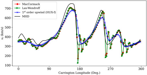
FIGURE 1. Comparison between 1^st-order upwind scheme (HUX-f), MacCormack method, and Lax Wendroff method versus the MHD solution. The initial solar wind data is at 30R_S, at the solar equator, and mapped out to 1AU.

3.4 Flux-Limiter Methods

First-order methods are total variation diminishing (TVD), meaning that they attempt to better capture shocks or discontinuities without introducing spurious oscillations, yet, they result in numerical dissipation. Higher-order methods result in better accuracy in smooth regions, but exhibit artificial oscillations near discontinuities. Flux-limiter methods aim to address both limitations. In regions of discontinuities, the flux-limiter method will behave as a low-order method, while in smooth regions, it chooses the higher-order approximation (LeVeque, 2002). The flux-limiter method depends on the wave gradient, such that:

$F\left({\mathbf{v}}_{i,j}\right)=F_L\left({\mathbf{v}}_{i,j}\right)+\mathrm{\Phi }\left[F_H\left({\mathbf{v}}_{i,j}\right)-F_L\left({\mathbf{v}}_{i,j}\right)\right](12)$

where Φ(v) is the limiter function, F_L is the numerical flux function of the first-order method (e.g. 1^st-order upwind scheme), and F_H is the numerical flux function of a higher-order method (e.g., MacCormack’s method). Near discontinuities, Φ is close to zero (F ∼ F_L), while in smooth regions Φ is approximately 1 (F ∼ F_H). There are multiple ways to measure the smoothness of the data, a common approach being to evaluate the gradient, Θ:

${\mathrm{\Theta }}_{i,j}=\frac{{\mathbf{v}}_{i,j}-{\mathbf{v}}_{i,j-1}}{{\mathbf{v}}_{i,j+1}-{\mathbf{v}}_{i,j}}(13)$

Some of the most common limiter functions used in the scientific literature are the “superbee” and “minmod” limiters developed by Roe, and the smooth limiter function and monotonized central (MC) function developed by Van Leer (Van Leer, 1974; Van Leer, 1977; LeVeque, 2002). These are defined by the following functions:

$\begin{array}{cc}\hfill {\mathrm{\Phi }}_{\text{Superbee}}\left(\mathrm{\Theta }\right)& =\max \left(0,\min \left(\mathrm{1,2}\mathrm{\Theta }\right),\min \left(\mathrm{\Theta },2\right)\right)\hfill \\ \hfill {\mathrm{\Phi }}_{\text{minmod}}\left(\mathrm{\Theta }\right)& =\max \left(0,\min \left(1,\mathrm{\Theta }\right)\right)\hfill \\ \hfill {\mathrm{\Phi }}_{\text{VanLeer}}\left(\mathrm{\Theta }\right)& =\frac{\mathrm{\Theta }+|\mathrm{\Theta }|}{1+|\mathrm{\Theta }|}\hfill \\ \hfill {\mathrm{\Phi }}_{\text{MC}}\left(\mathrm{\Theta }\right)& =\max \left(0,\min \left(\left(1+\mathrm{\Theta }\right)/\mathrm{2,2,2}\mathrm{\Theta }\right)\right)\hfill \end{array}(14)$

Figure 2 illustrates the improvement of flux-limiter methods from solely lower or higher-order methods. Many of the same points made for Figure 1 can be made when comparing the flux limiter techniques with the first-order upwind approach. More importantly, however, the major artifact that was introduced by the second-order approaches–the drop in speed between the high-speed streams–is now gone. The flux-limiter techniques have combined the best aspects from each of the earlier approaches.

FIGURE 2

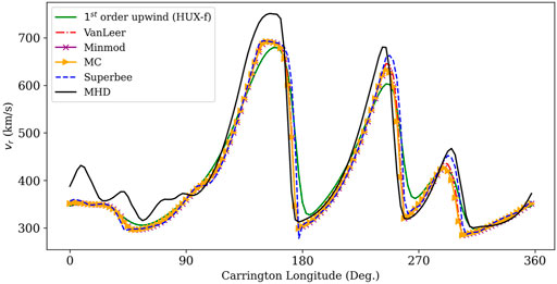
FIGURE 2. Comparison between limiter functions (Superbee, Van Leer, MC, and Minmod) and the 1st-order upwind scheme in the original HUX technique, with the “ground truth” MHD solution for CR 2210. The high and lower order methods used for the flux-limiter method is Lax-Wendroff and the 1st-order upwind scheme, respectively. The initial solar wind data is at 30R_S, at the solar equator, and mapped out to 1 AU.

Table 1 provides the mean squared error (MSE) and the pearson correlation coefficient (PCC) between flux-limiter numerical method schemes and the MHD solution for CR2210 at the solar equator after mapping from 30R_S to 1AU. For this time period, the MacCormack method coupled with first-order upwind method slightly out-performed the Lax-Wendroff coupled with the first-order upwind scheme. However, the difference was not significant. Among the four different limiter functions (Superbee, VanLeer, MC, and minmod), the minmod flux-limiter function resulted in the best fit, with the MacCormack method coupled with the first-order upwind scheme along with minmod flux-limiter function resulting in: PCC ∼ 0.966 and MSE ∼ 1599.0. All the flux functions showed improvement from the original HUX technique that used a first-order upwind scheme, and for which: PCC ∼ 0.921 and MSE ∼ 2581.8. Moreover, the flux limiter functions provides second-order accuracy in smooth regions, yet is as simple to implement and as computationally efficient as the original HUX technique. For standard HUX and flux-limiter methods, the average computation time was 0.03 and 0.3 s on a modest desktop CPU, respectively. In contrast, computing global MHD solutions for a full Carrington rotation requires several to many hours on a reasonably large multi-processor or GPU system (Riley et al., 2021).

TABLE 1

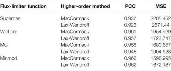
TABLE 1. A comparison of flux-limiter functions.

Finally, we remark that even more sophisticated high-order numerical methods exist, such as weighted essentially non-oscillatory (WENO) methods. Since the HUX technique is used primarily as a surrogate model for the 3-D MHD model, we have aimed to improve the accuracy of the HUX technique while retaining ease of use and computational efficiency. Thus, we suggest that improving the standard HUX technique by leveraging flux-limiter methods provides the optimum balance by: (1) accurately capturing shock formation; (2) achieving higher accuracy in smooth regions; and (3) avoiding severe numerical dissipation when mapping out to large heliocentric distances.

4 Mapping In-Situ Measurements Through the Heliosphere

Armed with this refined HUX (rHUX) technique we now apply it to in-situ measurements. We apply the Lax-Wendroff method coupled with the first-order upwind scheme along with the minmod flux-limiter function. As noted earlier, although there exist a large number of spacecraft datasets that we could potentially investigate, the requirement that the measurements be taken while the spacecraft are aligned in latitude, as well as over periods of relatively low solar activity, effectively limited the set to Helios 1 and 2 and Earth-based spacecraft (captured by the OMNI dataset). We begin by mapping Helios 1 measurements to Earth, then taking Earth measurements and mapping them to the location of Helios 1. Following this, we repeat the process using Helios 2 measurements.

4.1 Mapping From Helios 1 to OMNI and OMNI to Helios 1

During it’s almost 10-years span, Helios 1 provided more than 30 latitudinal alignments with Earth-based spacecraft (Figure 3A). Of these, more than 20 occurred with a radial separation of more than 0.3 AU (Figure 3B). To illustrate several points, we chose three specific Carrington rotations (1634, 1647, and 1653, yellow boxes in Figure 3). These spanned the solar minimum of March 1976, ensuring that transient solar activity was at a relative minimum, and also separated sufficiently in time so that the quasi-stationary component of the source of the wind had evolved sufficiently from one interval to the next, i.e., that we were analysing a new, and distinct structure.

FIGURE 3

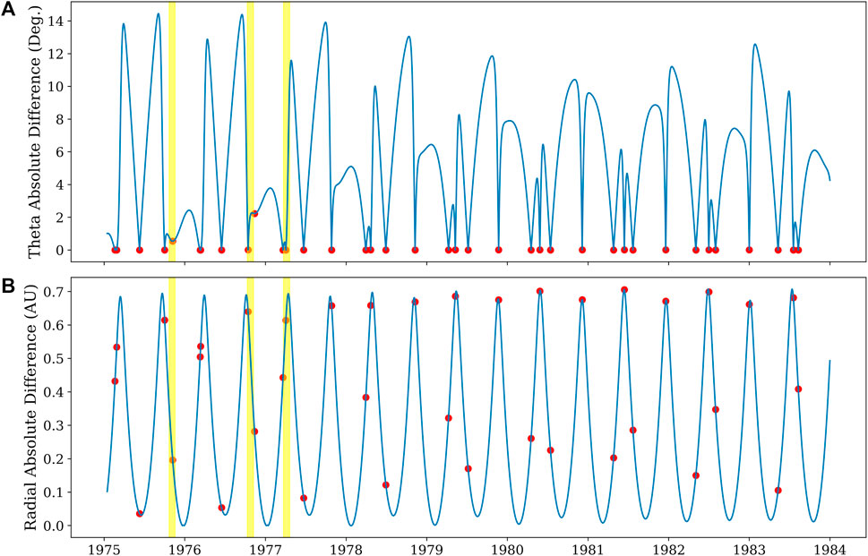
FIGURE 3. Latitude and radial absolute difference between Helios 1 and Earth Trajectories. The red dots represent the local minima for latitude absolute difference between Helios 1 and Earth.

For our first comparison, we focus on CR 1634, which occurred between 10/22/1 975 and 11/18/1 975. During this time, Helios 1 spanned from 136.14R_S to 187.08R_S, with a mean distance from the Sun of 165.67R_S. Thus, in terms of separation from Earth, it was, on average, closer to the Sun by 50R_S or 0.23 AU. Figure 4A summarizes the HUX mapping of smoothed Helios data (green/red/purple curves) with OMNI data at 1 AU. Each of the curves assumes that the Helios spacecraft is located at the minimum (green), mean (red) or maximum (purple) spacecraft distance during the interval, and, thus, provides a measure of the likely uncertainty in making this approximation. In general, we infer that the mean distance appears to give the best match with the observations. Several other features are notable. First, the main high-speed stream ($>700$ km s⁻¹) at 180° matches well between the mapped and observed values, including some of the smaller scale structure within it. Second, given our confidence from the previous point, we suggest that where there are OMNI data gaps at $\sim 45-100°$ and $\sim 201-280°$, the mapped Helios 1 data perhaps provides a reasonable prediction for what would have been observed, in particular, a modest high-speed (600 km s⁻¹) stream and slow/steady solar wind, respectively.

FIGURE 4

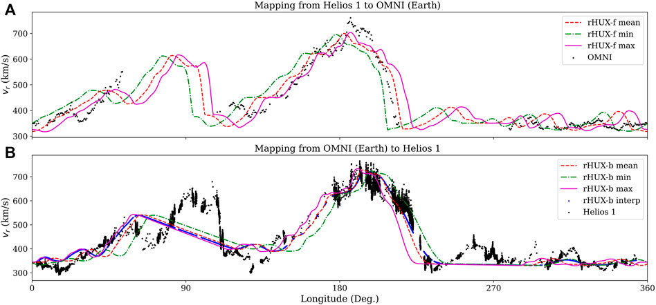
FIGURE 4. (A) Comparison of mapped solar wind streams from Helios 1 spacecraft with Earth-based measurements (OMNI) for CR 1634. The three coloured curves correspond to the minimum, mean, and maximum (green, red, and purple, respectively) of Helios 1 radial distance from the Sun for this period. (B) As (A) but mapping Earth-based measurements (OMNI) back the location of the Helios 1 spacecraft.

In Figure 4B, we compare OMNI data mapped back to the location of Helios 1 showing that the procedure works well in both directions. The missing data in the OMNI dataset are mapped back as straight, unstructured lines, centred at more westerly longitudes than at Earth; $\sim 90°$ and $\sim 270°$. Similar points can be made here, as for the outward mapping case. The main inference to be drawn, however, is that HUX-f and HUX-b are, at least on large scales performing well.

Next, we consider CR 1647, which occurred between 10/11/1 976 and 11/07/1 976. Unlike the previous case, here, there are no significant data gaps in the OMNI dataset, but one substantial gap in the Helios 1 data between $\sim 285°$ and $\sim 330°$ longitude (Figure 5). The minimum/mean/max separations were 69.5/102.4/140.3 R_S. Focusing first on the Helios 1 data mapped outward to the location of Earth, we note that the modest ($\sim 500$ km s⁻¹) stream centred at $\sim 80°$ is well captured by the Helios-mapped data, and the HUX-f min profile, in particular. This makes sense as the data at earlier longitudes corresponds to later times during the interval, which, as can be seen from Figure 3B, occurred during minimum radial separation (middle yellow box). The large high-speed stream centred at $\sim 300°$ is missing from the HUX-f mapped Helios data. However, this was also when a substantial gap in Helios 1 data occurred. Finally, it is worth noting here, albeit unsurprisingly, that intervals of slow and steady solar wind are mapped correctly from one spacecraft to the other (e.g., $\sim 135°-270°$).

FIGURE 5

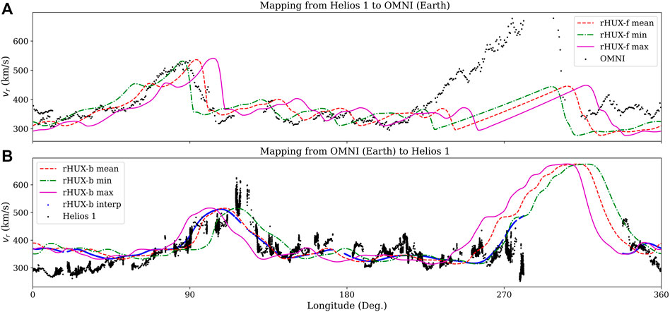
FIGURE 5. As Figure 4, but for CR1647.

As a final illustration of mapping between Helios 1 and Earth, in Figure 6, we compare outwardly-mapped Helios 1 data and inwardly mapped OMNI data for CR 1953. Again, there are relatively few missing data points at Earth, but a large gap in Helios 1 data in the range: $\sim -15°\to 90°$. Overall, the comparisons hold up well. In this case, the fact that the missing Helios 1 data occurred during an interval where the observed speed at Earth was slow and constant, led to a reasonable mapping throughout. It is also worth noting for this rotation, that the sub-structure within the main high-speed stream centered around $\sim 180°$ appears to have been captured by the HUX-mapped data; in particular, three distinct sub-streams. However, while the amplitude of these sub-streams is reproduced well at 1 AU, they are more attenuated at Helios 1. In fact, comparing the observed peaks of these streams, we note that they reached almost $\sim 800$ km s⁻¹ at Helios 1, but did not even reach $\sim 700$ km s⁻¹ at Earth.

FIGURE 6

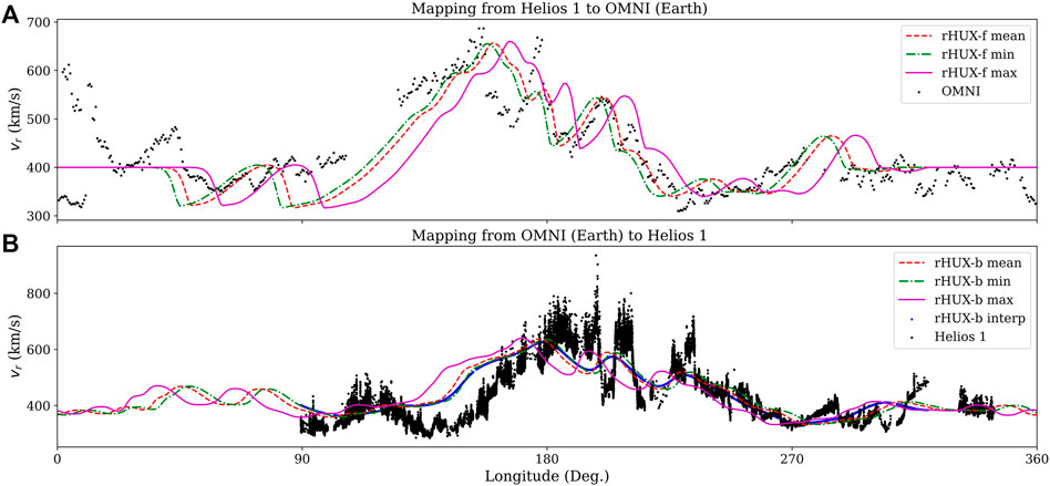
FIGURE 6. As Figure 4, but for CR1653.

4.2 Mapping From Helios 2 to OMNI and OMNI to Helios 2

During the almost four-year interval during which Helios 2 returned results, there were almost 20 points where the latitude difference between it and Earth vanished (Figure 7A). Of these, approximately half occurred with a radial separation of more than 0.3 AU (Figure 7B). We again identified three specific Carrington rotations to illustrate several key points: CR 1653, 1667, and 1675 (yellow shaded intervals). The first interval coincided with the last interval analyzed for Helios 1, and the remaining two were separated by approximately 1 year from one another. Thus, they represent solar minimum, and early ascending phases of the solar activity cycle.

FIGURE 7

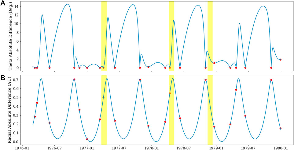
FIGURE 7. As Figure 3, but for Helios 2.

Figure 8 compares mapped Helios 2 data with OMNI data (a) and mapped OMNI data with Helios 2 (b) for 1653. In both cases, the comparisons demonstrate that the HUX-f and HUX-b techniques accurately extrapolate data from one location to another. Here, it is particularly noteworthy that the three major sub-streams around $\sim 180°$ are captured by each mapping; however, as before, while the amplitude of the streams matches well in the outward mapping to 1 AU, it is attenuated during the inward mapping to the location of Helios 2.

FIGURE 8

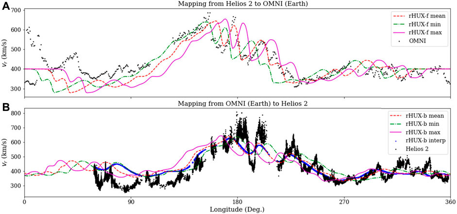
FIGURE 8. (A) Comparison of mapped solar wind streams from Helios 2 spacecraft with Earth-based measurements (OMNI) for CR 1653. The three coloured curves correspond to the minimum, mean, and maximum (green, red, and purple, respectively) Helio 2 radial distance from the Sun for this period. (B) As (A) but mapping Earth-based measurements (OMNI) back the location of the Helios 2 spacecraft.

Figure 9 provides a complementary illustration of the impact of missing data intervals. CR 1667 spanned the interval: 04/09/1 978–05/06/1 978. In this case, there were substantial data gaps at Earth ($\sim 85°-160°$) and Helios 2 ($\sim 0°-120°$). Again, where data and mapped results coincide, the large-scale comparisons are good: streams are reasonably well reproduced, both in terms of phase and amplitude. Additionally, given the good matches where data are available, the mapped data in the intervals of missing data, such as the high-speed stream centred at $\sim 75°$ in panel (b), can be given a reasonably high confidence of being present.

FIGURE 9

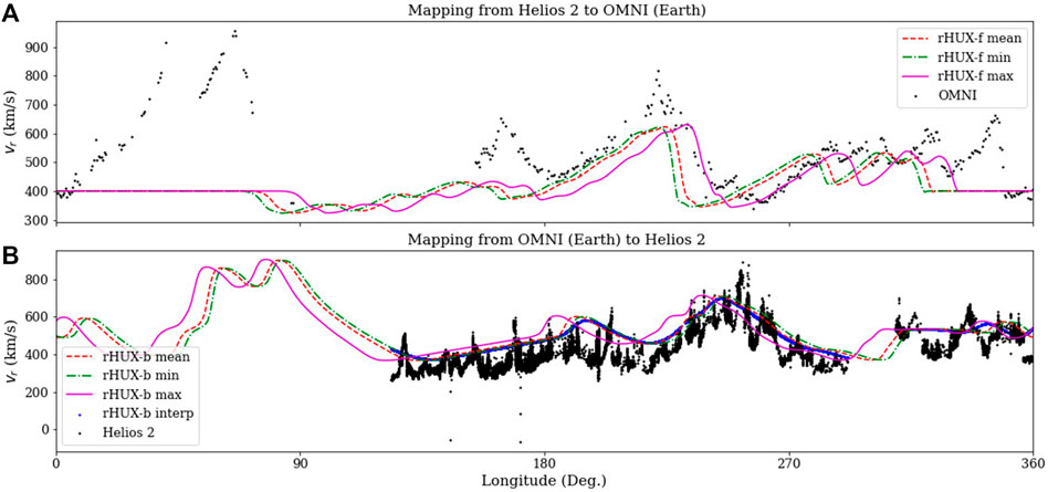
FIGURE 9. As Figure 8, but for CR1667.

As a final illustration, in Figure 10 we compare data and mapped profiles for CR 1675, which occurred during the interval from 11/13/1 978 to 12/10/1 978. Only one small data gap occurred in the Helios 2 dataset ($\sim 310°-360°$). While most of the stream structure is captured well with either the inward or outward mappings, there is a notable disagreement in the range $\sim 0°-30°$. This is not associated with any missing data, but likely reflects an underlying difference in the latitutinal separation of the spacecraft. Note that from Figure 7A, while the interval began with the two spacecraft being latitudinally-aligned, for much of the interval, they were separated by $\sim 1°-2°$. Of course, it is also possible that the divergence in structure is due to transient effects, or some combination thereof.

FIGURE 10

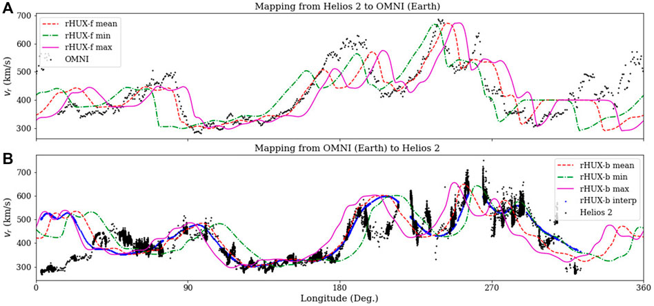
FIGURE 10. As Figure 8, but for CR1675.

5 Summary and Discussion

In this study, we have further refined a simple technique for mapping solar wind streams from one location to another location in the inner heliosphere. Additionally, we applied the technique to a variety of solar wind datasets, focusing on Helios 1 and 2 and near-Earth (OMNI), to illustrate some of the capabilities and limitations of such an approach. We suggest that rHUX can support studies aimed at understanding the evolution of solar wind streams from the Sun to 1 AU (and beyond) as well as inferring the likely source regions of observed solar wind plasma. Moreover, it can support real-time forecasts, by providing a computationally economical and efficient method for predicting stream structure at various locations in the heliosphere.

As noted in papers 1 and 2, the HUX technique relies on a number of potentially significant assumptions and approximations, including: (1) that all observed structure is quasi-stationary; (2) that non-radial propagation can be ignored; and (3) that the simplification of the momentum equation is reasonable (i.e., that several forces (e.g., gravity, magnetic and thermal pressure) can be neglected). In addition to these, we also assumed that the spacecraft did not significantly move in radial distance during the mapping interval (one solar rotation). As can be seen from the comparisons in Figures 4–6; Figures 8–10, this can introduce errors of up to $\sim 10°$.

Focusing specifically on our simplification of the momentum equation, we note that it has been previously shown that the ram (or dynamic) pressure of the solar wind at 1 AU near the ecliptic exceeds the thermal pressure by a factor of ∼ 200 (Feldman et al., 1977; Riley, 1999). Moreover, the plasma-β is typically $\sim 2$ (Wilson et al., 2018). Thus, the dynamic pressure substantially dominates over both the thermal and magnetic pressure terms. Additionally, the gravity term ceases to control the coronal plasma beyond a few solar radii, at which point the solar wind begins accelerating away from the Sun, and is certainly negligible by 20, − , 30R_S, where the present model is applied.

Our results are in apparent disagreement with those of Macneil et al. (Macneil et al., 2021), who found that by Nolte and Roelof (Nolte and Roelof, 1973), at least to some extent, errors introduced by neglecting solar wind acceleration and non-radial (azimuthal) flows tended to cancel. They concluded that the “constant speed radial solar wind backmapping” technique was likely as accurate and simpler to apply than more sophisticated approaches, including the various iterations of the HUX technique. While this is certainly possible, the results from the current study do not show any obvious longitudinal offsets. Of course, to firmly identify such an effect might require a more comprehensive study. More importantly, however, the constant speed backmapping technique does not address the evolution of solar wind streams, which was one of the main motivations for its development. Thus, if the objective is simply to identify the likely source regions of plasma observed in situ, the constant speed approximation might be sufficient; however, if knowledge of stream evolution is paramount, then the HUX technique should be used.

We treated the 3-D MHD model results as the “gold standard” or “ground truth”, and previous studies have shown that the MHD model is, in general, reasonably accurate [e.g., (Riley et al., 2001; Riley et al., 2011; Riley et al., 2021)]. Yet, despite this, it is important to note that the MHD model solutions can exhibit numerical dissipation effects that are not physically apparent. Thus, it should be borne in mind that a small contribution to the error in the HUX technique may be spurious; however, since we have no independent way to evaluate this (such as though an analytic solution), this remains speculation. In any case, this is likely to be a relatively small effect.

Our investigation has focused on intervals surrounding solar minimum, for which transient activity is expected to be minimal. However, the HUX approach has also been refined to explicitly allow for temporal variations, including large-scale CMEs (Owens et al., 2020). One interesting forecasting application would be to use the results produced from HUX as the ambient solar wind into which CMEs are launched. Indeed, a promising “proof of concept” has already been demonstrated by Barnard et al. (Barnard et al., 2020) using heliographic imager data. More generally, however, a range of ICME models could be launched into the HUX-derived 3-D background solar wind. We anticipate that the relatively high accuracy of the ambient solar wind produced by rHUX would lead to better estimates of CME shock arrival times at multiple locations in the heliosphere (Wold et al., 2018; Verbeke et al., 2019). Moreover, given the simplicity of the approach it would be straightforward to develop a large set of realizations as well as to explore the sensitivity of the parameter phase space. By developing hindcasts of the shock arrival times at NASA’s CCMC CME Scoreboard database (Riley et al., 2018), it should be possible to optimize the algorithm to produce at least modestly more accurate predictions.

Data Availability Statement

The model results used in this study can be found in the HUX repository, located at https://github.com/predsci/HUX-paper3. This research made use of HelioPy, a community-developed Python package for space physics \citep[]{heliopy21} to obtain data from NASA's Space Physics Data Facility (SPDF) website (https://cdaweb.gsfc.nasa.gov/index.html/), along with PsiPy to download PSI's MAS (Magnetohydrodynamics Algorithm outside a Sphere) model results \citep[]{psipy}.

Author Contributions

PR and OI developed the theoretical formalism for the ideas presented here. OI wrote the Python code to test the concepts with minor contributions from PR. PR and OI jointly wrote the paper.

Funding

The authors gratefully acknowledge support from NASA (80NSSC18K0100, NNX16AG86G, 80NSSC18K1129, 80NSSC18K0101, 80NSSC20K1285, 80NSSC18K1201, and NNN06AA01C), NOAA (NA18NWS4680081), and the U.S. Air Force (FA9550-15-C-0001).

Conflict of Interest

Authors OI and PR were employed by the company Predictive Science Inc.

Publisher’s Note

All claims expressed in this article are solely those of the authors and do not necessarily represent those of their affiliated organizations, or those of the publisher, the editors and the reviewers. Any product that may be evaluated in this article, or claim that may be made by its manufacturer, is not guaranteed or endorsed by the publisher.

Supplementary Material

The Supplementary Material for this article can be found online at: https://www.frontiersin.org/articles/10.3389/fspas.2021.795323/full#supplementary-material

Footnotes

¹In paper 2, this condition was mistakenly written with the fraction inverted; however, in the code that was distributed with the publication, it was implemented correctly.

References

Barnard, L., Owens, M. J., Scott, C. J., and de Koning, C. A. (2020). Ensemble Cme Modeling Constrained by Heliospheric Imager Observations. AGU Adv. 1, e2020AV000214. doi:10.1029/2020av000214

CrossRef Full Text | Google Scholar

Courant, R., Friedrichs, K., and Lewy, H. (1967). On the Partial Difference Equations of Mathematical Physics. IBM J. Res. Dev. 11, 215–234. doi:10.1147/rd.112.0215

CrossRef Full Text | Google Scholar

Feldman, W., Asbridge, J., Bame, S., and Gosling, J. (1977). "Plasma and Magnetic Fields From the Sun," in The Solar Output and its Variation. Editor O. R. White (Boulder: Col. Assoc. Univ. Press), 351–382.

Google Scholar

Finley, A. J., Matt, S. P., Réville, V., Pinto, R. F., Owens, M., Kasper, J. C., et al. (2020). The Solar Wind Angular Momentum Flux as Observed by Parker Solar Probe. Astrophysical J. 902, L4. doi:10.3847/2041-8213/abb9a5

CrossRef Full Text | Google Scholar

Gosling, J. T., and Pizzo, V. J. (1999). Formation and Evolution of Corotating Interaction Regions and Their Three Dimensional Structure. Corotating interaction regions. 89, 21–52. doi:10.1007/978-94-017-1179-1_3

CrossRef Full Text | Google Scholar

King, J., and Papitashvili, N. (2005). Solar Wind Spatial Scales in and Comparisons of Hourly Wind and Ace Plasma and Magnetic Field Data. J. Geophys. Res. Space Phys. 110, 1–8. doi:10.1029/2004ja010649

CrossRef Full Text | Google Scholar

Kivelson, M. G., and Russell, C. T. (1995). Introduction to Space Physics. Cambridge: Cambridge University Press.

Google Scholar

LeVeque, R. J. (1992). Numerical Methods for Conservation Laws. Basel, Switzerland: Lectures in mathematics Birkhäuser.

Google Scholar

LeVeque, R. J. (2002). Finite Volume Methods for Hyperbolic Problems. Cambridge Texts in Applied Mathematics. Cambridge: Cambridge University Press.

Google Scholar

MacCormack, R. (1969). The Effects of Viscosity in Hypervelocity Impact Cratering. AIAA. 69, 354. doi:10.2514/2.6901

CrossRef Full Text | Google Scholar

Macneil, A. R., Owens, M. J., Finley, A. J., and Matt, S. P. (2021). A Statistical Evaluation of Ballistic Backmapping for the Slow Solar Wind: The Interplay of Solar Wind Acceleration and Corotation. Monthly Notices R. Astronomical Soc. 509, 2390–2403. doi:10.1093/mnras/stab2965

CrossRef Full Text | Google Scholar

Mariani, F., Villante, U., Bruno, R., Bavassano, B., and Ness, N. F. (1979). An Extended Investigation of Helios 1 and 2 Observations: the Interplanetary Magnetic Field Between 0.3 and 1 AU. Sol. Phys. 63, 411–421. doi:10.1007/BF00174545

CrossRef Full Text | Google Scholar

Neugebauer, M., and Snyder, C. W. (1966). Mariner 2 Observations of the Solar Wind: 1. Average Properties. J. Geophys. Res. 71, 4469–4484. doi:10.1029/jz071i019p04469

CrossRef Full Text | Google Scholar

Nolte, J., and Roelof, E. (1973). Large-Scale Structure of the Interplanetary Medium. Solar Phys. 33, 483–504. doi:10.1007/BF00152395

CrossRef Full Text | Google Scholar

Owens, M., Lang, M., Barnard, L., Riley, P., Ben-Nun, M., Scott, C. J., et al. (2020). A Computationally Efficient, Time-Dependent Model of the Solar Wind for Use as a Surrogate to Three-Dimensional Numerical Magnetohydrodynamic Simulations. Solar Phys. 295, 1–17. doi:10.1007/s11207-020-01605-3

CrossRef Full Text | Google Scholar

Pizzo, V. (1978). A Three-Dimensional Model of Corotating Streams in the Solar Wind, 1. Theoretical Foundations. J. Geophys. Res. 83, 5563–5572. doi:10.1029/ja083ia12p05563

CrossRef Full Text | Google Scholar

Pizzo, V. J., and Gosling, J. T. (1994). 3-d Simulation of High-Latitude Interaction Regions: Comparison With Ulysses Results. Geophys. Res. Lett. 21, 2063–2066. doi:10.1029/94gl01581

CrossRef Full Text | Google Scholar

Poedts, S., Lani, A., Scolini, C., Verbeke, C., Wijsen, N., Lapenta, G., et al. (2020). European Heliospheric Forecasting Information Asset 2.0. J. Space Weather Space Clim. 10, 57. doi:10.1051/swsc/2020055

CrossRef Full Text | Google Scholar

Poirier, N., Kouloumvakos, A., Rouillard, A. P., Pinto, R. F., Vourlidas, A., Stenborg, G., et al. (2020). Detailed Imaging of Coronal Rays with the parker Solar Probe. Astrophysical J. Suppl. Ser. 246, 60. doi:10.3847/1538-4365/ab6324

CrossRef Full Text | Google Scholar

Priest, E., and Forbes, T. (2000). Magnetic Reconnection: MHD Theory and Applications. Cambridge: Cambridge University Press.

Google Scholar

Réville, V., Velli, M., Panasenco, O., Tenerani, A., Shi, C., Badman, S. T., et al. (2020). The Role of Alfvén Wave Dynamics on the Large-Scale Properties of the Solar Wind: Comparing an mhd Simulation With Parker Solar probe e1 Data. Astrophysical J. Suppl. Ser. 246, 24. doi:10.3847/1538-4365/ab4fef

CrossRef Full Text | Google Scholar

Riley, P. (1999). Cme Dynamics in a Structured Solar Wind. AIP Conf. Proc. (American Inst. Physics). 471, 131–136. doi:10.1063/1.58741

CrossRef Full Text | Google Scholar

Riley, P. (2021). Psipy. version 0.0.1. Les Ulis, France: EDP Sciences for European Southern Observatory. doi:10.5281/zenodo.5055879

CrossRef Full Text | Google Scholar

Riley, P., Downs, C., Linker, J. A., Mikic, Z., Lionello, R., and Caplan, R. M. (2019). Predicting the Structure of the Solar Corona and Inner Heliosphere during Parker Solar Probe 's First Perihelion Pass. Astrophysical J. 874, L15. doi:10.3847/2041-8213/ab0ec3

CrossRef Full Text | Google Scholar

Riley, P., and Gosling, J. T. (1998). Do coronal Mass Ejections Implode in the Solar Wind? Geophys. Res. Lett. 25, 1529–1532. doi:10.1029/98gl01057

CrossRef Full Text | Google Scholar

Riley, P., and Issan, O. (2021). Using a Heliospheric Upwinding Extrapolation Technique to Magnetically Connect Different Regions of the Heliosphere. Front. Phys. 9, 268. doi:10.3389/fphy.2021.679497

CrossRef Full Text | Google Scholar

Riley, P., Linker, J. A., Lionello, R., and Mikic, Z. (2012). Corotating Interaction Regions During the Recent Solar Minimum: The Power and Limitations of Global Mhd Modeling. J. Atmos. Solar-Terrestrial Phys. 83, 1–10. doi:10.1016/j.jastp.2011.12.013

CrossRef Full Text | Google Scholar

Riley, P., Linker, J. A., and Mikić, Z. (2001). An Empirically-Driven Global MHD Model of the Solar Corona and Inner Heliosphere. J. Geophys. Res. 106, 15889–15901. doi:10.1029/2000JA000121

CrossRef Full Text | Google Scholar

Riley, P., Lionello, R., Caplan, R. M., Downs, C., Linker, J. A., Badman, S. T., et al. (2021). Using Parker Solar Probe Observations During the First Four Perihelia to Constrain Global Magnetohydrodynamic Models. Astron. Astrophysics. 650, A19. doi:10.1051/0004-6361/202039815

CrossRef Full Text | Google Scholar

Riley, P., Lionello, R., Linker, J. A., Mikic, Z., Luhmann, J., and Wijaya, J. (2011). Global MHD Modeling of the Solar Corona and Inner Heliosphere for the Whole Heliosphere Interval. Sol. Phys. 274, 361–377. doi:10.1007/s11207-010-9698-x

CrossRef Full Text | Google Scholar

Riley, P., and Lionello, R. (2011). Mapping Solar Wind streams From the sun to 1 au: A comparison of techniques. Sol. Phys. 270, 575–592. doi:10.1007/s11207-011-9766-x

CrossRef Full Text | Google Scholar

Riley, P., Mays, M. L., Andries, J., Amerstorfer, T., Biesecker, D., Delouille, V., et al. (2018). Forecasting the Arrival Time of Coronal Mass Ejections: Analysis of the Ccmc Cme Scoreboard. Space Weather. 16, 1245–1260. doi:10.1029/2018sw001962

CrossRef Full Text | Google Scholar

Rosenbauer, H., Schwenn, R., Marsch, E., Meyer, B., Miggenrieder, H., Montgomery, M. D., et al. (1977). A Survey on Initial Results of the HELIOS Plasma Experiment. J. Geophys. Z. Geophys. 42, 561–580.

Google Scholar

Schwenn, R., and Marsch, E. (1990). Physics of the Inner Heliosphere. 1. Large-Scale Phenomena. Phys. Chem. Space. 20, 1–282.

CrossRef Full Text | Google Scholar

Shiota, D., Kataoka, R., Miyoshi, Y., Hara, T., Tao, C., Masunaga, K., et al. (2014). Inner Heliosphere Mhd Modeling System Applicable to Space Weather Forecasting for the Other Planets. Space Weather. 12, 187–204. doi:10.1002/2013sw000989

CrossRef Full Text | Google Scholar

Stansby, D., Rai, Y., Argall, M., Jeffrey, B., Haythornthwaite, R., Erwin, N., et al. (2021). Heliopython/Heliopy: Heliopy 0.15.3. Zenodo. 15, 3. doi:10.5281/zenodo.4643882

CrossRef Full Text | Google Scholar

Van Leer, B. (1974). Towards the Ultimate Conservative Difference Scheme. Ii. Monotonicity and Conservation Combined in a Second-Order Scheme. J. Comput. Phys. 14, 361–370. doi:10.1016/0021-9991(74)90019-9

CrossRef Full Text | Google Scholar

Van Leer, B. (1977). Towards the Ultimate Conservative Difference Scheme. Iv. A New Approach to Numerical Convection. J. Comput. Phys. 23, 276–299. doi:10.1016/0021-9991(77)90095-X

CrossRef Full Text | Google Scholar

Verbeke, C., Mays, M. L., Temmer, M., Bingham, S., Steenburgh, R., Dumbović, M., et al. (2019). Benchmarking Cme Arrival Time and Impact: Progress on Metadata, Metrics, and Events. Space Weather. 17, 6–26. doi:10.1029/2018sw002046

CrossRef Full Text | Google Scholar

Wilson, L. B., Stevens, M. L., Kasper, J. C., Klein, K. G., Maruca, B. A., Bale, S. D., et al. (2018). The Statistical Properties of Solar Wind Temperature Parameters Near 1 au. Astrophysical J. Suppl. Ser. 236, 41. doi:10.3847/1538-4365/aab71c

CrossRef Full Text | Google Scholar

Wold, A. M., Mays, M. L., Taktakishvili, A., Jian, L. K., Odstrcil, D., and MacNeice, P. (2018). Verification of Real-Time WSA−ENLIL+Cone Simulations of CME Arrival-Time at the CCMC From 2010 to 2016. J. Space Weather Space Clim. 8, A17. doi:10.1051/swsc/2018005

CrossRef Full Text | Google Scholar