Precursor identification for strong flares based on anomaly detection algorithm

1 Introduction

A solar flare is one of the major eruptive phenomena that occur in the solar atmosphere (Kahler, 1992). It is often accompanied with solar energetic particle acceleration (Reames, 1999) and coronal mass ejections [CMEs (Chen, 2011; Webb and Howard, 2012)] erupting into interplanetary space and sometimes, impacting the Earth and our technology, navigation, and communication systems (Gosling et al., 1991; Low, 1996; Wang and Zhang, 2007). Intense solar flares might lead to several kinds of geo-effectiveness, for example, ground level enhancement [GLE (Gopalswamy et al., 2012)] and sudden ionospheric disturbances [SIDs (Deshpande et al., 1972; Liu et al., 2004; Nie et al., 2022)].

There are many research studies based on observations and theoretical models of solar eruptions, focusing on the pre-eruption structures, triggering mechanisms, and the precursors indicating the potential eruption (Zirin and Liggett, 1987; Schrijver, 2009; Schrijver et al., 2011; Zhang et al., 2012; Kusano et al., 2020). It is widely accepted that solar flares are related to reconnection of topologically complex magnetic fields (Titov and Démoulin, 1999). The occurrence of solar flares is usually sensitive to some magnetic configuration of active regions (ARs), such as the polarity inversion lines, twisted flux tubes, and sheared loops. These magnetic structures of ARs and their statistical properties play an important role in discriminating the flaring and flare-quiet ARs (Barnes and Leka, 2006).

Developing solar flare prediction is one of the essential methods to prevent possible storm-like geo-effectiveness. One of the most widely used databases by the community is Space-Weather HMI Active Region Patches [SHARPs; (Bobra et al., 2014)]. It consists of the vector magnetic field images and many magnetic properties of ARs, such as the total unsigned flux (USFLU), the mean shear angle (MEANSHR), and the mean angle of field from radial (MEANGAM).

Many research studies have investigated the dataset and then developed and applied solar flare prediction models on them. In recent years, machine-learning algorithms have been applied in many research studies and made progress (Huang et al., 2018; Camporeale, 2019; Bhattacharjee et al., 2020; Krista and Chih, 2021; Nishizuka et al., 2021; Li et al., 2022). One of the most important achievements is the extraction of predictive features for flare classification. For example, Ahmed et al. (2013) applied machine-learning algorithms to extract and select the features highly related to solar flare prediction. Wang et al. (2019) applied the polarity inversion line (PIL) gradient masks and found that they have the potential to improve flare prediction. Then, Wang et al. (2020) extracted the features representing these PIL gradient masks by a machine-learning algorithm for strong-flare prediction. Sun et al. (2021) extracted both the spatial and topological features from SHARP patches and implied that using a single magnetic field component (radial magnetic field) can also derive strongly predictive features for flare classification. These studies were mainly focused on forecasting solar flares in 24-h in advance.

Moreover, considering the need for solar flare forecast in the operational application at space weather prediction centers, there is more work to do, especially in increasing the prediction accuracy and enlarging the prediction window (time-in-advance of solar flares), that is, it is important to develop an available model that can provide quantitative time-in-advance with promising evaluation metrics (i.e., prediction accuracy).

In this study, we assume that the magnetic configuration of active regions in quiet periods has certain similarities and can be considered “normal.” On the other hand, there should be some kinds of magnetic configuration of ARs that are related to strong flares. These magnetic features of ARs can be considered the precursor of strong flares and defined as “anomaly” compared to “normal.” We focus on two questions: first, whether these “anomaly” features can be detected and used to predict strong flares. Second, when these “anomaly” features occur, and whether they can be used to enlarge the prediction window and thus provide a quantitative time-in-advance in solar flare prediction.

Here, we introduce the data and methodology in Section 2 and then demonstrated a strong-flare classification model based on an anomaly detection algorithm and conduct result analysis in Section 3. The conclusion and discussion are presented in Section 4.

2 Data and methodology

2.1 Data preparation

According to the flare list from the National Oceanic and Atmospheric Administration (NOAA), we first divide the ARs into two categories: strong-flare ARs (which should be related to at least one strong flare) and non-strong-flare ARs. Strong flares are defined as M-class flares and above. Non-strong-flare ARs consist of both the ARs that produced no flares and the ARs that produced C-class flares and below.

To investigate the magnetic features of ARs, we used the radial magnetic field of SHARP patches in CEA coordinates (hmi.sharp_cea_720s) from 2010 to 2019. To avoid the projection effect, only those SHARP patches with centers located within 60° from the solar central meridian have been used in this study. We divided the datasets of SHARP patches into three groups as follows:

(1) Group train: it contains SHARP patches of the non-strong-flare ARs from 2010 to 2014. This group is used for model training. In this group, there are 845 non-strong-flare events.

(2) Group test normal: it contains SHARP patches of the non-strong-flare ARs from 2015 to 2019. This group is used for model testing on the non-strong-flare ARs. Thus, for the ARs that produced B-class flares and below, only one patch is selected randomly from each of the ARs and treated as a non-strong-flare event, while for the ARs that produced C-class flares, only the independent C-class flares are selected and treated as non-strong-flare events. Here, an independent C-class flare should meet the criteria that it is the only C-class flare in 4 days. In this group, there are 304 non-strong-flare events.

(3) Group test anomaly: it contains SHARP patches of the strong-flare ARs from 2010 to 2019. This group is used for model testing on the strong-flare ARs. Thus, only the independent M- and above class flares are selected and treated as strong-flare events. Here, an independent strong flare should meet the criteria that it is the only M- and above flare in 4 days. In this group, there are 107 strong-flare events.

It should be noted that the three groups (group train, group test normal, and group test anomaly) are independent. The data of each AR are assigned to one of the three groups. Moreover, for group test (including group test normal and group test anomaly), we only select the SHARP patches within the 3-day prediction window before the non-strong-flare events and the strong-flare events for model evaluation.

According the flow chart shown in Figure 1A, to obtain uniform and standard datasets that can be applied by machine-learning algorithms, we first randomly cut the SHARP patches into several square slices (with a size of 320 × 320 pixels). Then, we compressed the slices into smaller ones (with a size of 32 × 32 pixels) for fast computation purpose. Finally, we obtained datasets consisting of uniform and standard gray pictures (with a value in the range of 0–255). In this study, for each patch of strong-flaring ARs, which usually have a larger size than that of the square slices, we cut 10 slices randomly, while for each patch of those non-strong-flaring ARs, which usually is not obviously larger than the square slices, we cut no more than five slices randomly. Finally, we obtained 31,372 pictures for group train, 11,467 pictures for group test normal, and 58,099 pictures for group test anomaly.

FIGURE 1

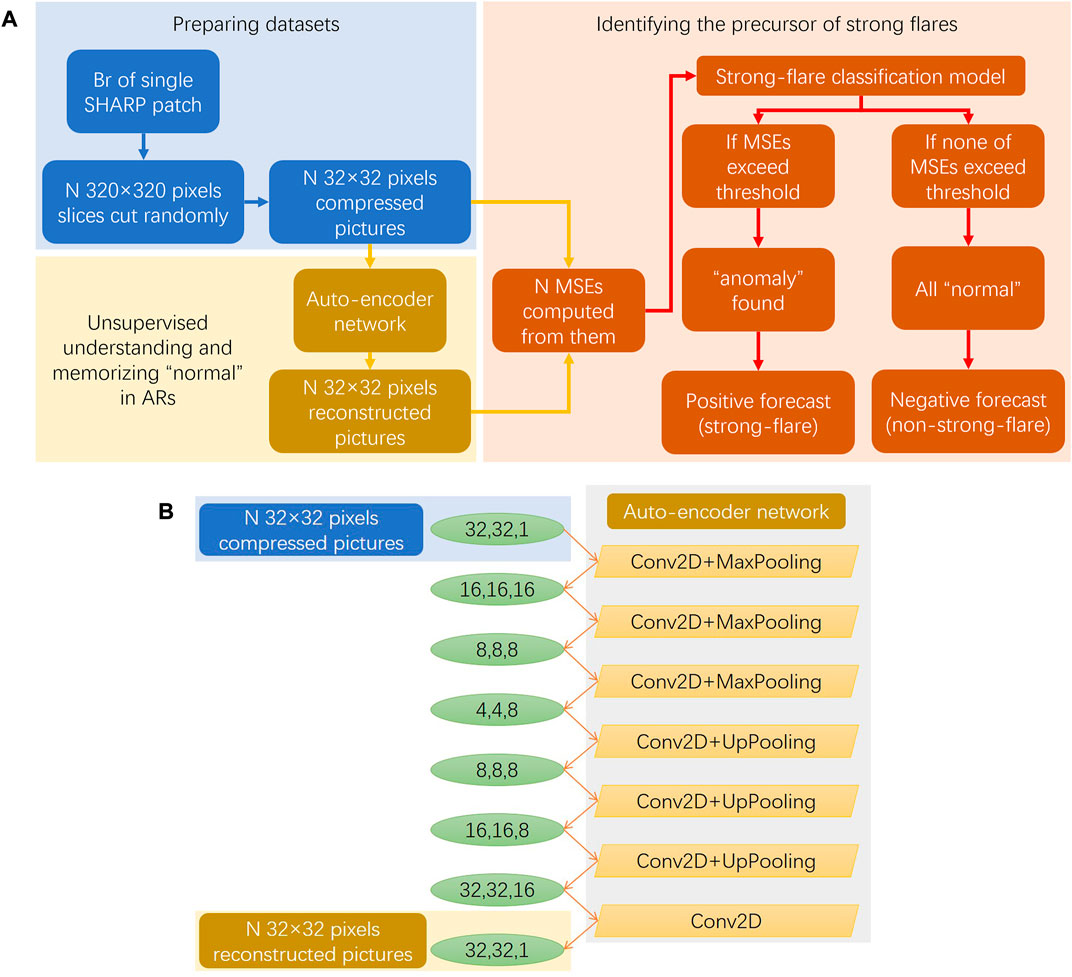
FIGURE 1. Flow chart for data preparation and model development. (A) is the flow chart. (B) illustrates the structure of the auto-encoder network.

We consider AR11158, for example, an X2.2 flare that erupted at 01:56 UTC, on 15 Feb 2011. The radial magnetic field of the SHARP patch corresponding to the onset of the flare is shown in Figure 2A. There are ten slices (with a size of 320 × 320 pixels) cut randomly from the patch. The locations of these slices are shown by colorful squares in Figure 2A. The final small slices (with a size of 32 × 32 pixels) compressed from the original slices are shown in the first and third rows in Figure 2B.

FIGURE 2

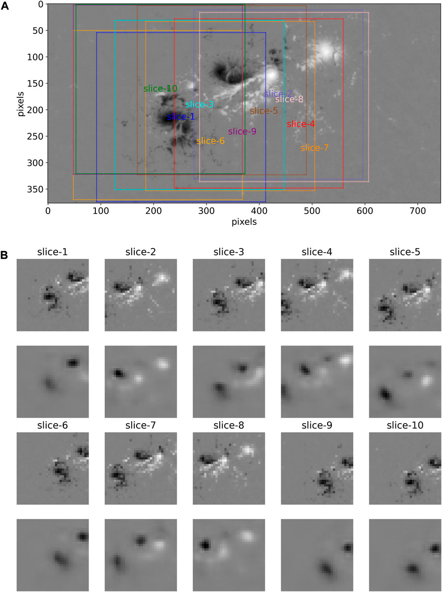
FIGURE 2. Illustration of the data preparation and the results by the auto-encoder network. (A) is the radial magnetic field of AR11158 (corresponding to SHARP patch number 377) before the X2.2 flare erupted at 01:56 UTC, on 15 Feb 2011. There are ten slices (with a size of 320 × 320 pixels) cut randomly from the original observations. (B) are the ten compressed slices in the first and third rows (with a size of 32 × 32 pixels, according to the ten slices in Figure 2A) and the corresponding reconstructed slices in the second and fourth rows derived by the auto-encoder network.

Another example is AR11192, an X1.6 flare that erupted at 14:28 UTC, on 22 Oct 2014. Similar to Figure 2, we illustrate the original radial magnetic field of the SHARP patch corresponding to the onset of the flare and the ten slices from it in Figure 3A, as well as the final compressed small slices in Fig 3b.

FIGURE 3

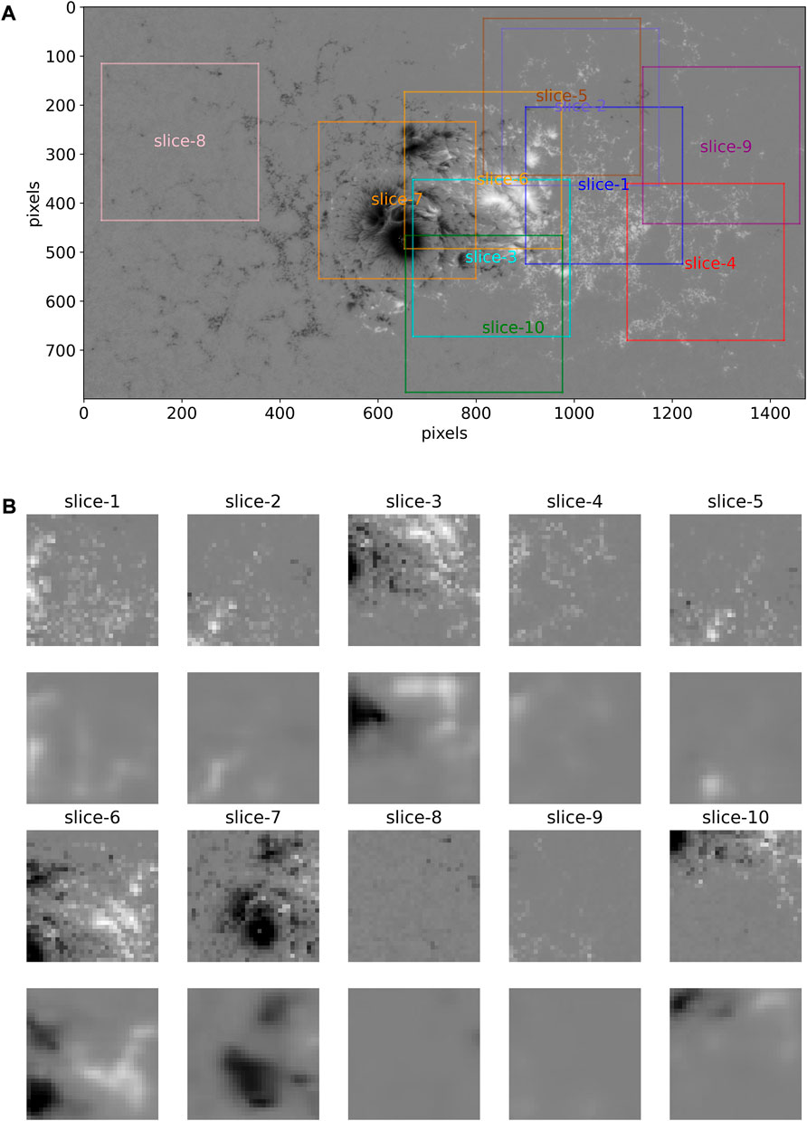
FIGURE 3. Illustration of the data preparation and the results by the auto-encoder network, similar to Figure 2. (A) is the radial magnetic field of AR12192 (corresponding to SHARP patch number 4698) before the X1.6 flare erupted at 14:28 UTC, on 22 Oct 2014. There are ten slices (with a size of 320 × 320 pixels) cut randomly from the original observations. (B) is similar to Figure 3B.

Comparing Figure 2 and Figure 3, it can be observed that for a relatively small patch (for example, AR11158), the cut slice strategy might lead to larger overlapping areas for those slices, while for a relatively large patch (for example, AR11192), it might lead to several non-overlapping areas which may represent widely differing magnetic structures and physical features. For example, slices 4, 8, and 9 are far away from the center of the patch in Figure 3A and do not capture the key magnetic features of AR11192. Therefore, we suggest cutting more slices randomly for larger patches in applications.

2.2 Unsupervised network

We assume that in group train, there might be a certain similarity in the magnetic configuration of the non-strong-flare ARs. As shown in the flow chart in Figure 1A, we first developed an unsupervised network using group train, aiming to understand and memorize these “normal” magnetic features of the non-strong-flare ARs and then identify the “anomaly” magnetic features of the strong-flare ARs by an anomaly detection algorithm using group test.

In this study, we adopt the auto-encoder network using the Keras package (https://keras.io) consisting of two-dimensional convolution layers (Conv2D), max pooling layers (MaxPooling), and up pooling layers (UpPooling). This network is an unsupervised machine-learning algorithm that reconstructs its input and extracts low-dimensional features as a representation of its inputs. The structure of the auto-encoder network is illustrated in Figure 1B. As shown in the flow chart in Figure 1A, we take the original pictures (slices with a size of 32 × 32 pixels) in group train as the input and feed them into the auto-encoder network to obtain reconstructed pictures (slices with a size of 32 × 32 pixels). During the training process, the unsupervised network will understand and memorize the “normal” magnetic features of the non-strong-flare ARs. Moreover, after training, we can also feed the group test as an input into the network and obtain reconstructed pictures for further analysis.

Taking the two strong-flare ARs, AR11158 in Figure 2B and AR11192 in Figure 3B, for example, the ten slices (input of the auto-encoder network) are shown in the first and third rows and the reconstructed slices (output of the auto-encoder network) in the second and fourth rows accordingly. It can be observed that the reconstructed pictures are blurred due to the limitations of the auto-encoder network with a relatively simple structure. In some other pictures, the main features are well-captured. However, in some pictures, there are apparent differences between the original pictures and reconstructed pictures. It indicates that the network has not understood and memorized this type of magnetic features because they probably are not one of the typical features in the group train (consisting of the non-strong-flare ARs).

2.3 Anomaly detection algorithm

Anomaly detection is a widely used algorithm to detect the anomaly features or patterns that do not fit the normal features or patterns of a dataset. Here, to identify the “anomaly” that indicates the precursor of strong flares in ARs, it is essential to define the “normal” first. Based on the assumption that the auto-encoder network performs well in understanding and memorizing the “normal” magnetic features of non-strong-flare ARs, it can be inferred that

(1) the network has been trained in group train so that it should perform well in group train such that the reconstructed pictures should be similar to the original pictures, that is, the differences between the input and output in group train should be relatively small.

(2) The network should also perform well in group test normal, which consists of non-strong-flare ARs, that is, the differences between the input and output of the network in group test normal should also be as small as in group train.

(3) The network would not perform as well in the group test anomaly that consists of strong-flare ARs as in the other two groups, that is, the differences between some of the input and output of the network in group test anomaly (indicating “anomaly”) should be relatively large compared to those of group train and group test normal.

Here, we adopt the mean squared errors (MSEs) of the original pictures and reconstructed pictures derived by the auto-encoder network to quantitatively describe the differences between them. We computed and analyzed the MSEs using the group train, group test normal, and group test anomaly. The histograms of MSEs of the three groups are shown from the top to the bottom in Figure 4. It can be observed that Figure 4 is in accordance with the earlier mentioned points.

FIGURE 4

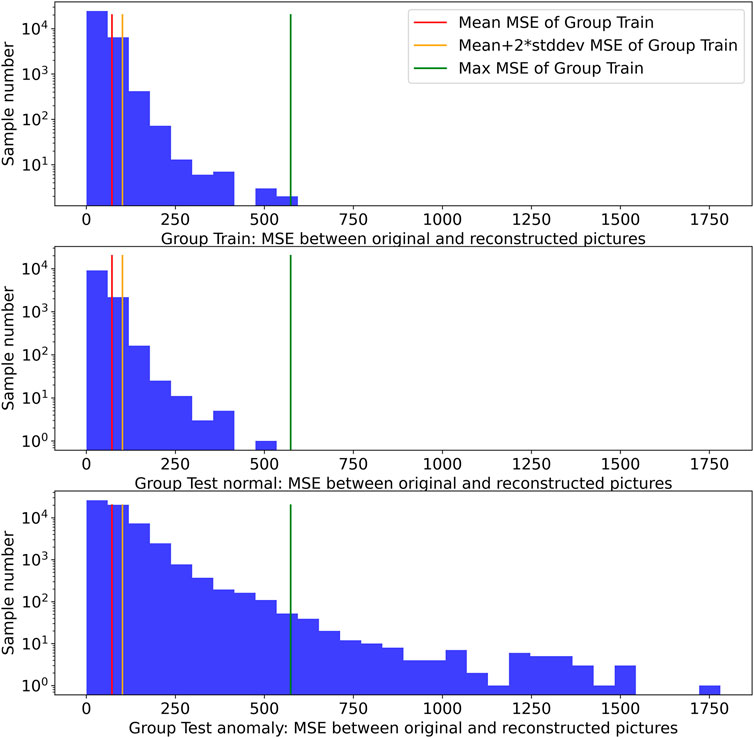
FIGURE 4. Histograms of MSEs of the original and reconstructed pictures derived by the auto-encoder network. From the top to the bottom, there is a histogram of MSEs calculated using group train, group test normal, and group test anomaly. The red, orange, and green vertical lines refer to the mean value, mean + 2 × standard deviation (std: dev), and maximum of MSEs using group train, respectively.

To identify when these “anomaly” features occur before strong flares, we investigate the MSEs of the pictures that belong to three different time windows before strong flares in group test anomaly and illustrate the histogram in Figure 5. The pictures in group test anomaly are divided into three subsets according to their time windows:

(1) Subset 1 contains pictures in the time range of (48h, 72h) before strong flares and is represented by a red histogram.

(2) Subset 2 contains pictures in the time range of (24h, 48h) before strong flares and is represented by an orange histogram.

(3) Subset 3 contains pictures taken no more than 24h before strong flares and is represented by a green histogram.

FIGURE 5

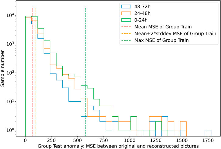
FIGURE 5. Histograms of MSEs of the original and reconstructed pictures in the group test anomaly derived by the auto-encoder network. The red, orange, and green histograms refer to the MSEs using subset 1 (pictures which are in the time range of (48h, 72h) before strong flares), subset 2 (pictures which are in the time range of (24h, 48h) before strong flares), and subset 3 (pictures which are no more than 24h before strong flares), respectively. Similar to the vertical lines in Figure 4, the red, orange, and green vertical dashed lines refer to the mean value, mean + 2 × standard deviation (std: dev), and maximum of MSEs using group train, respectively.

In Figure 5, the green dashed vertical line refers to the maximum MSE of group train. All pictures in group train have fewer MSEs by the reconstructed network, while it turns out that many pictures in group test anomaly have larger MSEs by the reconstructed network, which exceed the maximum MSE of group train. Even for some pictures which are of more than 1 day before the strong flares, their MSEs are also located on the right side of the green dashed line. It seems that the MSE of the original and reconstructed picture derived by the auto-encoder network is a good predictor to discriminate the pictures that indicate the magnetic “anomaly” of strong-flare ARs from other pictures that indicate the magnetic “normal” features of non-strong-flare ARs.

3 Model development and result analysis

3.1 Strong-flare classification model

As shown in the flow chart in Figure 1A, we developed a strong-flare classification model on the basis of identifying the precursor of strong flares using an anomaly detection algorithm. We choose the MSEs of the original pictures and reconstructed pictures derived by an auto-encoder network as a discrimination threshold for strong-flare forecasting.

For the strong-flare classification model, we carry out the following steps:

(1) For SHARP patches within the 3-day prediction window before the non-strong-flare events in group test normal, the ground truth should be classified as 0 (“normal,” “non-strong-flare”). For SHARP patches within the 3-day prediction window before the strong-flare events in group test anomaly, the ground truth should be classified as 1 (“anomaly,” “strong-flare”).

(2) Set a specific discrimination threshold, T_MSE.

(3) For N pictures (N is the number of the pictures and N equals 10 in this study) cut randomly from each SHARP patch in group test, we derive the corresponding reconstructed pictures by the auto-encoder network and compute N MSEs of them.

(4) If at least one in N MSEs from each SHARP patch exceeds the specific discrimination threshold (T_MSE), the forecast for the patch should be 1 (“anomaly,” “strong-flare”). Otherwise, the prediction should be 0 (“normal,” “non-strong-flare”).

3.2 Evaluation metrics

For a binary classification task like the strong-flare prediction, the confusion matrix is listed in Table 1. The true positive (TP) is the hit case where the strong-flare samples are correctly classified as the strong-flare category. The false positive (FP) is the false alarm case where the non-strong-flare samples are falsely classified as the strong-flare category. The false negative (FN) is the missing case where strong-flare samples are falsely classified as a non-strong-flare category. The true negative (TN) is the correct non-event case where non-strong-flare samples are correctly classified as the non-strong-flare category.

TABLE 1

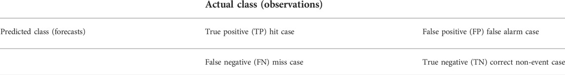
TABLE 1. Confusion matrix for binary classification.

Based on the confusion matrix, we adopt six evaluation metrics: accuracy, recall, precision, F1 score, ROC_AUC, and the first warning time-in advance for strong flares (FWT). The FWT is defined as the prediction time window for a strong flare. When our model sends the first warning (strong-flare forecast) for a strong-flare event, we calculate the time difference between the first warning time point and the start time of the strong-flare event according to the NOAA flare list and define it as the FWT. The average FWT is a good statistical parameter for model evaluation. The first four metrics are computed as follows:

$accuracy\left(o,p\right)=\frac{1}{N_{\mathit{samples}}}\sum _{i=0}^{N_{\mathit{samples}}}1\left(o_i=p_i\right),(1)$

$recall=\frac{TP}{TP+FN},(2)$

$precision=\frac{TP}{TP+FP},(3)$

$F1=\frac{2\times precision\times recall}{precision+recall}.(4)$

In addition, the receiver operating characteristic (ROC) curve illustrates the performance of a binary classification task as its discrimination threshold is varied. It is the fraction of the true positives out of the positives vs. the fraction of the false positives out of the negatives. The ROC_AUC computes the area under the ROC curve and summarizes it as one number.

For these first five metrics (accuracy, recall, precision, F1 score, and ROC_AUC), larger values indicate better discrimination ability of a binary classification model. The Scikit-learn package (https://scikit-learn.org) is used to calculate the abovementioned metrics. Moreover, a larger FWT indicates a longer time window before strong flares.

3.3 Model performance

To find the best strong-flare classification model, we need to find the best discrimination threshold of the MSEs. In Figure 6, the discrimination threshold is varying along the x-axis, and the six evaluation metrics (accuracy, recall, precision, F1 score, ROC_AUC, and FWT) for strong-flare classification are drawn accordingly. We find that the best classification model gives 94 hit cases (TP) and 13 miss cases (FN) from the group test anomaly (107 strong-flare cases) and 30 false alarm cases (FP) from the group test normal (304 strong-flare cases), thus providing the maximum F1 score of 0.8139. Also, the corresponding accuracy is 0.8954, the recall is 0.8785, the precision is 0.7581, the ROC_AUC is 0.8899, and the FWT is 45.24 h.

FIGURE 6

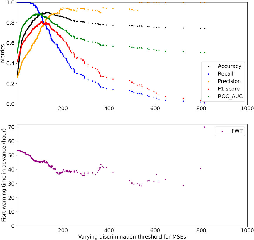
FIGURE 6. Evaluation metrics based on the group test with varying discrimination thresholds (set for MSEs of the original and reconstructed pictures). The accuracy, recall, precision, F1 score, ROC_AUC, and first warning time for strong flares in advance (FWT) are represented by the black, blue, orange, red, green, and purple points, respectively.

Taking AR11158 in Figure 2A and AR11192 in Figure 3A as examples, we first cut ten pictures randomly from them and draw them in Figure 2B and Figure 3B, respectively. Then, we applied the auto-encoder network to the ten small pictures and computed the MSEs between them and the corresponding reconstructed pictures. At last, we apply the best classification model to the MSEs, and it turns out that

(1) for all of the ten pictures in Figure 2B obtained from AR11158, their MSEs exceed the threshold, that is, there are “anomalies” as the precursor of strong flares found in these ten slices. Thus, we obtained a positive (strong-flare) forecast for AR11158 in Figure 2A.

(2) For the ten pictures in Figure 3B obtained from AR11129, the MSEs of the five pictures (slices 1, 3, 6, 7, and 10) exceed the threshold, that is, there are “anomalies” as the precursor of strong flares found in these five slices, while the MSEs of the other five pictures (slices 2, 4, 5, 8, and 9) are below the threshold. Thus, we obtained a positive (strong-flare) forecast for AR11192 in Figure 3A.

4 Conclusion and discussion

In this study, we assume that the magnetic configuration of ARs in quiet periods has certain similarities and can be considered “normal,” while there are some other magnetic features of ARs that are related to strong flares. They can be considered the precursor of strong flares and can be defined as “anomaly.” Our study aims to identify those “anomalies” and apply it in strong-flare forecasting.

Those similar features of non-strong-flare ARs can be understood and memorized by an unsupervised auto-encoder network. The SHARP dataset of non-strong-flare ARs in 2010–2014 has been used to train the auto-encoder network. We investigated the MSEs of the original pictures and reconstructed pictures derived by the auto-encoder and conducted a statistical analysis of the non-strong-flare samples. Then, we carried out the precursor identification for strong flares on the basis of an anomaly detection algorithm and developed a strong-flare classification model. Applying the classification model to the non-strong-flare AR samples in 2015–2019 and strong-flare AR samples in 2010–2019, we take the MSEs computed from the results by the auto-encoder network as a predictor and compare them with a specific threshold and finally obtained a strong-flare or non-strong-flare forecast for each sample.

We find that the “anomaly” magnetic features of ARs that indicate strong flares can be detected and used to predict strong flares. Also, we evaluate the performance of the classification model and obtain the quantitative time-in-advance for strong-flare prediction.

Our strong-flare classification model reaches an F1 score of 0.8139, an accuracy of 0.8954, a recall of 0.8785, a precision of 0.7581, and an ROC_AUC of 0.8899. Moreover, for those correctly predicted strong-flare events (94 M-class flares and above), our model reaches an average first warning time of 45.24 h. The results indicate that 1) the anomaly detection algorithm can help in both improving strong-flare prediction accuracy and enlarging the time in advance. 2) The precursor magnetic structures of ARs appear sometime before the strong-flare eruption, and thus the average maximum warning period for strong-flare prediction is close to 2 days. The results from our study about the application of the anomaly detection algorithm and the obtained average first warning time will be useful for future applications for space-weather solar flare prediction.

We noticed that the classification model falsely classify 13 strong-flare events into the non-strong-flare category. Moreover, 10 of them are M1 flare events. Two of them are M2 flare events; hence, these low-level strong flares are harder to predict than intense flares.

We also used the anomaly detection algorithm on another experiment based on the samples of group A (20 M5 class flares and above events) and group B (328 M4 class flares and below events). We trained a classification model based on independent group C (908 M4 class flares and below events). The model reaches an F1 score of 0.9626, an accuracy of 0.6501, a recall of 0.6842, a precision of 0.6667, and an ROC_AUC of 0.8159. The evaluation metrics of this experiment are relatively lower than those from the strong-flare classification model. It implies that there are obvious differences between the strong-flare ARs and non-strong-flare ARs.

We agree with Camporeale (2019) that embracing machine-learning into the space weather community is both a challenge and an opportunity. In the future, the application of machine-learning approaches in solar eruption prediction has the potential to help us develop models with better accuracy and longer prediction window to meet the needs of operational forecasting.

Data availability statement

The original contributions presented in the study are included in the article/Supplementary Material; further inquiries can be directed to the corresponding author.

Author contributions

JW, BL, and SL meet the authorship criteria and agree to be accountable for the content of the work.

Funding

JW was supported by the National Science Foundation of China (Grant No. 42074224), the Youth Innovation Promotion Association CAS (2021142), the Key Research Program of the Chinese Academy of Sciences (Grant No. ZDRE-KT-2021-3), and the Pandeng Program of National Space Science Center, Chinese Academy of Sciences.

Acknowledgments

We thank the SDO/HMI team members who contributed to the SDO mission. We wish to thank the anonymous referees for their valuable suggestions and comments that improved this work.

Conflict of interest

The authors declare that the research was conducted in the absence of any commercial or financial relationships that could be construed as a potential conflict of interest.

The handling editor declared a shared affiliation with the authors at the time of the review.

Publisher’s note

All claims expressed in this article are solely those of the authors and do not necessarily represent those of their affiliated organizations, or those of the publisher, the editors, and the reviewers. Any product that may be evaluated in this article, or claim that may be made by its manufacturer, is not guaranteed or endorsed by the publisher.

References

Ahmed, O. W., Qahwaji, R., Colak, T., Higgins, P. A., Gallagher, P. T., and Bloomfield, D. S. (2013). Solar flare prediction using advanced feature extraction, machine learning, and feature selection. Sol. Phys. 283, 157–175. doi:10.1007/s11207-011-9896-1

CrossRef Full Text | Google Scholar

Barnes, G., and Leka, K. D. (2006). Photospheric magnetic field properties of flaring versus flare-quiet active regions. iii. magnetic charge topology models. Astrophys. J. 646, 1303–1318. doi:10.1086/504960

CrossRef Full Text | Google Scholar

Bhattacharjee, S., Alshehhi, R., Dhuri, D. B., and Hanasoge, S. M. (2020). Supervised convolutional neural networks for classification of flaring and nonflaring active regions using line-of-sight magnetograms. Astrophys. J. 898, 98. doi:10.3847/1538-4357/ab9c29

CrossRef Full Text | Google Scholar

Bobra, M. G., Sun, X., Hoeksema, J. T., Turmon, M., Liu, Y., Hayashi, K., et al. (2014). The helioseismic and magnetic imager (hmi) vector magnetic field pipeline: Sharps–space-weather hmi active region patches. Sol. Phys. 289, 3549–3578. doi:10.1007/s11207-014-0529-3

CrossRef Full Text | Google Scholar

Camporeale, E. (2019). The challenge of machine learning in space weather: Nowcasting and forecasting. Space weather. 17, 1166–1207. doi:10.1029/2018SW002061

CrossRef Full Text | Google Scholar

Chen, P. F. (2011). Coronal mass ejections: Models and their observational basis. Living Rev. Sol. Phys. 8, 1. doi:10.12942/lrsp-2011-1

CrossRef Full Text | Google Scholar

Deshpande, S. D., Subrahmanyam, C. V., and Mitra, A. P. (1972). Ionospheric effects of solar flares - I. The statistical relationship between X-ray flares and SID’s. J. Atmos. Terr. Phys. 34, 211–227. doi:10.1016/0021-9169(72)90165-1

CrossRef Full Text | Google Scholar

Gopalswamy, N., Xie, H., Yashiro, S., Akiyama, S., Mäkelä, P., and Usoskin, I. G. (2012). Properties of ground level enhancement events and the associated solar eruptions during solar cycle 23. Space Sci. Rev. 171, 23–60. doi:10.1007/s11214-012-9890-4

CrossRef Full Text | Google Scholar

Gosling, J. T., McComas, D. J., Phillips, J. L., and Bame, S. J. (1991). Geomagnetic activity associated with Earth passage of interplanetary shock disturbances and coronal mass ejections. J. Geophys. Res. 96, 7831–7839. doi:10.1029/91JA00316

CrossRef Full Text | Google Scholar

Huang, X., Wang, H., Xu, L., Liu, J., Li, R., and Dai, X. (2018). Deep learning based solar flare forecasting model. I. Results for line-of-sight magnetograms. Astrophys. J. 856, 7. doi:10.3847/1538-4357/aaae00

CrossRef Full Text | Google Scholar

Kahler, S. W. (1992). Solar flares and coronal mass ejections. Annu. Rev. Astron. Astrophys. 30, 113–141. doi:10.1146/annurev.aa.30.090192.000553

CrossRef Full Text | Google Scholar

Krista, L. D., and Chih, M. (2021). A DEFT way to forecast solar flares. Astrophys. J. 922, 218. doi:10.3847/1538-4357/ac2840

CrossRef Full Text | Google Scholar

Kusano, K., Iju, T., Bamba, Y., and Inoue, S. (2020). A physics-based method that can predict imminent large solar flares. Science 369, 587–591. doi:10.1126/science.aaz2511

PubMed Abstract | CrossRef Full Text | Google Scholar

Li, M., Cui, Y., Luo, B., Ao, X., Liu, S., Wang, J., et al. (2022). Knowledge-informed deep neural networks for solar flare forecasting. Space weather. 20, e02985. doi:10.1029/2021SW002985

CrossRef Full Text | Google Scholar

Liu, J. Y., Lin, C. H., Tsai, H. F., and Liou, Y. A. (2004). Ionospheric solar flare effects monitored by the ground-based GPS receivers: Theory and observation. J. Geophys. Res. 109, A01307. doi:10.1029/2003JA009931

CrossRef Full Text | Google Scholar

Low, B. C. (1996). Solar activity and the corona. Sol. Phys. 167, 217–265. doi:10.1007/BF00146338

CrossRef Full Text | Google Scholar

Nie, W., Rovira-Garcia, A., Wang, Y., Zheng, D., Yan, L., and Xu, T. (2022). On the global kinematic positioning variations during the september 2017 solar flare events. JGR. Space Phys. 127, e30245. doi:10.1029/2021JA030245

CrossRef Full Text | Google Scholar

Nishizuka, N., Kubo, Y., Sugiura, K., Den, M., and Ishii, M. (2021). Operational solar flare prediction model using Deep Flare Net. Earth Planets Space 73, 64. doi:10.1186/s40623-021-01381-9

CrossRef Full Text | Google Scholar

Reames, D. V. (1999). Particle acceleration at the Sun and in the heliosphere. Space Sci. Rev. 90, 413–491. doi:10.1023/A:1005105831781

CrossRef Full Text | Google Scholar

Schrijver, C. J., Aulanier, G., Title, A. M., Pariat, E., and Delannée, C. (2011). The 2011 february 15 X2 flare, ribbons, coronal front, and mass ejection: Interpreting the three-dimensional views from the solar dynamics observatory and STEREO guided by magnetohydrodynamic flux-rope modeling. Astrophys. J. 738, 167. doi:10.1088/0004-637X/738/2/167

CrossRef Full Text | Google Scholar

Schrijver, C. J. (2009). Driving major solar flares and eruptions: A review. Adv. Space Res. 43, 739–755. doi:10.1016/j.asr.2008.11.004

CrossRef Full Text | Google Scholar

Sun, H., Manchester, W., and Chen, Y. (2021). Improved and interpretable solar flare predictions with spatial and topological features of the polarity inversion line masked magnetograms. Space weather. 19, e02837. doi:10.1029/2021SW002837

CrossRef Full Text | Google Scholar

Titov, V. S., and Démoulin, P. (1999). Basic topology of twisted magnetic configurations in solar flares. Astronomy Astrophysics 351, 707–720.

Google Scholar

Wang, J., Liu, S., Ao, X., Zhang, Y., Wang, T., and Liu, Y. (2019). Parameters derived from the SDO/HMI vector magnetic field data: Potential to improve machine-learning-based solar flare prediction models. Astrophys. J. 884, 175. doi:10.3847/1538-4357/ab441b

CrossRef Full Text | Google Scholar

Wang, J., Zhang, Y., Hess Webber, S. A., Liu, S., Meng, X., and Wang, T. (2020). Solar flare predictive features derived from polarity inversion line masks in active regions using an unsupervised machine learning algorithm. Astrophys. J. 892, 140. doi:10.3847/1538-4357/ab7b6c

CrossRef Full Text | Google Scholar

Wang, Y., and Zhang, J. (2007). A comparative study between eruptive X-class flares associated with coronal mass ejections and confined X-class flares. Astrophys. J. 665, 1428–1438. doi:10.1086/519765

CrossRef Full Text | Google Scholar

Webb, D. F., and Howard, T. A. (2012). Coronal mass ejections: Observations. Living Rev. Sol. Phys. 9, 3. doi:10.12942/lrsp-2012-3

CrossRef Full Text | Google Scholar

Zhang, J., Cheng, X., and Ding, M.-D. (2012). Observation of an evolving magnetic flux rope before and during a solar eruption. Nat. Commun. 3, 747. doi:10.1038/ncomms1753

PubMed Abstract | CrossRef Full Text | Google Scholar

Zirin, H., and Liggett, M. A. (1987). Delta spots and great flares. Sol. Phys. 113, 267–283. doi:10.1007/BF00147707

CrossRef Full Text | Google Scholar