Daedalus MASE (mission assessment through simulation exercise): A toolset for analysis of in situ missions and for processing global circulation model outputs in the lower thermosphere-ionosphere

1 Introduction

Daedalus MASE comprises a suite of modeling tools targeting processes related to ion-neutral interactions in the Lower Thermosphere and Ionosphere (LTI), a key interface region between Earth’s atmosphere and space. Within this region, the atmosphere transitions from being well-mixed and electrically neutral, to heterogeneous and partly ionized. Interactions between ions and neutrals maximize within the LTI, and in particular at altitudes from 100 to 200 km. These interactions lead to electrical currents, Pedersen and Hall conductivities and Joule or frictional heating, all of which maximize within this altitude range. Their approximation is a subject of extensive research, as these processes determine the energetics and dynamics within this region. Whereas the physics of these processes is well understood and is captured in Global Circulation Models (GCMs), their quantification is still largely unknown and shows large discrepancies between different models or even parameterizations within the same model. The reason is that their exact quantification requires the simultaneous and co-located measurement of an extensive list of many relevant parameters. Such comprehensive list of measurements includes ion, neutral and electron densities (N_i, N_n, N_e), ion and neutral composition (n_ix and n_nx), ion, electron and neutral temperatures (T_i, T_e and T_n), ion drifts v_i), neutral winds (u_n), electric field $(\vec{E})$, and magnetic field $(\vec{B})$; in the following these are termed primary observables or geophysical observables. Whereas some of the above geophysical observables can be provided via remote sensing, the combination of all parameters at the same location can only be achieved via in situ measurements from a fully instrumented satellite. This has never been achieved to date, as altitudes from 100 to 200 km constitute the least visited region of the near-Earth environment (Sarris. (2019); Palmroth et al. (2021)). This leads to large discrepancies between estimations of key parameters, such as Pedersen and Hall conductivities, electrical currents and energy inputs due to Joule heating, which, in turn, greatly affects our ability to model and predict, for example, neutral density enhancements, that are of key importance to satellite drag calculations.

Daedalus MASE was initially developed to assess the performance of the mission concept Daedalus: proposed to the European Space Agency’s Earth Explorer program (Sarris et al., 2020), Daedalus targets to perform in situ height-resolved measurements in the 100–200 km region from an eccentric low-perigee orbit. The main motivation for the Daedalus mission and its over-arching mission objective is to provide the first simultaneous and comprehensive set of in situ measurements of all physical quantities describing the lower thermosphere and ionosphere with the goal to explore and investigate the dominant processes that determine the energetics, dynamics, and chemistry of the region. Daedalus aims to make significant advancements and contributions to LTI physics/process understanding (e.g., Palmroth et al. (2021); Karlsson et al. (2020)), climatological specification/empirical models (e.g., Emmert et al. (2021)) and applications (e.g., Crisp et al. (2020)). One of the purposes of the development of Daedalus MASE was to demonstrate how the combination of all relevant primary observables enables the quantification of various products related to ion-neutral interaction processes. The purpose of Daedalus MASE was also to demonstrate that the mission requirements are sufficient to reach the Daedalus baseline mission objectives (ESA, 2020). This implies meeting performance metrics in terms of a) uncertainties of products, b) global statistics of products over the mission lifetime, and c) retrievals of profiles as a function of altitude, as is further discussed in the methodology section below.

Even though the initial development of Daedalus MASE targeted to demonstrate closure of the mission objectives of the Daedalus mission, the set of tools that have been developed during the Phase-0 Science and Requirements Consolidation Study of Daedalus have evolved to encompass capabilities that are of interest and can be applied to: a) science studies based on Global Circulation Models of the LTI, b) processing of in situ data by LTI sounding rockets and c) planned future missions targeting to perform measurements in the thermosphere–ionosphere, such as the Geospace Dynamics Constellation (GDC), a multi-spacecraft mission targeting to sample the upper atmosphere, currently under formulation by NASA.

The data underpinning the mission performance demonstration exercises performed by Daedalus MASE consist of global self-consistent simulations of the comprehensive LTI environment, that were performed using the National Center for Atmospheric Research (NCAR) Thermosphere-Ionosphere-Electrodynamics General Circulation Model (TIEGCM) (Qian et al., 2014). TIEGCM is a three-dimensional representation of the coupled thermosphere and ionosphere system based on first principles, that solves the momentum, energy and continuity equations for neutral and ion species at each time step. The variables available from the TIEGCM runs include the geophysical observables listed above, namely, N_i, N_n, N_e, n_ix, n_nx, T_i, T_e T_n, v_i, u_n, $\vec{E}$ and $\vec{B}$. From the gridded dataset of these observables, Daedalus MASE enables the following: a) The derivation of higher level products, such as heating terms, heat exchange rates, conductivities, currents, collision frequencies, etc., and related errors, as described below in Sections 2.1–2.3. b) The extraction of synthetic time series through the interpolation of the gridded TIEGCM datasets along satellite orbit tracks, and related coverage/sampling times within regions of interest, as described below in Sections 2.4, 2.5. c) The calculation of statistical distributions of both primary observables and derived products within regions of interest and as a function of geomagnetic activity levels according to TIEGCM, and the comparison of these statistical distributions with the statistical representation of the LTI as reconstructed from along-track simulated measurements of an in situ mission over the mission lifetime, as described below in Section 2.6. d) The design of 3D graphics of primary and derived products, which enables a unique representation of the processes under investigation, as described below in Section 2.7.

A full solar cycle simulation was performed as part of the Daedalus mission performance demonstration, spanning from 2009 to 2019, with an output time resolution of 2 h. This output time resolution was selected so as to correspond to the orbital period of the Daedalus spacecraft along its elliptical orbit, which is also 2 h, while minimizing the large volumes of output data and the execution time. It is noted that the selected output time resolution introduces some limitations, as, for example, the along-track extraction of simulated measurements may only represent spatial variations, instead of both spatial and temporal variation; however, for the purpose of demonstrating the functionality of Daedalus MASE this was considered sufficient. Furthermore, the demonstrations of the statistical representation of the LTI as reconstructed from along-track simulated measurements and its comparison with the statistical representation of various products from the ensemble of the gridded data are expected to yield similar results, in terms of the statistical similarity between the two representations. It is also noted that typical time steps of TIEGCM are on the order of 2 min, and that for the comparison of actual satellite along-track measurements with model runs under the same conditions such higher time resolutions should be used.

In the following, in Section 2 we provide details on the methodology employed by each tool in Daedalus MASE, including a brief description of the corresponding code. Examples from the use of Daedalus MASE with gridded TIEGCM data are included in Section 3, including usage limitations. Finally, the scalability of Daedalus MASE and potential applications beyond the Daedalus mission frame are described in Section 4, including, but not limited to, its potential use as mission simulator for other in situ missions, such as the upcoming GDC mission, as well as sounding rocket experiments targeting processes in the LTI.

2 Methods

In this section we describe the methodology that is followed in each of the Daedalus MASE modules, providing a brief description of the functionality of each module, the inputs and outputs used, and the theoretical background of the estimations that are performed. Daedalus MASE is based on the assumption that all required geophysical observables that are related to ion-neutral interactions in the LTI are available. Depending on the application for which Daedalus MASE is used, these geophysical observables can be obtained in any of the following ways: a) via in situ measurements made along the orbit of a satellite or rocket platform; b) via physics-based Global Circulation Models (GCMs), such as TIEGCM which is used in the demonstrations presented herein, but also other GCMs, such as the Whole Atmosphere Community Climate Model-eXtended (WACCM-X) (Liu et al., 2010) or the Global Ionosphere Thermosphere Model (GITM) (Ridley et al., 2006); c) via empirical models, such as the combination of MSIS (Hedin. (1991); Picone et al. (2002); Emmert et al. (2021)) for neutral parameters, the International Reference Ionosphere (IRI) (Bilitza, 2018) for plasma parameters and the Horizontal Wind Model (HWM) (Drob et al. (2008); Drob et al. (2015)) for neutral winds, even though it is noted that in this case these geophysical observables may well be not self-consistent; d) via combinations of the above. The geophysical observables related to ion-neutral interactions in the LTI are summarized in Table 1, including commonly used instruments from spacecraft and/or rockets that measure each observable in situ. They are divided into plasma (ionosphere) parameters, neutral (thermosphere) parameters and fields. In the rest of this paper, the quantities listed in Table 1 are termed primary products or simply geophysical observables.

TABLE 1

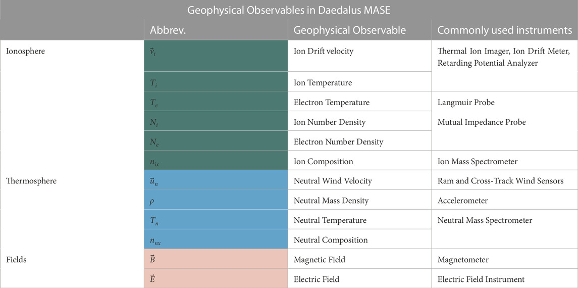
TABLE 1. List of primary products or geophysical observables in Daedalus MASE and commonly used instruments for their derivation.

For demonstrations and examples of Daedalus MASE functionality herein, data are obtained from global self-consistent simulations of the comprehensive LTI environment, obtained through NCAR’s TIEGCM. Primary observable time series are extracted from TIEGCM grids through interpolation along realistic orbit tracks, with user-defined errors representing instrument and/or measurement errors and/or estimated through external user-specified parametric instrument simulators.

Daedalus MASE is composed as a set of modules written in Python, each of which can be used as a stand-alone package. These modules are accompanied by Jupyter Notebooks: a Jupyter Notebook is an open-source web application that integrates in a comprehensive way code, the underlying equations and theory, the output of computations performed by the code, visualizations of the code results (including 2D and 3D plots, projections on a sphere, along-orbit plots, etc), and multiple other multimedia resources, along with explanatory text. These are all provided in a single repository, allowing scientists to easily access all elements of the programming process.

An overview of the repository, named DaedalusMASE, is presented in Figure 1. The repository is publicly available as a GitHub package, and can be downloaded at: https://github.com/DaedalusMASE/DaedalusMASE. In its current form, DaedalusMASE is built in the form of six main modules. These are: a) derived_products module, used for the calculation of the derived products; b) collision_frequencies module, which implements different models of ion-neutral collision frequencies related to different models of interaction cross-sections; c) interpolation module, which is used for interpolation of TIEGCM parameters along a satellite orbit; d) error_propagation module, which is used for the estimation of instrumental errors on the derived products; e) coverage_calculator module, which estimates the coverage of regions of interest of the Daedalus mission; and f) global_statistics module, which investigates quantitatively whether the dataset of a variable obtained via an in situ sampling scheme is statistically significant. Each of the modules contains a folder with the corresponding source code, a documentation folder which includes the API documentation of the source code in. html format, and a folder which includes Jupyter notebooks that can be used either as stand-alone simulation tools or as tutorials on the use of each module. The DaedalusMASE repository includes also a folder with sample data, which contains input data needed by the modules, such as TIEGCM NetCDF files from a sample run, the corresponding geomagnetic indices, and sample orbital data.

FIGURE 1

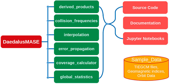
FIGURE 1. Overiview of the modules and structure of the Daedalus MASE repository.

Further to the above modules comprising Daedalus MASE, below we also present a set of Python routines that are used for the visualization of 3D datasets of GCMs. The visualization is performed using the Blender software package, and the code presented herein allows integrating the outputs of GCM model results, which are in the form of NetCDF files, with Blender, for creating the meshes and textures in 3D plots and animations. The repository is publicly available as a GitLab package, and can be downloaded at: https://gitlab.com/eelcodoornbos/blender_gcm_slices.

In the following we outline the functionality of each of the tools and modules comprising Daedalus MASE, based on processing of the above primary products listed in Table 1.

2.1 Daedalus MASE derived products module

One of the main purposes of Daedalus MASE, and indeed an overarching theme of the Daedalus mission, is to explore ion-neutral interaction processes within the LTI, focusing in particular on processes within the 100–200 km altitude range. Ion-neutral interaction processes within this region require simultaneous and co-located measurements of all relevant parameters in order to be resolved quantitatively, and these measurements can only be provided in situ by a spacecraft equipped with all relevant instruments. The goal of this module is to demonstrate the quantification of key physical processes related to ion-neutral interactions. These physical processes are directly linked to a list of quantities that can be derived analytically from the geophysical observables listed in Table 1. These are listed in Table 2 and are classified in terms of: a) heating sources, b) conductivity/cross-sections/collision frequencies, and c) electrical currents/magnetospheric forcing in the LTI, and are discussed in further detail below.

TABLE 2

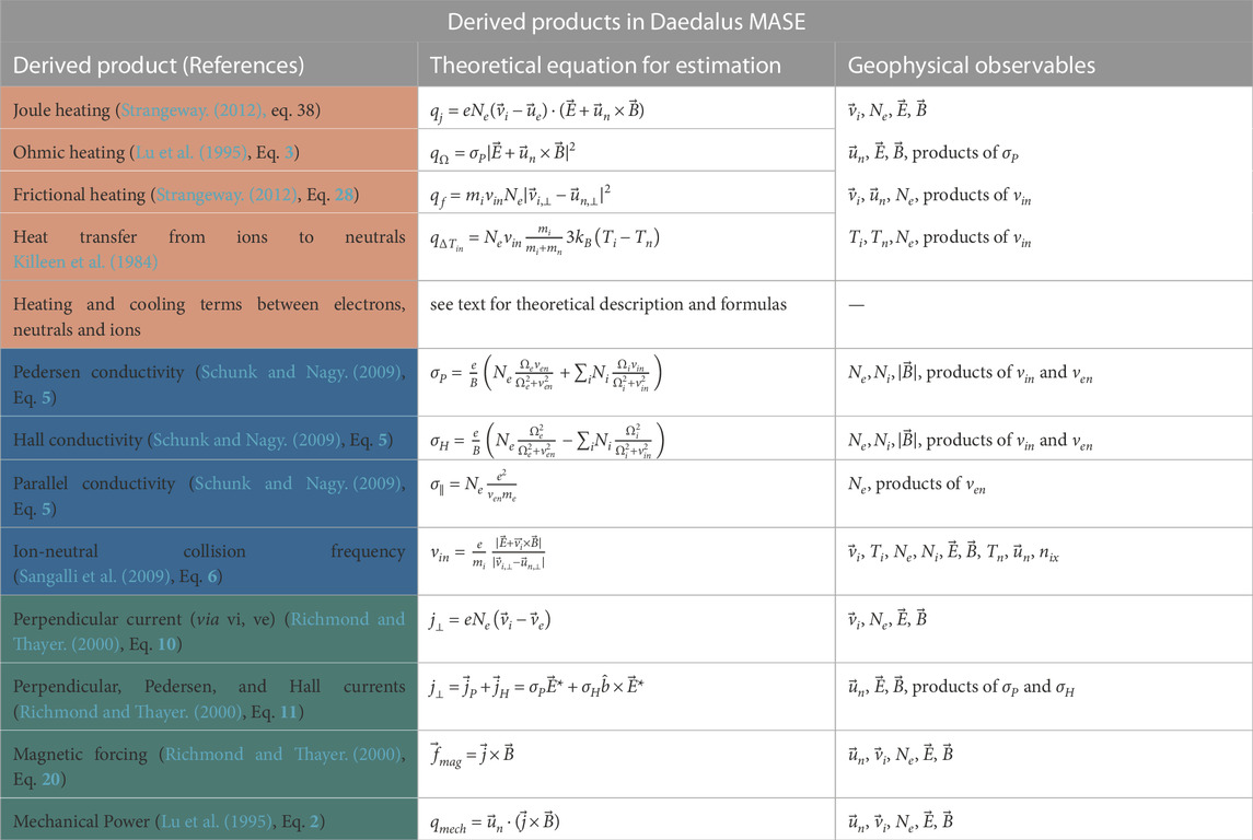
TABLE 2. List of derived products in Daedalus MASE and contributing primary observables.

Calculations of the derived products are performed with the daedalusmase_derived_products package of DaedalusMASE, which is composed of a series of modules and sub-modules, as detailed in Supplementary Tables S1–S7. In the following we present the corresponding routines that comprise these modules, along with analytic theoretical descriptions of the formulas and the assumptions used. In the folder Jupyter_Notebooks of the repository, there are example codes in the form of Jupyter notebooks which demonstrate the use of the routines.

2.1.1 Heating sources module

The first set of derived products in Table 2, marked in red, lists key heating sources and heat transfer processes in the LTI. In particular, a recurring unknown quantity of great significance in the energy budget of the LTI is Joule, or frictional, or Ohmic heating rate, and how it drives or evolves in concert with the plasma and neutral dynamics; at the same time, characterizing the variability of Joule heating within the latitude and altitude region where it maximizes is a critical missing piece in LTI processes. In further detail:

2.1.1.1 Joule, frictional, and ohmic heating rates

Joule heating (q_j) (Strangeway. (2012), eq. 38) and the relevant equivalent expressions for frictional heating (q_f) (Strangeway. (2012), Eq. 28) and Ohmic heating (q_Ω) (Lu et al. (1995), Eq. (3)) provide three distinct estimation methods of the same local energy dissipation process viewed from different perspectives, and are expected to yield similar values. Estimating all three provides redundancy, by partially relying on different inputs, but with anticipated differences in performance as a function of altitude. They also enable a cross-comparison providing confirmation of the physics at play. Joule heating is given by equation:

$q_j={\vec{J}}_{\perp }\cdot \vec{E}*=e{N}_e\left({\vec{v}}_{i,\perp }-{\vec{u}}_{e,\perp }\right)\cdot \left(\vec{E}+{\vec{u}}_n\times \vec{B}\right)(1)$

where e is the electron charge, N_e is the electron number density, ${\vec{v}}_{i,\perp }$ and ${\vec{u}}_{e,\perp }$ are the ion and electron velocities perpendicular to the geomagnetic field, ${\vec{J}}_{\perp }=e{N}_e({\vec{v}}_{i,\perp }-{\vec{u}}_{e,\perp })$ is the electric current perpendicular to the geomagnetic field, $\vec{E}$ the electric field, $\vec{B}$ the magnetic field, ${\vec{u}}_n$ the bulk velocity of the neutrals, and $\vec{E}*=\vec{E}+{\vec{u}}_n\times \vec{B}$ is the electric field in the reference frame of the neutrals.

At altitudes where ν_en ≪Ω_e, the electrons are magnetized, thus they move at a velocity (in the neutral reference frame):

${\vec{v}}_{e\perp }^{*}\approx \frac{\vec{E}*\times \vec{B}}{B^2}(2)$

which in the satellite rest frame is:

${\vec{v}}_{e\perp }\approx {\vec{u}}_n+\frac{\left(\vec{E}+{\vec{u}}_n\times \vec{B}\right)\times \vec{B}}{B^2}(3)$

This is valid at all ionospheric heights above the D region ($>$90 km).

The parallel electron mobility is large enough to produce a very large parallel conductivity σ_‖ compared to the Pedersen and Hall conductivities, σ_P and σ_H, respectively, which means that the electrons generally move more easily along the magnetic field. This means that they tend to sort out any field-aligned (i.e. parallel to the magnetic field) electric fields, and thus, that the electric field tends to be perpendicular to the magnetic field, or else that:

${\vec{E}}_{\Vert }=0(4)$

Inserting Eq. 3 and Eqs 4–1:

$q_j=e{N}_e\left({\vec{v}}_i^{*}-{\vec{v}}_e^{*}\right)\cdot {\vec{E}}_{\perp }*=e{N}_e\left({\vec{v}}_i-{\vec{v}}_e\right)\cdot \left({\vec{E}}_{\perp }+{\vec{u}}_n\times \vec{B}\right)(5)$

$q_j=e{N}_e\left[{\vec{v}}_i-\left(\frac{{\vec{E}}_{\perp }+{\vec{u}}_n\times \vec{B}}{B^2}+{\vec{u}}_n\right)\right]\cdot \left({\vec{E}}_{\perp }+{\vec{u}}_n\times \vec{B}\right)(6)$

using the identity $(\vec{a}\times \vec{c})\cdot \vec{a}=0$, this reduces to:

$q_j=e{N}_e\left({\vec{v}}_i-{\vec{u}}_n\right)\cdot \left({\vec{E}}_{\perp }+{\vec{u}}_n\times \vec{B}\right)=e{N}_e{\vec{v}}_{i\perp }^{*}{\vec{E}}_{\perp }*(7)$

meaning that the Joule heating rate can be estimated by the ion current times the electric field. For an ion population that consists of i species with N_i number densities, where $i=O_2^{+},N{O}^{+},O^{+},\dots$, Eq. 7 becomes:

$q_j=e\sum _{i=O_2^{+},N{O}^{+},O^{+},\dots }{N}_i{\vec{v}}_i\left({\vec{E}}_{\perp }+{\vec{u}}_n\times \vec{B}\right)(8)$

where:

$N_e=\sum _{i=O_2^{+},N{O}^{+},O^{+},\dots }{N}_i(9)$

The expression for Ohmic heating is given as:

$q_{\mathrm{\Omega }}={\sigma }_P{\left(\vec{E}+{\vec{u}}_n\times \vec{B}\right)}^2(10)$

The frictional heating rate is calculated as:

$q_f=m_i{\nu }_{in}{N}_e|{\vec{v}}_{i,\perp }-{\vec{u}}_{n,\perp }{|}^2(11)$

where m_i is the ion mass and ν_in is the ion-neutral collision frequency.

Joule, frictional and Ohmic heating rates in Daedalus MASE are calculated by the joule, frictional and ohmic routines of the daedalusmase_derived_products.mod_heating_sources.sub_heating_rates sub-module.

2.1.1.2 Convection and wind heating

By expanding Eq. 10 for Ohmic heating, we obtain:

$\begin{array}{ll}\hfill q_{\mathrm{\Omega }}& ={\sigma }_P{\left(\vec{E}+{\vec{u}}_n\times \vec{B}\right)}^2\hfill \\ \hfill & =\underset{q_c}{\underbrace{{\sigma }_P{E}^2}}+\underset{q_w}{\underbrace{{\sigma }_P|{\vec{u}}_n\times \vec{B}{|}^2-2{\sigma }_P{\vec{u}}_n\cdot \left(\vec{E}\times \vec{B}\right)}}\hfill \end{array}(12)$

In this formula, the first term marked as q_c is known as convection heating [Lu et al. (1995); Billett et al. (2018)], and corresponds to the Joule heating rate in the absence of neutral winds, whereas the second term marked as q_w is the neutral wind correction term (Billett et al., 2018), often termed “wind heating” (Lu et al., 1995), which gives a measure of the error in estimating Joule heating rate neglecting neutral winds. When neutral winds are driven frictionally by $\vec{E}\times \vec{B}$ convection, e.g., during substorm growth and expansion phases, the presence of neutral winds has in general the tendency to lower the convection heating, thus an estimation of Joule heating without taking into account the presence of neutral winds will lead to an over-estimation. On the other hand, when neutral winds have a dynamo effect, e.g., during substorm recovery (when $\vec{E}\times \vec{B}$ convection decreases, while the inertia of the massive neutral atmosphere supports the neutral winds a longer time), this is no longer true. Whereas numerous studies have shown that the neutral winds can affect Joule heating substantially [Lu et al. (1995); Thayer. (1998); Deng and Ridley. (2007)], the quantification of the contribution of the neutral winds requires detailed measurements of all relevant parameters. This module enables the separate computation and cross-comparison of the two terms, both in models and in cases that in situ measurements are available.

Convection and wind heating rates in Daedalus MASE are calculated by the convection_heat and wind_heat routines of the daedalusmase_derived_products.mod_heating_sources.sub_heating_rates sub-module.

2.1.1.3 Ohmic heating per unit mass

Also related to the heating sources is the estimate of Ohmic heating per unit mass. The rate of local temperature change in the thermosphere due to Joule heating is more directly related to the heating per unit mass, i.e., the volumetric heating rate divided by the mass density. This is because, although the volumetric heating is decreasing with altitude, the mass density decreases more rapidly, and thus less energy is required to significantly heat the more tenuous neutral gas (Richmond and Thayer, 2000). Thus, whereas the volumetric heating rate is largest in the E region, the heating per unit mass becomes larger higher up, in the F region. This is calculated according to:

$q_{j,\rho }=\frac{{\sigma }_P{\left(\vec{E}+{\vec{u}}_n\times \vec{B}\right)}^2}{\rho }(13)$

where ρ is the neutral density.

Ohmic heating rate per unit mass in Daedalus MASE is calculated by the ohmic_per_mass routine of the daedalusmase_derived_products.mod_heating_sources module.

2.1.1.4 Ratio of joule heating over pressure

This module also enables the calculation of the ratio of Joule heating over pressure. This ratio has units of 1/s (since Joule heating has units of W = kg⋅m²s⁻³, and atmospheric pressure has units of Pa = kgm⁻¹s⁻²), and provides an indication of the time until the accumulated Joule heating in a certain volume would equal the thermal energy that is present in that volume of the atmosphere in absence of convection and heat conduction.

The ratio of Joule heating over pressure in Daedalus MASE is calculated by the ohmic_per_pressure routine of the daedalusmase_derived_products.mod_heating_sources module.

2.1.1.5 Heat transfer rates between species

The routines of the daedalusmase_derived_products.mod_heating_sources. sub_heat_transfer_rates sub-module enable the calculation of the heat transfer rates between species, such as the heat transfer rates from ions to neutrals, electrons to neutrals and ions to/from electrons. It is noted that the friction between ions and neutrals as well as ionization result in different temperatures of ions, electrons and the neutral gas, and heat transfer due to elastic collision between these species. The rates can be derived from observed temperatures and collision frequencies. When different temperatures between ions and neutrals are observed, then the heat transfer between the two species can be estimated according to Killeen et al. (1984) as:

$q_{\mathrm{\Delta }{T}_{in}}=N_e{\nu }_{in}\frac{m_i}{m_i+m_n}3k_B\left(T_i-T_n\right)(14)$

Similarly, for the ion-electron case:

$q_{\mathrm{\Delta }{T}_{ie}}=N_e{\nu }_{ie}\frac{m_i}{m_i+m_e}3k_B\left(T_i-T_e\right)(15)$

and for the electron-neutral case:

$q_{\mathrm{\Delta }{T}_{en}}=N_e{\nu }_{en}\frac{m_e}{m_e+m_n}3k_B\left(T_e-T_n\right)(16)$

where subscripts i, e and n denote ions, neutrals and electrons respectively, T, ν and m denote temperatures, collision frequencies and masses, respectively, for each species, and k_B is the Boltzmann constant.

In general, T_e and T_i are greater than T_n, thus a heat transfer from electrons and ions to the neutrals is observed. On the other hand, although in general T_e > T_i, at very low altitudes and/or during disturbed geomagnetic conditions, T_i can exceed T_e locally. In this case the heat flow between ions and electrons is reversed and the electrons are heated.

Heat transfer from ions to neutrals is calculated by the heat_transfer_in routine, and from electrons to neutrals by the heat_transfer_en_elastic routine. Finally, the energy exchange between ions and electrons is calculated by the heat_transfer_ei routine of the daedalusmase_derived_products.mod_heating_sources. sub_heat_transfer_rates sub-module.

2.1.1.6 Frictional heating rates

Frictional heating arises due to the differential velocity between species. Whereas with Eq. 11, we calculated the total ion-neutral frictional heating (q_f), here we calculate the frictional heating between each individual ion and neutral species. Furthermore, we calculate frictional heating between ions and electrons and between different ion species. The frictional heating rate between ions and neutrals is given as:

$q{F}_{in}=N_i{m}_i\sum _n\frac{{\nu }_{in}{m}_n{\left(u_n-u_i\right)}^2}{m_i+m_n}(17)$

The frictional heating rate between ions and electrons is:

$q{F}_{ie}=N_e{m}_e\sum _i\frac{{\nu }_{ei}{m}_i{\left(u_e-u_i\right)}^2}{m_i+m_e}(18)$

The frictional heating rate between different ion species is:

$q{F}_{ij}=N_j{m}_j\sum _i\frac{{\nu }_{ji}{m}_i{\left(u_j-u_i\right)}^2}{m_i+m_j}(19)$

where N refers to number density, m is the mass, ν is the collision frequency and u is the velocity. Subscripts i, j refer to different ion species, e denotes electrons, n denotes neutrals.

It is noted that the sub-module named sub_frictional_heating_rates includes an extensive set of routines for calculating the corresponding heating rates separately for O⁺, $O_2^{+}$, NO⁺ and N⁺ ions. This allows the contribution of various species to the total heating to be evaluated.

2.1.1.7 Electron cooling rates

The daedalusmase_derived_products.mod_heating_sources. sub_cooling_rates sub-module includes routines for the calculation of inelastic collisions between electrons and neutrals. Specifically, includes routines for calculating electron losses due to N₂ rotational [sub_colling_rates.N2_rot] and vibrational [sub_colling_rates.N2_vib] excitation, O₂ rotational [sub_colling_rates.O2_rot] and vibrational [sub_colling_rates.O2_vib] excitation and O fine structure [sub_colling_rates.O_fine]. The relevant formulas can be found in Schunk and Nagy. (2009).

2.1.2 Conductivities module

Module daedalsumase_derived_products.mod_conductivities includes routines for the calculation of Pedersen (σ_P), Hall (σ_H) and parallel (σ_‖) conductivities as described in Richmond and Thayer. (2000), using the following equations (see also Table 2):

$\begin{array}{ll}\hfill {\sigma }_P& =\frac{e}{B}\left(N_e\frac{{\mathrm{\Omega }}_e{\nu }_{en}}{{\mathrm{\Omega }}_e^2+{\nu }_{en}^2}+\sum _i{N}_i\frac{{\mathrm{\Omega }}_i{\nu }_{in}}{{\mathrm{\Omega }}_i^2+{\nu }_{in}^2}\right)\hfill \\ \hfill & =\frac{e}{B}\left(N_e\frac{{\kappa }_e}{1+{\kappa }_e^2}+\sum _i{N}_i\frac{{\kappa }_i}{1+{\kappa }_i^2}\right)\hfill \end{array}(20)$

$\begin{array}{ll}\hfill {\sigma }_H& =\frac{e}{B}\left(N_e\frac{{\mathrm{\Omega }}_e^2}{{\mathrm{\Omega }}_e^2+{\nu }_{en}^2}-\sum _i{N}_i\frac{{\mathrm{\Omega }}_i^2}{{\mathrm{\Omega }}_i^2+{\nu }_{in}^2}\right)\hfill \\ \hfill & =\frac{e}{B}\left(N_e\frac{{\kappa }_e^2}{1+{\kappa }_e^2}-\sum _i{N}_i\frac{{\kappa }_i^2}{1+{\kappa }_i^2}\right)\hfill \end{array}(21)$

${\sigma }_{\Vert }=N_e\frac{e^2}{{\nu }_{en}{m}_e}(22)$

where ν_en is the electron neutral collision frequency, Ω_e and Ω_i are the electron and ion gyrofrequencies respectively, e is the electron charge, N_e is the electron number density, N_i is the ion number density and κ_i is the ratio of the gyrofrequency over the collision frequency of each ion.

The Pedersen conductivity is calculated by the routine pedersen_cond, the Hall conductivity is calculated by the routine hall_cond and the parallel conductivity is calculated by the routine parallel_cond.

2.1.3 Collision frequencies and cross sections module

Conductivities, collision cross-sections and collision frequencies, are key parameters that affect heating in the LTI, and are also critical in both LTI and magnetosphere modelling. In the Earth’s LTI system, the interactions of ions and neutrals influence the velocities, temperatures and densities of both species, thus playing a vital role in momentum and energy exchange between the thermosphere and the ionosphere. These interactions are characterised through the ion neutral collision frequencies and subsequently (fundamentally) through the ion-neutral cross sections, which are fundamental parameters in the coupling between the neutral atmosphere and the ionosphere. However, collision cross-sections, as documented in, e.g., Schunk and Nagy. (2009); Richmond. (2017), have been determined primarily through laboratory experiments, which are not necessarily representative of the real LTI environment, and are believed to have systematic biases.

2.1.3.1 Collision frequencies

The mod_collision_freqs_cross_sections.sub_collision_frequencies sub-module includes routines for the calculations of the collision frequencies between electrons, ions and neutrals. The laboratory-derived relevant formulas can be found in Schunk and Nagy. (2009). For the case of ion-neutral collisions, another option is to use the ion momentum equation (Sangalli et al. (2009); Sarris et al. (2020)) in order to derive the corresponding collision frequency. The ion momentum equation is given as:

$\begin{array}{ll}\hfill m_i{N}_i\left(\frac{\partial }{\partial t}+\overrightarrow{v_i}\nabla \right){\vec{v}}_i& =q_i{N}_i\left(\vec{E}+{\vec{u}}_i\times \vec{B}\right)-m_i{N}_i{\nu }_{in}\left({\vec{v}}_i-{\vec{u}}_n\right)\hfill \\ \hfill & -m_i{N}_i{\nu }_{ie}\left({\vec{v}}_i-{\vec{v}}_e\right)+m_i{N}_i\vec{g}-\nabla P_i\hfill \end{array}(23)$

where q_i id the ion charge, $\vec{g}$ is the gravity acceleration and P_i is the ion thermal pressure. Assuming a homogenous plasma and neglecting gravity and pressure contributions:

$\begin{array}{ll}\hfill m_i{N}_i\frac{\partial }{\partial t}{\vec{v}}_i& =q_i{N}_i\left(\vec{E}+{\vec{u}}_i\times \vec{B}\right)-m_i{N}_i{\nu }_{in}\left({\vec{v}}_i-{\vec{u}}_n\right)\hfill \\ \hfill & -m_i{N}_i{\nu }_{ie}\left({\vec{v}}_i-{\vec{v}}_e\right)\hfill \end{array}(24)$

Taking the expression for motion perpendicular to the geomagnetic field and assuming a steady state:

$\begin{array}{ll}\hfill 0& =q_i{N}_i\left({\vec{E}}_{\perp }+{\vec{u}}_i\times \vec{B}\right)-m_i{N}_i{\nu }_{in}\left({\vec{v}}_{i,\perp }-{\vec{u}}_{n,\perp }\right)\hfill \\ \hfill & -m_i{N}_i{\nu }_{ie}\left({\vec{v}}_{i,\perp }-{\vec{v}}_{e,\perp }\right)\hfill \end{array}(25)$

Collisions between electrons and ions become important (relatively to ion-neutral collisions) only in the upper ionosphere, where, though, ions and electrons have almost same velocities perpendicular to $\vec{B}$ (E × B drift), thus ${\vec{v}}_{i,\perp }-{\vec{v}}_{e,\perp }\approx 0$ and we can neglect the third term on the right-hand side of Eq. (26):

$q_i{N}_i\left({\vec{E}}_{\perp }+{\vec{u}}_i\times \vec{B}\right)=m_i{N}_i{\nu }_{in}\left({\vec{v}}_{i,\perp }-{\vec{u}}_{n,\perp }\right)(26)$

Finally, solving for ν_in, yields:

${\nu }_{in}=\frac{q_i}{m_i}\frac{|{\vec{E}}_{\perp }+\overrightarrow{v_i}\times \vec{B}|}{|{\vec{v}}_{i,\perp }-{\vec{u}}_{n,\perp }|}(27)$

2.1.3.2 Cross sections

Subsequently, mod_collision_freqs_cross_sections.sub_cross_sections sub-module calculates ion-neutral cross sections according to Banks and Kockarts. (1973) using the following formula:

${\sigma }_{in}=\frac{{\nu }_{in}}{N_n\sqrt{\frac{2k_B{T}_i}{m_i}}}(28)$

2.1.4 Currents and magnetic forcing module

An open question in the lower thermosphere and ionosphere is how atmospheric and magnetospheric forcing and drag between charged and neutral species affect the wind structure, convection patterns, and electric currents in the region. To this direction, the third set of derived products, marked in green in Table 2, includes calculations of currents flowing perpendicularly to the magnetic field. Perpendicular currents are calculated both through the differential velocity between ion drift and electron drift (given by E × B in the LTI) and through the Hall and Pedersen currents. The magnetic forcing, i.e. the Lorentz force, that plasma exerts on the neutral atmosphere through collisional coupling, is also listed. The perpendicular currents and magnetic forcing are calculated by module mod_currents_magnetic_forcing, as discussed in further detail in the corresponding sections below.

2.1.4.1 Current density

Within the lower ionosphere, Pedersen currents flow in the direction of the electric field, while the Hall currents flow in the direction opposite to the $\vec{E}\times \vec{B}$ direction, i.e. perpendicularly to the electric and the magnetic field. Pedersen currents flow a bit higher (∼ 120 km) where the Pedersen conductivity maximizes, whereas the Hall currents flow lower, at the altitude where the Hall conductivity maximizes (i.e., ∼ 115 km). The problem is that the current density ${\vec{j}}_{\perp }$ cannot be determined directly; ${\vec{j}}_{\perp }$ can be, in principle, inferred from magnetometer data, which is, however, not straightforward at altitudes where Pedersen, Hall and field-aligned currents co-exist and all contribute to the local magnetic field, i.e., roughly below 300 km. Alternatively, assuming quasi-neutrality, i.e., that the electron density N_e is equal to the sum of the ion species densities $N_{O^{+}}$, $N_{O{2}^{+}}$, and $N_{N{O}^{+}}$, and denoting the electron and ion drifts for each species with v_e, $v_{O^{+}}$, $v_{O_2^{+}}$, and $v_{N{O}^{+}}$, respectively, we can calculate the perpendicular currents by using:

$\begin{array}{ll}\hfill {\vec{j}}_{\perp }& =e\left(N_{O^{+}}{\vec{v}}_{O^{+}}+N_{O{2}^{+}}{\vec{v}}_{O_2^{+}}+N_{N{O}^{+}}{\vec{v}}_{N{O}^{+}}\right.\hfill \\ \hfill & \left.+N_{N^{+}}{\vec{v}}_{N^{+}}-N_e{\vec{v}}_e\right)\hfill \\ \hfill & \approx e{N}_e\left({\vec{v}}_i-{\vec{v}}_e\right)\hfill \end{array}(29)$

Another way to calculate the perpendicular currents is by using Ohm’s law. From that perspective one can calculate the Pedersen and Hall components of the perpendicular currents independently as follows:

${\vec{j}}_{\perp }={\sigma }_P\vec{E}*+{\sigma }_H\widehat{b}\times \vec{E}*={\vec{j}}_P+{\vec{j}}_H(30)$

where σ_H is the Hall conductivity, $\widehat{b}$ is the unit vector of the magnetic field, the perpendicular sign refers to quantities perpendicular to the magnetic field and the star sign denotes the electric field in the reference frame of the neutrals:

$\vec{E}*={\vec{E}}_{\perp }+{\vec{u}}_n\times \vec{B}(31)$

The Pedersen current is calculated by the routine current_pedersen, the Hall current is calculated by the routine current_hall and the perpendicular current is calculated by the routine current_perp of the mod_currents_magnetic_forcing module.

2.1.4.2 Magnetic forcing

The closure of currents in the magnetosphere and in the ionosphere produces a ${\vec{j}}_{\perp }\times \vec{B}$ force at each region. In the magnetosphere this force can slow down the magnetospheric convection and provide energy to the electromagnetic field, thus acting like a dynamo/generator that converts kinetic energy to electromagnetic energy; it is noted that in the magnetosphere one can also encounter motor/load regions, where plasma is accelerated (e.g., at reconnection sites). In the ionospheric counterpart, the ${\vec{j}}_{\perp }\times \vec{B}$ force balances the frictional drag on the ions by the neutral atmosphere preserving the ionospheric convection and consequently accelerates the neutrals in the direction of the plasma flow. The ${\vec{j}}_{\perp }\times \vec{B}$ force in the ionosphere consists of two components associated with the Pedersen and Hall currents. The Pedersen associated part, counteracts the drag force in the direction opposite to the $\vec{E}\times \vec{B}$ direction, while the Hall part balances the drag force in the direction of the electric field. Equal and opposite forces act also on the neutrals, which tend to drive neutral winds in the Thermosphere. Although the ${\vec{j}}_{\perp }\times \vec{B}$ part associated with the Pedersen current is of the same order as the Hall associated part, as the Pedersen currents flow higher than the Hall currents, the neutral density in the region is lower and thus are more efficient in driving neutral winds (Cowley, 2000). Daedalus MASE allows the investigation of the altitude-dependent contribution of the Pedersen and Hall currents in the total ${\vec{j}}_{\perp }\times \vec{B}$ forcing term.

In order to address the coupling between the thermosphere, the ionosphere and the magnetosphere, we apply Poynting’s theorem to the entire system [e.g., Thayer and Vickrey. (1992); Lu et al. (1995)]:

$\frac{\partial w}{\partial t}+\nabla \cdot \left(\frac{\vec{E}\times \vec{B}}{{\mu }_0}\right)+\vec{j}\cdot \vec{E}=0(32)$

where w is the electromagnetic energy density, μ₀ is the magnetic permeability of free space and $\vec{J}$ is the current density. Assuming a steady state (i.e., assuming that the change of the total electromagnetic energy in time can be ignored compared to the plasma motion), Eq. 32 becomes:

$\nabla \cdot \left(\frac{\vec{E}\times \vec{B}}{{\mu }_0}\right)+\vec{j}\cdot \vec{E}=0(33)$

where the first term is the divergence of the electromagnetic energy flux, and the second term is the energy transfer rate. As explained above (see Eq. 4) the electric field component perpendicular to the geomagnetic field $({\vec{E}}_{\perp })$ is much larger than the parallel component $({\vec{E}}_{\Vert })$, thus $\vec{J}\cdot \vec{E}$ roughly equals ${\vec{J}}_{\perp }\cdot {\vec{E}}_{\perp }$. Further analyzing the energy transfer rate leads to:

${\vec{j}}_{\perp }\cdot {\vec{E}}_{\perp }=\underset{q_j}{\underbrace{{\vec{j}}_{\perp }\cdot \vec{E}*}}+\underset{ϵ}{\underbrace{{\vec{u}}_n\cdot \left({\vec{j}}_{\perp }\times \vec{B}\right)}}(34)$

where ϵ is the mechanical power exerted on the neutrals by the ${\vec{j}}_{\perp }\times \vec{B}$ forcing (Lu et al., 1995) and $\vec{E}*$ is the electric field in the neutral wind reference frame (Eq. 31).

The ${\vec{j}}_{\perp }\times \vec{B}$ forcing is calculated by the routine JxB_forcing and the mechanical power by the routine mechanical_power of the mod_currents_magnetic_forcing module.

2.1.5 TIEGCM utilities module

Apart from the modules for the calculation of the various derived products as discussed above, daedalusmase_derived_products includes several routines for processing TIEGCM outputs, combined into the tiegcm_utils module. Specifically, the read_tiegcm routine is used for reading TIEGCM output files, which by default are in Network Common Data Form (NetCDF) format. The convert_mmr routine is used to convert TIEGCM densities from mass mixing ratio (mmr) to cm⁻³. Furthermore, the igrf_B routine is used for the calculation of the IGRF magnetic field and the electric_field routine for the calculation of the electric field from $\vec{E}\times \vec{B}$ velocities.

It is noted that TIEGCM does not solve the ion momentum equations explicitly to calculate the ion velocities; instead, the ion velocities are calculated in post processing by using subroutine tgcmproc, which can be found in the list of TIEGCM post-processors available from NCAR, written in Fortran. In a similar manner, DaedalusMASE uses the ion and electron momentum equations to derive expressions for the ion and electron velocities. By neglecting the forces due to pressure gradient and gravity, the ion and electron velocities can be given as ((Richmond and Thayer, 2000):

${\vec{v}}_{i\perp }*=\frac{{\nu }_{in}{\mathrm{\Omega }}_i{\vec{E}}_{\perp }*-{\mathrm{\Omega }}_i^2\widehat{b}\times {\vec{E}}_{\perp }*}{B\left({\nu }_{in}^2+{\mathrm{\Omega }}_i^2\right)}(35)$

and

${\vec{v}}_{e\perp }^{*}=\frac{-{\nu }_{en}{\mathrm{\Omega }}_e{\vec{E}}_{\perp }^{*}-{\mathrm{\Omega }}_e^2\widehat{b}\times {\vec{E}}_{\perp }^{*}}{B\left({\nu }_{en}^2+{\mathrm{\Omega }}_e^2\right)}(36)$

where the star sign denotes the corresponding velocities and electric field in the neutral wind reference frame. Module tiegcm_utils includes routines for the calculation of e, O⁺, $O_2^{+}$, NO⁺ and N⁺ velocities.

2.1.6 Height integration module

Using inputs from the locally-computed derived products in TIEGCM, as described in the section above and listed in Table 2, this module enables also the calculation of height-integrated and hemispherically-integrated derived products. Such estimates are of particular importance for LTI processes, as, for example, in order to provide a quantitative assessment of high-latitude energy input, the hemispherically-integrated Joule heating in the Northern or Southern hemispheres needs to be estimated [e.g., Deng et al. (2009)]. Several previous studies have also studied Joule heating in two dimensions, corresponding to the altitude-integrated Joule heating [Thayer. (1998); Lu et al. (1995); Weimer. (2005); Deng et al. (2009)]. Furthermore, estimations of the height-integrated Pedersen conductivities in the E (100–150 km) and F (150–600 km) regions and their ratio has been used to obtain an estimate of the ratio of the Joule heating deposited in the E and F regions (Sheng et al., 2014).

Whereas height-integrated estimations of various products are commonly used in processing GCM outputs, there is a lack of an open-source tool that enables the computation of integrations with user-defined limits. This module enables the integration of GCM gridded data over a user-specified latitude and longitude, and also enables producing latitude-longitude maps of height-integrated Joule heating, Pedersen conductance (height-integrated Pedersen conductivity), Hall conductance (height-integrated Hall conductivity), and height-integrated Pedersen and Hall currents. Height integrations are performed with a trapezoidal integration scheme, according to:

${\int }_a^{b}f\left(x\right)dx=\sum _{k=1}^N\frac{f\left(x_{k-1}\right)+f\left(x_k\right)}{2}\mathrm{\Delta }x(37)$

where f is the altitude-resolved quantity being integrated, x is the altitude, a and b are the upper and lower limits of integration, and k corresponds to the discrete levels where property f is provided. It is noted that most commonly in GCMs properties are calculated in terms of pressure levels; thus Δx_k is not fixed, but rather increases with altitude. Height integration in Daedalus MASE is performed with the integration_height routine of the daedalusmase_derived_products module.

In cases where height integration needs to be performed for a discrete altitude interval as opposed to the entire altitude range in a GCM (e.g., for the E region, at 100–150 km), the module performs a re-gridding process by interpolating the property under height-integration at user-defined altitude ranges of fixed length. This enables the subsequent integration to be performed over the same altitude range, rather than integrating over the same number of pressure levels, in which case the altitude range would be variable throughout the globe. The regridding procedure is performed by the regrid routine, while the integration with user defined latitude, longitude and altitude limits is performed by the integration routine of the module. In the Jupyter_Notebooks folder of the Daedalus MASE repository there are two notebooks for the demonstration of the use of this module: the daedalusmase_derived_products_regrid performs the regridding procedure for a TIEGCM NetCDF file, and the daedalusmase_derived_products_integration calculates the heating (joule, convection or wind) in GW that is confined inside a user defined 3D region of the thermopshere.

Height (and 3D) integration in geographic coordinates is particularly useful for calculating global or hemispherical energy inputs; it is noted, however, that many LTI phenomena are organised with respect to the geomagnetic field lines, due to the strong impact of the geomagnetic field on the motion of charged particles [e.g., Richmond. (1995); Laundal and Richmond. (2017)]. Furthermore, in the ionosphere magnetic field lines are often assumed to be equipotential, and thus the electric potential equation can be simplified and solved as a two-dimensional problem over magnetic longitude and latitude. Field line integrated Hall and Pedersen conductivities (termed conductances) are also key quantities in studying magnetosphere-ionosphere coupling. Thus, for magnetically organized phenomena, such as ionospheric currents, a field-aligned integration scheme is more suitable and is a very useful feature of an LTI toolset. A relevant module performing integrations along magnetic field lines is not currently included in Daedalus MASE, but is planned to be included in subsequent versions.

2.1.7 Derived products plotting utilities module

The mod_plot_utils includes routines for the visualization of the daedalusmase_derived_products results. These include vertical profiles, map plots, polar plots for the scalar products and quiver plots for the vector products. Examples of module outputs are presented in Figure 3 of the Results section.

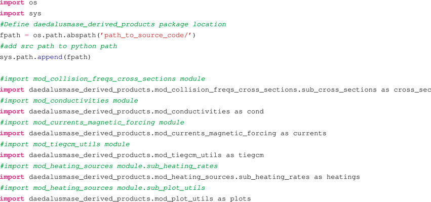
2.1.8 Importing daedalus MASE derived products modules

In order to import the modules, the user must add the daedalusmase_derived_products source code path to the Python path. This is done as follows: the built-in Python modules os and sys should be imported first. The os module implements functions on pathnames, while the sys module contains parameters specific to the system. The os. path.abspath() function is first used to define the path of the daedalusmase_derived_products folder which contains the source code of the package; subsequently the sys. path.append() function is used to add the source code path to the Python path. Then the modules can be imported to the code. In the following, we present a code snippet which illustrates this procedure:

2.2 Daedalus MASE collision frequencies module

In the Earth’s LTI system, the interactions of ions and neutrals influence the velocities, temperatures and densities of both species, thus playing a vital role in momentum transfer and energy exchange between the thermosphere and the ionosphere. These interactions are characterised through the ion neutral collision frequencies, ν_in, and subsequently (fundamentally) through the ion-neutral cross sections, σ_in. Ion-neutral collision frequencies depend on a number of terms, including the density and composition of the ion and neutral species, the ion and electron temperatures, and values for collision crosssections, σ_in; thus, through their effect on the determination of collision rates, collision cross-sections also affect Joule heating and conductivity estimations. Traditionally, collision cross-sections are obtained primarily through laboratory experiments of ion-neutral collisions and model extrapolations, and the resulting values for σ_in and ν_in are normally taken from published tables such as, for example, the tables in the text book by Schunk and Nagy. (2009). However, these estimations include large measurement uncertainties, and their accuracy has never been conclusively evaluated. The reason is that, whereas the microscopic processes underlying the estimation of σ_in are governed by fundamental physics, and whereas the underlying processes are the same in the laboratory environment and in the upper atmosphere, the observation conditions are largely different between the two environments, leading to different estimations, as the cross sections are not measured directly, but are rather inferred from macroscopic quantities. For example, laboratory experiments are not always performed under the similar conditions as in the ionosphere (e.g., they are often at lower temperatures, commonly around 300 K), leading to systematic uncertainties in both σ_in and ν_in in the upper atmosphere. The discrepancies are evident from comparisons of different estimates in the literature, such as between tables provided by Banks and Kockarts. (1973), Schunk and Nagy. (2009), and Richmond. (2017) and references therein. Due to the above discrepancies and uncertainties, collision cross-sections and collision rates are among the largest sources of errors in empirical models, GCMs and magnetosphere-ionosphere coupling simulations, to all of which they are key inputs. Together, the collision rates and collision cross sections represent the largest source of uncertainty in estimating the ionospheric conductivity, which is a key parameter in current coupled models of the LTI. Existing proxies of these parameters are based on semi-empirical relations and show large deviations due to lack of co-located measurements of all required parameters.

The E region of the Ionosphere, between 90 and 150 km approximately, is where electric currents perpendicular to the magnetic field (i.e., Pedersen and Hall currents) are mostly concentrated. These currents are the result of the relative velocities between electrons and ions. As electrons and ions interact with the neutrals their velocities deviate from the $\vec{E}\times \vec{B}$ drift which leads to different ion and electron velocities. Electrons are strongly bounded to the magnetic field, $\vec{E}\times \vec{B}$ drifting through this ionospheric altitude range, thus their interactions with neutrals (i.e., electron-neutral collision frequencies) are less important. On the other hand, the ions start to deviate from $\vec{E}\times \vec{B}$ at approximately 200 km and at the bottom of the E region are fully entrained by the neutrals, which indicates the significance of ion-neutral collision frequencies in the region. The dominant ion species in the region are $O_2^{+}$ and NO⁺ and the dominant neutral species are O, O₂ and N₂, thus the interactions between these species and the corresponding collision frequencies are the key parameters in the region, that affect the conductivity and the electric currents.

Further up, in the F region, between 150 and 500 km, O and O⁺ are the dominant constituents, thus the interactions between the two are crucial in determining the momentum and energy exchange between the ionosphere and the thermosphere (Salah, 1993). Moreover, the O−O⁺ momentum transfer collision cross sections are dominated by resonant charge exchange between O and O⁺, whereas the contribution from polarisation can be neglected in the F region (Banks, 1966). The importance of O−O⁺ collision frequency has been highlighted through many studies: for example, Moffett et al. (1990) researched the influence of O−O⁺ collision frequency on the behaviour of the ionospheric F region, and found that a 70% increase in the collision frequency increased the peak electron density by as much as 25% at nighttime and by 10% at daytime, while they also found an increase of the height of the maximum density by 20 km at night. Moreover, Roble. (1988) studied the influence of the collision frequency on the structure of the neutral atmosphere and found that a 70% increase in the atomic oxygen collision frequency led to an increase of the exospheric neutral temperature by 80 K at daytime, while the global averaged Joule heating was increased by 80%. However, while estimating the O−O⁺ cross section is crucial, it has never been measured directly in the LTI. Ion-neutral cross sections have been derived from laboratory measurements by extrapolation of the low-energy laboratory data to higher energies, although recent investigations indicate that these measurements might not be accurate or applicable (e.g., Archer et al. (2017)). Since the estimates of ion-neutral collision frequencies are currently not accurate and include large discrepancies, the assumptions that go into their estimations need to be well understood and the variations arising from different ion-neutral collision frequency models need to be considered.

Whereas in Section 2.1.3.1 we calculated ion-neutral collision frequencies based on the formula of Sangalli et al. (2009) and the theoretical formulas of Schunk and Nagy. (2009), here we use a set of different formulas for the calculation of collision frequencies found in literature. The daedalusmase_collision_frequencies package aims to provide a computational compendium of all estimation methodologies and parameterizations, allowing their cross-comparison while revealing their discrepancies, e.g. as a function of altitude or temperature, and the quantitative effect of these discrepancies in the calculation of the ionospheric conductivities. In the following we present the corresponding routines that comprise daedalusmase_collision_frequencies modules, along with analytic theoretical descriptions of the formulas used. A list of the routines along with corresponding description is presented in Supplementary Table S8. The package is accompanied by a Jupyter notebook, in the Jupyter_Notebooks folder, that can be used as a stand-alone simulation tool as well as a tutorial for the use of the module.

2.2.1 Collision frequencies module

The mod_collision_freqs module includes all the routines needed for the calculation of ion-neutral collision frequencies based on different models. In its current version the module includes routines for the calculation of the collision frequencies between O⁺, $O_2^{+}$ and NO⁺ ions and O, O₂ and N₂ neutral species, based on Banks. (1966) (vin_banks routine), Schunk and Walker. (1973) (vin_schunk_walker routine), Schunk and Nagy. (2009) (vin_schunk_nagy routine), Richmond. (2017) (vin_richmond routine) and Ieda. (2020) (vin_ieda routine). Especially, for the O⁺−O collision frequencies, op_o_cols routine includes the parameterizations and equations used in the studies by Dalgarno et al. (1964), Banks. (1966), Stubbe. (1968), Schunk and Walker. (1973), Salah. (1993), Pesnell et al. (1993), Hickman et al. (1997), Richmond. (2017), Schunk and Nagy. (2009) and Ieda. (2020). Furthermore and in order to access the impact of the differences of the ion-neutral collisions models on the conductivities, the module includes the routines pedersen and hall for the calculation of the Pedersen and Hall conductivities respectively.

2.2.2 Collision frequencies utilities module

The routines of the mod_collision_freqs module, need ion and electron temperatures, geomagnetic field, and ion, electron and neutral densities as inputs. These parameters, as was mentioned above, can be extracted either from GCMs or from empirical models. The mod_utils module, includes routines for running empirical models and extracting the needed parameters. More specifically, temperatures and densities of electrons and ions are derived from IRI 2016 (run_iri routine), the neutral temperature and densities from MSIS00 (run_msis routine) and the geomagnetic field from IGRF 2012 (run_igrf routine). Furthermore, this module includes the definitions of the needed constants for the calculations.

2.2.3 Collision frequencies plotting module

The mod_plot_utils includes routines for the visualization of the mod_collision_freqs module results. These include vertical profiles of collision frequencies and conductivities, as well as temperature dependence of collision frequencies. Figure 4 of the Results section, presents three example plots of the module.

2.2.4 Importing daedalus MASE collision frequencies modules

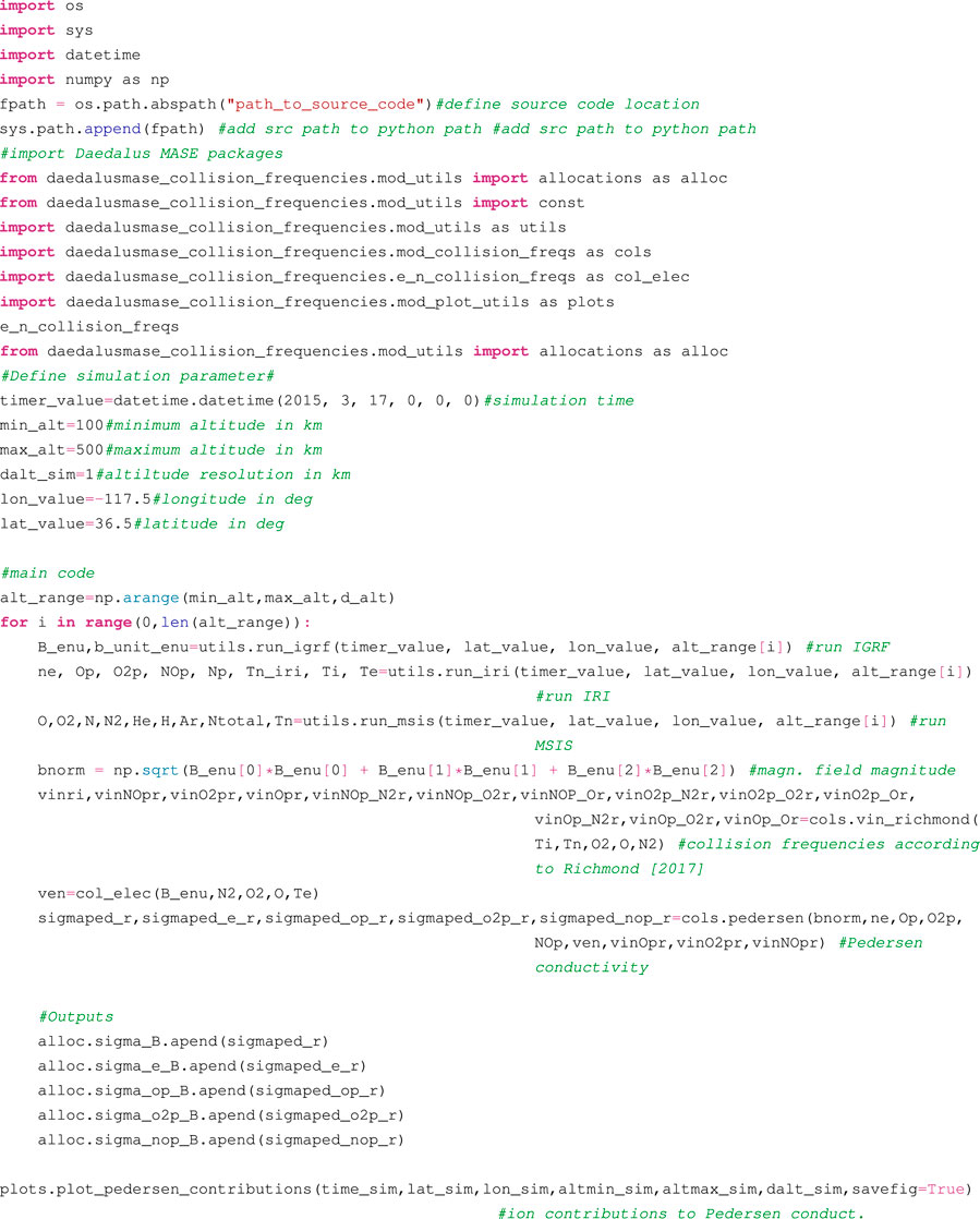
In order to import the modules, the user must follow the same procedure as described in Section 2.1.8 In the following, we present a code snippet which illustrates this procedure, along with the calculation of Pedersen conductivity. The output plot of this code is presented in Section 3.2, Figure 4A.

2.3 Error propagation module

As described above in Sections 2.1, 2.2, the calculation of the various derived products listed in Table 2 involves a long list of geophysical observables, or primary products, as listed in Table 1. For an in situ spacecraft or rocket borne mission, these primary observables are obtained through instruments with errors that can vary as a function of altitude, density, latitude, longitude, solar illumination conditions, spacecraft charging, etc. Thus, the resulting error of derived products is dependent on the errors of primary geophysical observables in a complex way. The aim of the module named daedalusmase_error_propagation is to enable the calculation of the relative contributions of errors of primary observables into the resulting error of a derived observable. Thus, after derived products are computed as discussed in Sections 2.1, 2.2, their uncertainties are estimated through standard propagation of variances through the respective analytical formulae. As errors are largely dependent on the instrumentation and the measurement methodology that is used, error estimates are introduced by the user per primary observable. As discussed in the Daedalus Report for Assessment (ESA, 2020), in the Phase-0 requirements definition study of Daedalus, assumed errors were introduced based on the corresponding targeted measurement uncertainty per observable. This enabled the cross-comparison of the effects that errors have in terms of their propagation into the resulting uncertainty in obtaining each of the derived observables.

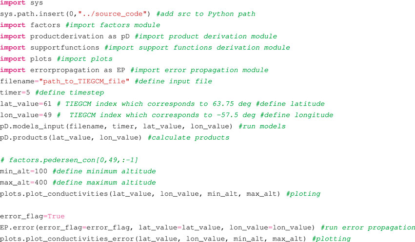
As an example, the three heating terms mentioned in Table 2 correspond to the same heating source, expressed in terms of different variables; similarly, two different methodologies were presented with respect to perpendicular current estimations. Thus, different corresponding instruments are used in their derivation, and the resulting errors are also expected to be different. The error propagation module enables the cross-comparison of the different estimation methodologies and their performance in terms of error in the various regions as a function of altitude and instrument characteristics (forward approach). Together with these heating terms, error propagation calculations were performed for all derived products listed in Table 2. Due to the multi-page extent of the formatted calculations of the resulting errors, the reader is referred to the Jupyter Notebooks that accompany the daedalusmase_error_propagation code. A list of the routines that comprise the module along with corresponding description is presented in Supplementary Table S9. We note that the errors introduced on the primary geophysical observables correspond to the total error, thus both random and systematic errors are injected. These are used to evaluate numerically the total errors propagating into the derived products. The values of the primary geophysical observables are obtained similarly to the modules described in Sections 2.1, 2.2 above, via GCMs. As an example call of the module, we present a code snippet for the calculation of the errors along altitude, over a specific latitude-longitude point:

2.4 Interpolation module

Physics based global circulation models such as TIEGCM, GITM and WACCM-X return results at a fixed number of locations, which most commonly are irregularly gridded. Hence a spatial interpolation scheme is needed to obtain an along-orbit estimate of any of the geophysical observables simulated in the GCM. In Daedalus MASE, an interpolation module named daedalusmase_interpolation is included as a standalone function and can be called by external programs as needed. The main program is written in python, however for large numbers of orbit points and large file sizes of the gridded datasets, interpolation can also be carried out by a subroutine written in C++, encapsulated in a python wrapper (F2PY3). The C++ subroutine adheres to the OpenMP interface, so the end user can opt for parallel interpolation. If opted for, the workload is distributed across as many processing threads as available, accelerating the execution. This is done as interpolating along orbit with a cadence of a few seconds through a gridded dataset consisting of thousands of points and for multi-year simulations is a computationally expensive process that requires parallel processing.

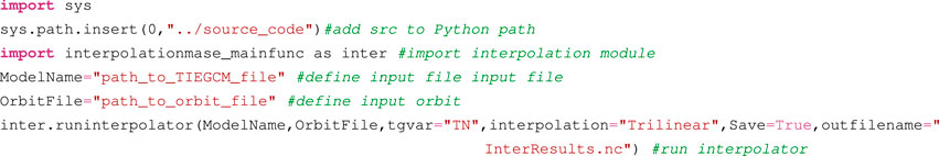
The method used in daedalusmase_interpolation is a trilinear interpolation scheme. A similar interpolation scheme was used by Elvidge et al. (2016) to interpolate data outputs from TIE-GCM and GITM to the position of the CHAMP spacecraft and then compare those with actual measurements. In daedalusmase_interpolation_scheme, the user can opt for first or second-order trilinear interpolation as well as other methods such as cubic splines. Given the orbit data of a specific mission, and depending on the method opted for, the interpolation scheme searches the 8, 16 or more neighboring grid points, deposits interpolating weights to each point and then interpolates those values to Daedalus’ position. When used in a multi-threaded environment the program can interpolate multiple positions in parallel. A list of the routines that comprise the module along with corresponding description is presented in Supplementary Tables S10. In the following, we present a code snippet for the trilinear interpolation of neutral temperature along a satellite orbit, through a TIEGCM NetCDF file:

2.5 Coverage calculation module

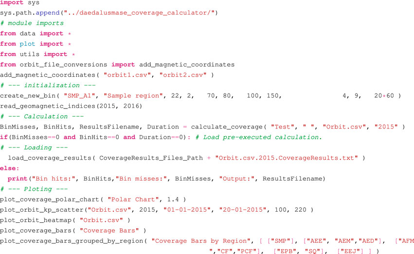
A key aim of the Daedalus mission assessment exercise is to demonstrate the ability of the proposed mission concept to capture geophysical observables and derived products related to the mission objectives globally with sufficient statistics. This module, named daedalusmase_coverage_calculator, aims to estimate the coverage of regions of interest with along-track measurements. The present module of Daedalus MASE allows introducing orbital files exported in standard formats from common orbital propagators, such as FreeFlyer (https://ai-solutions.com/freeflyer-astrodynamic-software/), NASA’s General Mission Analysis Tool (GMAT) (https://software.nasa.gov/software/GSC-17177-1)and Ansys Systems Tool Kit (STK) (https://www.ansys.com/products/missions/ansys-stk). Since key features in the ionosphere and thermosphere, such as electrical currents, auroral particle precipitation, plasma and neutral motion and magnetic disturbances are organized by the Earth’s magnetic field, magnetic coordinates are a more natural system in which to represent geophysical observables in the LTI (Laundal and Richmond, 2017); thus, module daedalusmase_coverage_calculator includes function AddMagneticCoordinates that appends magnetic latitude and magnetic local time information for each position along orbit. Subsequently, the user can enter details of the regions of interest, such as latitude (or magnetic latitude) and longitude (or magnetic local time) ranges by calling the function CreateNewBin.

Based on these ranges, this module then performs estimates of the coverage in terms of total sampling time within these regions of interest over the mission lifetime. The module also enables estimating the total sampling time under user-defined conditions, such as solar illumination and the Kp index of geomagnetic activity. The calculations are executed by function calculate_coverage and the results are saved in a file. Prior to the calculation, the user can set the paths of the files by calling functions set_orbit_files_path, set_coverage_results_files_path, and set_geomagnetic_indices_files_path. The user must also call function read_geomagnetic_indices to specify the time period of interest.

The resulting data produced by the above calculations can be used directly to create charts. Past coverage calculations can be retrieved by calling function load_coverage_results. Charts can be created by functions plot_coverage_bars, plot_coverage_bars_grouped_by_region, plot_coverage_polar_chart, and plot_orbit_kp_scatter, plot_orbit_heatmap.

A list of the routines that comprise the module along with corresponding description is presented in Supplementary Table S11.

As an example, the following function presents the use of the daedalusmase_coverage_calculator module.

2.6 Global statistics module

A key question that often accompanies in situ sampling schemes is whether a specified orbital scenario will obtain, over the mission lifetime, statistically representative measurements within the regions of interest. For example, as part of its primary science objectives, Daedalus aims to quantify Joule heating (among other derived products) within the regions where it maximizes; thus, a key requirement of the Daedalus mission is for Joule heating to be estimated globally with sufficient statistics, so that the in situ measurements are representative of the variability of Joule heating and can enable reproducible parameterizations of Joule heating in global models. The related performance metrics of the Daedalus mission set the thresholds of when a statistically representative coverage can be obtained over the mission lifetime, which was defined in terms of the mean and variance of Joule heating within the identified regions of interest. The purpose of this module, named daedalusmase_global_statistics, is to investigate quantitativelywhether the dataset of a variable obtained via an in situ sampling scheme is sufficiently large and diverse to determine the average value of both primary geophysical observables, such as those presented in Table 1, and derived products, such as those of Table 2, within each region of interest, to within a specified fraction of the median (as determined from models), and for a specified range of driving conditions. In the Daedalus mission performance simulations, using the Daedalus MASE code, this was demonstrated via the following scheme:

1. TIEGCM was run for the minimum mission lifetime of Daedalus, corresponding to a 3 year lifetime, with a temporal resolution corresponding to approximately the orbital period.

2. The gridded dataset of TIEGCM was sampled along orbit via an interpolation scheme (see module daedalusmase_interpolation_scheme described above).

3. Regions of interest (or bins) were defined by ranges of altitude, magnetic latitude, magnetic local time and the Kp index of geomagnetic activity.

4. Statistics were assembled within the regions of interest, and the mean and variance were calculated within the pre-set bins.

5. The statistical characteristics of the dataset of the along-orbit sampling of TIEGCM were compared to the characteristics of the dataset that included the full statistics of all TIEGCM gridded points within the regions of interest. Accordingly, a statistical distribution or Probability Density Function (PDF) of Joule heating was constructed for each of the defined regions of interest based on Joule heating measurements along the orbit, and the PDF was compared with the corresponding PDF from the full statistics of TIEGCM gridded points. For the comparison, the median value (Me) and Median Absolute Deviation (MADe) were calculated and inter-compared.

6. The statistical significance of the along-orbit sampling when compared to truth was evaluated by performing the Wilcoxon Rank Sum Test for the two PDFs. This metric gives an estimate of what constitutes a statistically significant sample of measurement locations so as to enable the accurate parameterization of derived products.

The result of the above module was to provide a metric that allows estimating what constitutes a statistically significant sample of measurement locations so as to enable the accurate parameterization of the sampled primary and derived products. The sample of measurement locations, termed mission coverage performance, enables quantifying the sampling requirements of the mission and justifying the orbit selection. The mission sampling requirements thus evolve iteratively in concert with mission performance assessments in Daedlus MASE, chosen to ensure globally adequate statistical representation of the main derived products within predefined regions.

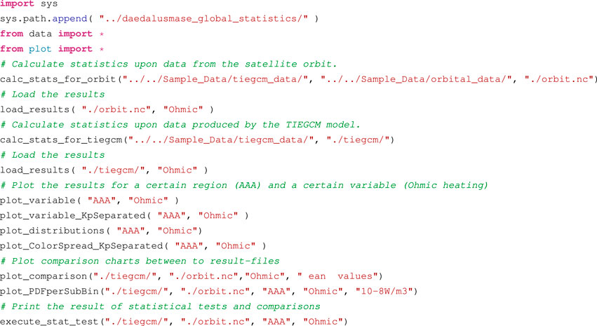
The calculation of the statistics per region of interest is performed by the function calc_stats_for_orbit for along-orbit sampling of TIEGCM and by the function calc_stats_for_tiegcm for the ensemble of the TIEGCM gridded points. The results are separated by user-specified regions of interest and are saved in files of NetCDF format. These data can be subsequently read by the function load_results and plotted by the functions plot_variable, plot_variable_KpSeparated, plot_distributions and plot_ColorSpread_KpSeparated. The user can also call plot_comparison, plot_PDFperSubBin and execute_stat_test in order to directly compare along-orbit statistics with global-TIEGCM statistics.

A list of the routines that comprise the module along with corresponding description is presented in Supplementary Table S12.

The following example shows the calculation of statistics based on data from a sample satellite orbit. Statistics are calculated based on gridded data produced by the TIEGCM model.

2.7 3D visualizations module

In order to demonstrate the nature of Daedalus in situ measurements, to clarify the mission’s orbit geometry, and to provide global context to the measurements based on model output, a set of graphics and 3D visualizations were produced during the course of the Daedalus Phase-0 study. The scope of this section is to describe the process and present the code that results in a number of high-quality graphics and visualizations that can be produced based on GCM outputs.

The 3D visualizations involve the following steps:

1. Global model outputs of the thermosphere-ionosphere are produced using GCMs. The output data consist of NetCDF files.

2. Based on simulated orbit ephemeris data, observations from an in situ mission are simulated along orbit, utilizing the interpolation module, as described above.

3. Interfaces are created between the input data sources and graphics software, including Generic Mapping Tools https://doi.org/10.1029/2019GC008515 for 2D graphs and text annotations and Blender https://www.blender.org for 3D rendering. The interface to Generic Mapping Tools has been created using the relatively new Python interface, PyGMT (https://doi.org/10.5281/ZENODO.4522136), which allows direct integration of GMT commands in a Python script or Jupyter notebook.

4. The visualisation is set up using the graphics software, and visual exploration of the data and models is initiated, resulting in a selection of (motion) graphics output.

5. The 3D graphics and motion graphics are edited in software such as Adobe Illustrator for static 2D graphics and Apple Motion for animations. In particular, the Motion software makes it easy to combine (composite) many 2D and 3D elements in a single animation, such as the 2D date/time annotations, AE-index graph and colour bars (created with Generic Mapping Tools) with the three separately 3D-rendered Earth and atmosphere model outputs (created with Blender) in 9.

6. Figures and animations are subsequently exported in high resolution formats. Examples of the animations can be found via the links in the presentation by Doornbos et al. (2020) as well as in the website: https://daedalus.earth.

It is noted that, for interfacing with Blender, two methods were explored. At first, Python scripts and Jupyter notebooks were used to create files outside of Blender, in formats that can be imported by a user via the standard Blender graphical user interface. These file formats include Wavefront Object files (.obj) for static geometry, Point Cache (.pc2) files for time-varying geometry, and PNG graphics for textures to be used on the 3D geometry. This approach required extensive overhead in terms of file management and setting up of scenes inside of Blender. A second approach that was explored was to integrate this code with Blender’s Python API, effectively creating a plug-in for Blender in which collections of NetCDF model output files and satellite orbit parameters can be selected for rendering. In principle, this approach could lead to an easily reusable plugin package, however, open issues with the installation of the plug-in and Python package dependencies currently still prohibit easy adoption.

The resulting output of the 3D visualizations scheme consist of high-quality graphics in terms of content, style and resolution, as well as scientific figures and animations for a variety of audiences and for explaining and promoting the science and physics processes of the LTI. These visualizations enable to provide feedback, based on the visual exploration of the models and simulated data, on aspects related to the underlying physics of the processes explored, to the sampling characteristics, to the data processing approaches, etc. The aim of the present section and the dissemination of the code that produces these 3D graphics and visualizations is to support other scientists in producing high-quality and clear graphics of GCM outputs.

3 Results

In the following, we present some sample results from running the above modules of DaedalusMASE. These are not comprehensive and are only meant to be used as examples for using these modules, demonstrating some of their capabilities; the user is referred to the corresponding code and related online documentation for more information and for an outline of their full capabilities.

3.1 Sample results from daedalusMASE_derived_products

Using the daedalusmase_derived_products Jupyter notebook, the user can select to calculate various derived products as well as plot both primary and derived products in GCM simulation outputs. This module currently reads NetCDF files as formatted through standard TIEGCM simulation outputs, but can be easily adapted to use outputs from GITM, WACCM-X and other GCMs that provide a comprehensive list of LTI variables. Through a Graphical User Interface as shown in Figure 2, the user can select the TIEGCM input file, the pressure level and the timestep, and the desired parameters to be plotted. Also, one can select from a list of different maps to plot the results. Moreover, an orbit and nightshade can be added to the plots.

FIGURE 2

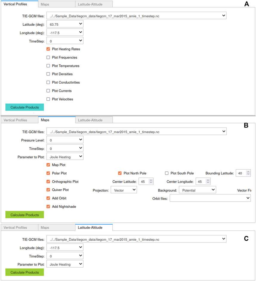
FIGURE 2. Graphical User Interface (GUI) for calculating and plotting: (A) vertical (altitude) profiles of various primary and derived products in TIEGCM; (B) derived products in TIEGCM as a function of latitude-longitude maps; and (C) latitude-altitude profiles of derived products in TIEGCM.

The comprehensive list of scalar products (both primary and derived) that can be calculated and/or plotted from this module includes: 1) Joule, Ohmic and frictional heating, 2) Convection heating and wind correction term, 3) Ohmic heating per unit mass and ratio of Joule heating over pressure, 4) Heat transfer to the neutral gas, 5) Pedersen, Hall and total perpendicular conductivities, 6) Ion neutral collision frequencies and Ion neutral cross sections.

The comprehensive list of vector products (both primary and derived) that can be calculated and/or plotted from this module includes: 1) Pedersen, Hall and total perpendicular currents, 2) Magnetic forcing vector, 3) Electric Field, 4) Magnetic Field, 5) Ion drifts, 6) Neutral winds.

It is noted that Daedalus MASE offers the possibility to plot altitude profiles for specific cases and over specific times and locations. These can be of use for multiple applications, including for ground-based investigations that utilize collision frequency models or rocket flights that do not incorporate neutral density measurements.

In Figure 3 we present some examples of different formats for plotting the scalar and vector products: In Figure 3A we plot Joule heating rate in mW/m³ in 2D latitude-longitude plot. In Figure 3B we present an altitude-latitude cut of Joule heating. A northern polar plot of the Pedersen conductivity is shown in Figure 3C. In Figure 3D a streamline plot of electric field plotted over a polar plot of the electric potential is shown. Lastly, in Figure 3E, an orthographic view of the global Joule heating rate distribution is presented.

FIGURE 3

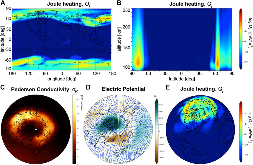
FIGURE 3. (A) 2D latitude-longitude map of Joule heating rate at 120 km. (B) Altitude-latitude plot of Joule heating rate along a meridional cut at fixed longitude. (C) Polar plot (north) of Pedersen Conductivity at 120 km, (D) Polar plot (north) of electric potential with overlaid streamlines of electric field, at 120 km. (E) Orthographic global plot of Joule heating at 120 km. All plots correspond to the peak of St. Patrick’s day storm, 17 March 2015, 13:55 UT.

3.2 Sample results from daedalusMASE_collision_frequencies

In calculations of the Pedersen conductivity, σ_P, the ratio (κ_i) of each species’ gyrofrequency versus its collision frequency needs to be estimated. The collision frequency depends, in turn, on the species’ density, thus neutral composition needs to be known. The variability of conductivities stems mainly from the variability of electron density N_e, of the neutral density N_n of various n species, from the temperature-dependent ion-neutral collision frequencies, ν_in, and, to a lesser extent, the magnetic field strength B, which remains rather constant with altitude and is well known in the limited range of LTI altitudes, at least compared to other geophysical observables. The above enter the equations for all three conductivities described in Section 2.1.2 (Eqs 20–22), namely, σ_P, σ_H, and σ_‖. To investigate the variability of collision frequencies between the different models, and further to demonstrate the effect that such a variability of collision frequencies has on conductivities, and, through that, on Joule heating and currents, in Figure 4 we plot: a) the contribution of electron and ion species to the Pedersen conductivity b) normalized collision frequencies of O⁺−O (i.e., collision frequencies divided by the O density) as a function of altitude, based on the various approximations or models, as marked; c) altitude profiles of the ion-neutral collision frequencies, as obtained for the conditions of St. Patrick’s day 2015 storm; and c) altitude profiles of Pedersen conductivities, calculated according to the different ν_in of panel d). The impact of the different ν_in models in the calculation of the Pedersen conductivity is evident in the F region (200–300 km) where significant discrepancies can be observed in σ_P.

FIGURE 4

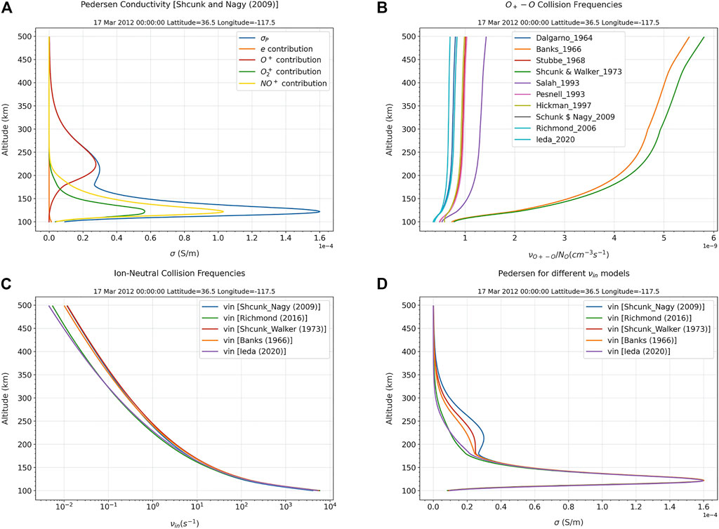
FIGURE 4. (A) Electron and ion contributions to the Pedersen conductivity (B) Normalized collision frequencies of O⁺−O as a function of altitude, based on the various models, as marked; (C) altitude profiles of the ν_in collision frequencies during St. Patrick’s day 2015 storm; and (D) altitude profiles of the Pedersen conductivity, calculated with ν_in from different models as marked.

3.3 Sample results from daedalusMASE_error_propagation

Using the Daedalus MASE error propagation calculations module, the user can select to calculate the error propagated onto various derived products, as listed in Table 2, as well as plot errors as a function of altitude or as maps in latitude and longitude. Through a Graphical User Interface as shown in the Figure 5A, the user can select the TIEGCM input file, the errors per geophysical observable, and the desired parameters for which to calculate the propagated error.

FIGURE 5

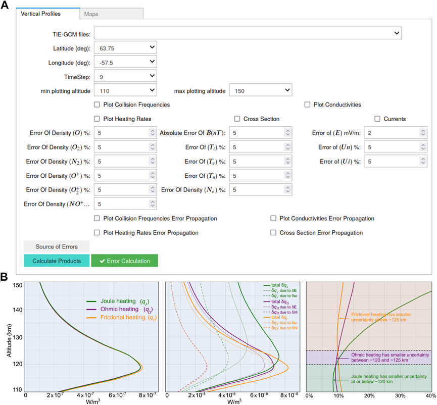
FIGURE 5. (A): a Graphical user Interface (GUI) for the selection of parameters of the error propagation, such as the location, derived product and errors per geophysical observables. (B): Example of Joule heating total uncertainty propagation for a vertical profile at 63.75^o latitude, −57.5^o longitude, 2015-03-17 18:00, for the three estimation methods. Left, profiles as drawn from TIEGCM grid column. Middle, absolute total uncertainties, and principal contributors to total uncertainty (electric field δ E, ion drift δ vi, and ion number density δ Ni). Right, relative total uncertainties in E region.

As an example of the propagation of errors in the calculation of derived products, in the Figure 5B we show the inter-comparison of the errors in obtaining Joule, Ohmic and frictional heating, the three different estimates of the same process by which the relative motion of plasma and neutrals results in heating in the LTI. The total uncertainty propagated onto the corresponding heating profiles, based on assumed uncertainties on the contributing (primary) variables, is shown in this figure as a function of altitude. The vertical profiles are obtained during the peak of a geomagnetic storm that occurred on 17 March 2015, also referred to as St Patrick’s day storm 2015. This figure illustrates how the three estimates produce very similar profiles–at least in the self-consistent model world–and how the uncertainty of the methods is predicted to differ, as a function of altitude. Here, it is shown that the relative total uncertainty of at least one of the methods stays well below 15% throughout the E region.

The individual errors of the various geophysical observables that were introduced in the above exercise are consistent with the observational requirements in terms of total errors; however, this module allows realistic or actual measurement errors to be introduced in a similar fashion. Furthermore, errors can be injected in this module after being estimated through parametric instrument simulators. Errors can thus be a function of the local environment, such as altitude, solar illumination, latitude, etc. In particular, the low altitudes of the LTI are known to introduce wake effects and ram perturbations to various geophysical observables; this module enables injecting estimated errors of measured quantities and propagating their effects onto the derived products.

3.4 Sample results from daedalusMASE_interpolation_scheme

In the following we present an example of the along-track interpolation, at 10-s intervals, which is used to produce synthetic time series data from GCM gridded datasets. In the case of the Daedalus Mission Assessment exercise, the interpolation of the GCM gridded dataset enabled the creation of synthetic geophysical observable time series, which were extracted along realistic orbit tracks. The data underpinning this exercise consisted of a mission lifetime global self-consistent simulation of the comprehensive LTI environment, which corresponded to 3 years; this simulation was then sampled along a 3-year set of simulated orbits, producing the synthetic time series.

The left-hand side of Figure 6 shows an example of an orbit of the Daedalus spacecraft, with vectors of the neutral winds, ion drifts and electron drifts over-plotted along the orbit. The middle panels show a “dashboard” of instantaneous measurements, obtained through the along-orbit interpolation. The right-hand side panels show, in sequence from top to bottom, the geodetic latitude, longitude and altitude of the simulated spacecraft orbit, and the along-orbit interpolated time series of electron density. Further to the application for the Daedalus Mission Performance Demonstrations, the creation of synthetic time series enables the cross-comparison of model data with measurements from satellites, as well as the creation of model altitude profiles for ground-based investigations that utilize collision frequency models or rocket flights.

FIGURE 6

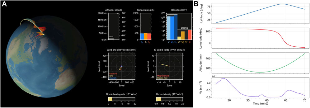
FIGURE 6. Example of the along-orbit interpolation of various primary geophysical observables: The (A) (globe) shows sample orbit of Daedalus, with vectors of neutral winds and ion drifts plotted along the orbit; the middle panels show a “dashboard” of instantaneous measurements, obtained through the along-orbit interpolation; the (B) show spacecraft latitude, longitude, altitude, and along-orbit time series of electron density.

3.5 Sample results from daedalusMASE_coverage_calculator

In support of the scene generation and performance demonstration modeling, Daedalus lifetime simulations were performed using TIEGCM, for the baseline duration of the Daedalus mission (3-year), with the following considerations: The time period for the 3-year TIEGCM scene generation runs was selected based on the phase of the solar cycle expected during the launch of Earth Explorer 10, originally planned for 2027 or 2028. Since geomagnetic activity is largely solar cycle-driven, the corresponding phase of the past solar cycle was simulated. The consensus prediction for the timing of the next solar cycle (solar cycle 25) is given in Figure 7, based on solar sunspot number prediction. It was thus expected that Daedalus’ launch would occur during the descending phase of the solar cycle. The most recent descending phase was that of solar cycle 24, also shaded in the Figure 7A. The corresponding time period is from 1 January 2015, until 31 December 2017.

FIGURE 7

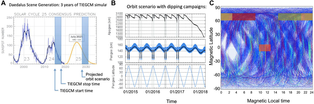
FIGURE 7. (A): Historical record of solar cycles 23 and 24, and consensus prediction of solar cycle 25. (B): Orbital parameters based on simulations of a sample Daedalus orbital scheme. (C): Latitude vs local time coverage in the 100–200 km altitude range; color-coded is the Kp index, ranging from 0 (in blue) to 9 (in red).

Subsequently, an orbital simulation was run, based on atmospheric drag predictions for the same time period. The orbital simulation includes apogee maintenance and perigee descent maneuvers to lower-most altitudes from nominal altitudes, aiming to address the coverage requirements, as stated in ESA. (2020). A summary of orbital information based on the orbital design of the Daedalus Mission Concept is given in the Figure 7B, according to Sarris et al. (2020). An example of orbital tracks is shown in the Figure 7C, where the Kp index is plotted in color along Daedalus’ orbit. Regions of interest are marked in colored rectangular stripes, and within these regions statistics of the obtained measurements are calculated using module daedalusmase_global_statistics.

3.6 Sample results from daedalusMASE_global_statistics

Based on the calculation of the derived products, as described Sections 3.1, 3.2, and the coverage calculations, as described in Section 3.5, the purpose of this module is to estimate the statistical significance of obtaining various primary and derived products with the along-sampling scheme of in situ measurements by the Daedalus mission concept.

Figure 8 demonstrates the comparison between the statistical distribution of Joule heating as calculated by the TIEGCM model, shown in the top panels, and Joule heating as sampled in situ along the orbit with a cadence of 1 s, as shown in the lower panels. An altitude profile of Joule heating is shown in the left panels, were the region of interest that is investigated is the auroral midnight sector, defined by Magnetic Latitudes of 60–75°, Magnetic Local Time between 21:00 and 03:00 and Altitude of 100–160 km. Ohmic heating as a function of magnetic latitude and local time is shown in the right panels. The lower panels visualize the accuracy to which each region can be described by the orbit samples.

FIGURE 8

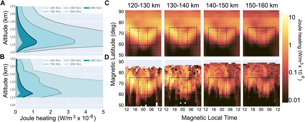
FIGURE 8. (A,B): Statistical distribution of Joule heating in altitude, as calculated by all gridded data of TIEGCM within magnetic latitudes from 60 to 75° and local time between 21:00 and 03:00 (A) and as sampled along orbit within the same region (B). (C,D): Statistical distribution of Joule heating in magnetic latitude and local time, for four altitude bins, as marked, based on all TIEGCM gridded data (C) and along-track sampling (D).

Further to the visual inter-comparison shown in Figure 8, as described in Section 2.6, in order to evaluate the statistical significance of the along-orbit sampling when compared to truth (i.e., the gridded dataset), this module calculates the median values (Me) and Median Absolute Deviation (MADe) for the two datasets, and also performs the Wilcoxon Rank Sum Test for the two PDFs.

3.7 Sample results from daedalusMASE_3D_visualizations

In Figure 9, as an example of 3D visualizations, a snapshot of the evolution of key geophysical observables in the LTI are given: temperature, electron density and neutral winds are plotted as a function of pressure level in the Thermosphere during a geomagnetic storm event, as parameterized here via the auroral electrojet (AE) index of geomagnetic activity, following a fast-moving Coronal Mass Ejection (CME) that hit the Earth’s magnetic field. The AE index, shown in the lower center part of Figure 9, provides a global, quantitative measure of auroral zone magnetic activity produced by enhanced ionospheric currents flowing below (i.e., at sub-auroral latitudes) and within the auroral oval; the red line indicates the snapshot time. As it can be seen in the movie of this event in the Supplementary Material, initially, solar EUV radiation dominates, causing diurnal variations. Later on in the simulation, intense variations are observed, primarily at high latitudes, causing travelling disturbances that move to lower latitudes, as well as longitude-dependent variability. These effects are caused by energetic particle precipitation (EPP) from the magnetosphere into the atmosphere, together with waves, tides and gravity waves from below and also by Joule heating (JH) of the lower thermosphere due to mega-Ampere currents that are closing within the same 100–200 km range where temperature and composition change drastically.

FIGURE 9

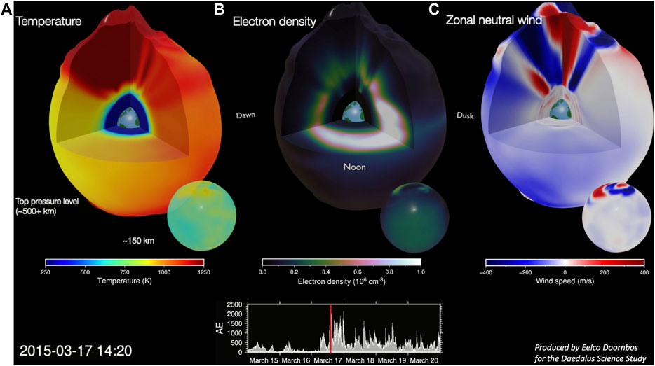
FIGURE 9. 3D visualization of GCM model outputs: neutral temperature (A), electron density (B) and zonal neutral wind (C). The model output is from the 2015 St. Patrick’s Day storm, showing the simulated state of the atmosphere on 17 March 2015, 14:20 UTC, during a period of significant forcing from above. Pressure level geopotential heights from the model have been exaggerated by 50 times to show vertical detail. Small spheres at the lower right side of each large sphere show the corresponding values at altitudes ∼150 km.

4 Summary and conclusion

Daedalus MASE routines and modules were originally designed as a mission simulator for the Daedalus mission concept, which targets to sample the LTI with in situ measurements down to extreme low altitudes, with a main focus in the under-sampled altitude range of 100–200 km. The underlying assumption for Daedalus MASE is that the primary observables used for the calculation of derived quantities are obtained by instruments capable of performing measurements in situ, and the goals of the mission simulator included the assessment of the closure of the mission objectives by the in situ sampling scheme of Daedalus, including, but not limited to, the demonstration of achieving the calculation of a set of derived products, an assessment of the errors that propagate onto these derived products, estimates of the coverage times from an in situ sampling scheme, and an assessment of the statistical significance of the in situ sampling scheme. However, beyond their initial usage as a mission simulator for the Daedalus mission, the modules comprising Daedalus MASE have evolved to include a number of tools that can be used for performing various scientific analyses of in situ spacecraft measurements of various observables, for processing and plotting gridded model datasets of Global Circulation Models of the Earth’s thermosphere and ionosphere, and for performing comparisons between satellite data and models.

As an example, the Electric Field Instrument (EFI) onboard the Swarm satellites (Knudsen et al., 2017), which fly on near-polar, circular orbits with altitudes that range from 400 to 530 km, perform measurements of plasma densities and electron temperatures, both of which are also outputs of TIEGCM. By interpolating the TIEGCM gridded dataset along the Swarm orbits, the two time series can be inter-compared for similarities and for differences: the former allow using the larger picture, as captured by TIEGCM, to interpet the along-track observations, whereas the latter enable identifying missing physics and small-scale, sub-grid variability in the models. Similarly, neutral density data from the Swarm accelerometers (Siemes et al., 2016) as well as from Swarm GPS observations (van den Ijssel et al., 2020) can also be cross-compared with model data using Daedalus MASE. Furthermore, Daedalus MASE tools allow performing comparisons of statistical values as obtained from TIEGCM with the statistical ensemble of along-orbit data, such as those made by Swarm, gathered over longer time periods that enable classifications in areas of interest and as a function of geomagnetic conditions.

Similarly, the Ionospheric Connection Explorer (ICON) mission, which flies in a circular, low-inclination orbit at an altitude of 575 km, retrieves, among other parameters, in situ vertical ion drifts, the peak of ionospheric density, and altitude profiles of neutral temperature, wind vectors and densities of O and N₂. All the above quantities are output geophysical observables in TIEGCM, and Daedalus MASE allows their extraction and plotting, either along-track or as altitude profiles from TIEGCM, enabling their direct comparison. We note in particular the recent development of TIEGCM-ICON, driven by tidal perturbations derived from ICON observations and at high latitude by ion convection and auroral particle precipitation patterns from AMIE, the Assimilative Mapping of Ionospheric Electrodynamics model (Maute, 2017); Daedalus MASE routines are directly applicable to TIEGCM-ICON as well, assisting in comparative studies between ICON observations and TIEGCM-ICON model outputs. As further enhancements of Daedalus MASE, special pre-set routine settings can be devised that enable the extraction of, e.g., altitude profiles in the altitude ranges and vertical resolutions as described in the Level 2 data descriptions of ICON. In addition, the use of the modules described in Sections 2.5, 2.6 enables the calculation of statistical properties of long-term time series and the estimation of their statistical significance in user-defined bins in terms of local time, latitude and geomagnetic activity.

In terms of processing of the outputs of GCMs (gridded datasets), potential scientific analyses enabled by Daedalus MASE include the calculation of various derived products based on geophysical quantities (or primary products) of GCMs on all grid-points of the GCM simulation, the production of maps, altitude profiles and latitude–local time cuts in GCMs, the conversion of geographic gridded points to magnetic coordinates, height integrations, and calculations of globally or hemispherically integrated quantities.

It is noted that the derived products calculated via Daedalus MASE are of prime interest in the E region and lower F region, as they relate to key unknown properties in these regions (see, e.g., Sarris. (2019); Palmroth et al. (2021)). It is also noted, however, that many of these quantities are not directly calculated in GCMs. Thus Daedalus MASE fills a gap by providing a comprehensive toolset for the direct calculation of each of these quantities. These can be readily integrated with existing codes, can be expanded to perform additional calculations and cross-comparisons, or can be used as a stand-alone toolset for the post-processing of GCM datasets, including plotting of GCM snapshots and movies in various forms, through 2D and 3D global maps and various altitude/latitude/longitude cuts.

The calculation of these derived products is accompanied by error propagation estimation routines, for the inclusion of measurement errors; errors can also be obtained through simplified parametric instrument simulators, or through analytic (e.g., altitude- or density-dependent) error models. Subsequently, derived products are computed, and their uncertainties are estimated through standard propagation of variance for the respective analytical formulae. Data from the solar cycle run of TIEGCM are available upon request (see data availability statement below).

These functionalities are potentially useful to the broader space physics community that use GCM outputs for LTI science. Applications are presented focusing on gridded datasets produced by NCAR’s TIEGCM, however, the analysis tools of Daedalus MASE can be expanded to be applicable to other gridded geophysical observable data, that can be obtained from, e.g., the Whole Atmosphere Community Climate Model with thermosphere and ionosphere extension (WACCM-X), or the Global Ionosphere Thermosphere Model (GITM).

Further to the modules described herein, which enable various computations based on the gridded datasets, Daedalus MASE also includes additional code and modules that are specific to the Daedalus mission, and which are not described herein. These include, for example: an instrument-specific module for the calculation of the electric field that enables calculating the effect of spacecraft velocity on the resulting electric field and its dependence on the boom length; code enabling the reconstruction of pitch angle distributions of energetic particles based on a fixed number of particle detectors; simulations of the effect of energetic particles on the lower atmosphere. Furthermore, Vogt et al. (2022) expanded upon earlier work on the altitude reconstruction of primary and derived products based on multi-point measurements, addressing the question of how in situ measurements in the LTI can be extrapolated using parametric models of observables and derived variables: Using ensembles of model parameters, created by means of Monte Carlo simulations and synthetic measurements based on model predictions and relative uncertainties, they presented a methodology that allows for assessing how cost-critical elements of the Daedalus mission such as perigee and apogee distances affect the accuracy of the reconstruction of various ionospheric profiles.

The modules for the calculation of various derived products in Daedalus MASE are accompanied by Jupyter Notebooks that include the equations and code calculating these derived products, together with literature references. Most importantly, these Jupyter Notebooks include easy-to-use plotting functions, enabling 2D and 3D plotting on maps, altitude profiles and various user-defined cuts, enabling the quick processing and useability of GCM outputs. This is combined with having all relevant code in python, thus enabling the user to build upon the existing framework. Daedalus MASE also includes interpolation routines that can estimate primary and derived products at any location within a gridded dataset. This includes points along spacecraft and rocket orbits, altitude profiles, ground instrument lines of sight, etc.

Combining the above functionalities, together with derived product calculations and uncertainty estimations, Daedalus MASE enables performing coverage simulations for various assumed mission lifetimes and orbit options, in order to determine and demonstrate the statistical significance of the data collected and of representing global processes in the LTI via in situ measurements. This is of particular importance for a low-altitude mission such as Daedalus, where sampling the lowermost altitudes has significant implications for the mission duration, required propulsion and, overall, mission complexity, due to enhanced atmospheric drag. Thus, besides the proposed mission concept Daedalus, direct application of Daedalus MASE can be made for other in situ sampling schemes, such as the upcoming Geospace Dynamics Constellation (GDC), a mission concept that targets to study the coupling between the magnetosphere and the ionosphere/thermosphere (IT) system, and how that coupled system responds to external energy input. Daedalus MASE tools can also be applied to rocket measurements: even though rockets often lack the comprehensive ensemble of all relevant instruments to measure ion-neutral interactions, Daedalus MASE allows substituting a measurement by modeled along-flight parameters, while also enabling sensitivity analyses of the effects of model and measurement errors on the calculated parameters.

Data availability statement

The datasets and source code presented in this study can be found in the following online repositories: The source code of the Daedalus MASE modules described in this study as well as sample datasets of TIEGCM outputs, geomagnetic indices and sample orbit files, can be downloaded from the Daedalus MASE repository, at link: https://github.com/DaedalusMASE/DaedalusMASE. The source code for the 3D visualizations of GCM outputs can be downloaded at: https://gitlab.com/eelcodoornbos/blender_gcm_slices. The names of the modules and subroutines in the above repositories can be found in the article/Supplementary Material.

Author contributions

TS coordinated the study and wrote the first draft. ST wrote Sections 2.1, 2.2, 3.1, 3.2 and corresponding code. PP wrote Sections 2.3, 3.3 and corresponding code. CHP contributed to the code discussed in Sections 2.1 and 3.1. PP and KP wrote Sections 2.4, 3.4 and corresponding code. DB wrote Sections 2.5, 2.6, 3.5, 3.6 and corresponding code. ED wrote the code described in Sections 2.7, 3.7. TS, SB, ED, MC, ID, WM, DK, NO, OM, TOM, AM, MP, CS, NI, RP, TM-J, CS contributed to the conception and design of DaedalusMASE functionality as members of the Daedalus Mission Advisory Group. AH, DL, AS, MT contributed to the conception and design of Daedalus MASE functionality as ESA technical officers overlooking the Daedalus Science and Requirements Consolidation study. MC, PV, DM, NA, AK, WM, JV, AB, NS contributed to other parts of DaedalusMASE code, not described herein, and expanded upon functionality of DaedalusMASE. H-LL, GL, ST contributed to the TIEGCM model runs and model data collection. IS and COP contributed to the independent review and testing of the code. All authors contributed to the scientific analysis. All authors contributed to manuscript revision and approved the submitted version.

Funding

Funding for the development of the modules in DaedalusMASE was provided by the European Space Agency under contract number 4000127346 to the Democritus University of Thrace (study title: Daedalus Phase-0 Science and Requirements Consolidation Study). The research work by TS was supported by DUTH project KE82875. The research work by ST was supported by the Hellenic Foundation for Research and Innovation (HFRI) under the HFRI PhD Fellowship grant (Fellowship Number: 400), and DUTH project KE82372.

Acknowledgments

Daedalus MASE was developed during the Phase 0 study of Daedalus, one of three candidate mission concepts for ESA’s 10th Earth Explorer.

Conflict of interest

Authors IS and CP were employed by the company Space Applications Research Consultancy.

The remaining authors declare that the research was conducted in the absence of any commercial or financial relationships that could be construed as a potential conflict of interest.

Publisher’s note

All claims expressed in this article are solely those of the authors and do not necessarily represent those of their affiliated organizations, or those of the publisher, the editors and the reviewers. Any product that may be evaluated in this article, or claim that may be made by its manufacturer, is not guaranteed or endorsed by the publisher.

Supplementary material

The Supplementary Material for this article can be found online at: https://www.frontiersin.org/articles/10.3389/fspas.2022.1048318/full#supplementary-material

References

Archer, W. E., Knudsen, D., Burchill, J., Jackel, B., Donovan, E., Connors, M., et al. (2017). Birkeland current boundary flows. J. Geophys. Res. Space Phys. 122, 4617–4627. doi:10.1002/2016ja023789

CrossRef Full Text | Google Scholar

Banks, P. (1966). Collision frequencies and energy transfer electrons. Planet. Space Sci. 14, 1085–1103. doi:10.1016/0032-0633(66)90024-9

CrossRef Full Text | Google Scholar

Banks, P. M., and Kockarts, G. (1973). Aeronomy. New York, NY: Academic Press.

Google Scholar

Bilitza, D. (2018). Iri the international standard for the ionosphere. Adv. Radio Sci. 16, 1–11. doi:10.5194/ars-16-1-2018

CrossRef Full Text | Google Scholar

Billett, D., Grocott, A., Wild, J., Walach, M.-T., and Kosch, M. (2018). Diurnal variations in global joule heating morphology and magnitude due to neutral winds. J. Geophys. Res. Space Phys. 123, 2398–2411. doi:10.1002/2017ja025141

CrossRef Full Text | Google Scholar

Cowley, S. (2000). Magnetosphere-ionosphere interactions: A tutorial review. Magnetos. Curr. Syst. Geophys. Monogr. Ser. 118, 91–106. doi:10.1029/GM118p0091

CrossRef Full Text | Google Scholar

Crisp, N. H., Roberts, P. C., Livadiotti, S., Oiko, V. T. A., Edmondson, S., Haigh, S., et al. (2020). The benefits of very low Earth orbit for Earth observation missions. Prog. Aerosp. Sci. 117, 100619. doi:10.1016/j.paerosci.2020.100619

CrossRef Full Text | Google Scholar

Dalgarno, A., Henry, R., and Stewart, A. (1964). The photoionization of atomic oxygen. Planet. Space Sci. 12, 235–246. doi:10.1016/0032-0633(64)90225-9

CrossRef Full Text | Google Scholar

Deng, Y., Maute, A., Richmond, A. D., and Roble, R. G. (2009). Impact of electric field variability on joule heating and thermospheric temperature and density. Geophys. Res. Lett. 36, L08105. doi:10.1029/2008gl036916

CrossRef Full Text | Google Scholar

Deng, Y., and Ridley, A. J. (2007). Possible reasons for underestimating joule heating in global models: E field variability, spatial resolution, and vertical velocity. J. Geophys. Res. 112, 12006. doi:10.1029/2006ja012006

CrossRef Full Text | Google Scholar

Doornbos, E., Sarris, T., Tourgaidis, S., Pirnaris, P., Buchert, S., Liu, H., et al. (2020). “Visualizing models and observations of the thermosphere-ionosphere in support of the ESA EE10 candidate mission Daedalus,” in EGU general assembly 2020 (Vienna: European Geophysical Union), 7386. doi:10.5194/egusphere-egu2020-7386

CrossRef Full Text | Google Scholar

Drob, D., Emmert, J., Crowley, G., Picone, J., Shepherd, G., Skinner, W., et al. (2008). An empirical model of the Earth’s horizontal wind fields: HWM07. J. Geophys. Res. 113, 13668. doi:10.1029/2008ja013668

CrossRef Full Text | Google Scholar

Drob, D. P., Emmert, J. T., Meriwether, J. W., Makela, J. J., Doornbos, E., Conde, M., et al. (2015). An update to the horizontal wind model (HWM): The quiet time thermosphere. Earth Space Sci. 2, 301–319. doi:10.1002/2014ea000089

CrossRef Full Text | Google Scholar

Elvidge, S., Godinez, H. C., and Angling, M. J. (2016). Improved forecasting of thermospheric densities using multi-model ensembles. Geosci. Model. Dev. 9, 2279–2292. doi:10.5194/gmd-9-2279-2016

CrossRef Full Text | Google Scholar

Emmert, J. T., Drob, D. P., Picone, J. M., Siskind, D. E., Jones, M., Mlynczak, M., et al. (2021). Nrlmsis 2.0: A whole-atmosphere empirical model of temperature and neutral species densities. Earth Space Sci. 8, e2020EA001321. doi:10.1029/2020ea001321

CrossRef Full Text | Google Scholar

ESA (2020). “Report for assessment: Earth explorer 10 candidate mission Daedalus,” in European space agency. Tech. Rep. (Noordwijk, Netherlands: European Space Agency).

Google Scholar

Hedin, A. E. (1991). Extension of the msis thermosphere model into the middle and lower atmosphere. J. Geophys. Res. 96, 1159–1172. doi:10.1029/90ja02125

CrossRef Full Text | Google Scholar

Hickman, A., Medikeri-Naphade, M., Chapin, C., and Huestis, D. (1997). Fine structure effects in the o+-o collision frequency. Geophys. Res. Lett. 24, 119–122. doi:10.1029/96gl03797

CrossRef Full Text | Google Scholar

Ieda, A. (2020). Ion-neutral collision frequencies for calculating ionospheric conductivity. J. Geophys. Res. Space Phys. 125, e2019JA027128. doi:10.1029/2019ja027128

CrossRef Full Text | Google Scholar

Karlsson, T., Andersson, L., Gillies, D., Lynch, K., Marghitu, O., Partamies, N., et al. (2020). Quiet, discrete auroral arcs–observations. Space Sci. Rev. 216, 16–50. doi:10.1007/s11214-020-0641-7

CrossRef Full Text | Google Scholar

Killeen, T., Hays, P., Carignan, G., Heelis, R., Hanson, W., Spencer, N., et al. (1984). Ion-neutral coupling in the high-latitude F region: Evaluation of ion heating terms from dynamics explorer 2. J. Geophys. Res. 89, 7495–7508. doi:10.1029/ja089ia09p07495

CrossRef Full Text | Google Scholar

Knudsen, D., Burchill, J., Buchert, S., Eriksson, A., Gill, R., Wahlund, J.-E., et al. (2017). Thermal ion imagers and Langmuir probes in the swarm electric field instruments. J. Geophys. Res. Space Phys. 122, 2655–2673. doi:10.1002/2016ja022571

CrossRef Full Text | Google Scholar

Laundal, K. M., and Richmond, A. D. (2017). Magnetic coordinate systems. Space Sci. Rev. 206, 27–59. doi:10.1007/s11214-016-0275-y

CrossRef Full Text | Google Scholar

Liu, H.-L., Foster, B., Hagan, M., McInerney, J., Maute, A., Qian, L., et al. (2010). Thermosphere extension of the whole atmosphere community climate model. J. Geophys. Res. 115, 15586. doi:10.1029/2010ja015586

CrossRef Full Text | Google Scholar

Lu, G., Richmond, A., Emery, B., and Roble, R. (1995). Magnetosphere-ionosphere-thermosphere coupling: Effect of neutral winds on energy transfer and field-aligned current. J. Geophys. Res. 100, 19643. doi:10.1029/95ja00766

CrossRef Full Text | Google Scholar

Maute, A. (2017). Thermosphere-ionosphere-electrodynamics general circulation model for the ionospheric connection explorer: Tiegcm-icon. Space Sci. Rev. 212, 523–551. doi:10.1007/s11214-017-0330-3

PubMed Abstract | CrossRef Full Text | Google Scholar

Moffett, R., Sellek, R., and Bailky, G. (1990). The influence of O+- O collision frequency on ionospheric F-region behaviour. J. Atmos. Terr. Phys. 52, 125–132. doi:10.1016/0021-9169(90)90075-x

CrossRef Full Text | Google Scholar

Palmroth, M., Grandin, M., Sarris, T., Doornbos, E., Tourgaidis, S., Aikio, A., et al. (2021). Lower-thermosphere–ionosphere (lti) quantities: Current status of measuring techniques and models. Ann. Geophys. 39, 189–237. doi:10.5194/angeo-39-189-2021

CrossRef Full Text | Google Scholar

Pesnell, W. D., Omidvar, K., and Hoegy, W. R. (1993). Momentum transfer collision frequency of O+-O. Geophys. Res. Lett. 20, 1343–1346. doi:10.1029/93gl01597

CrossRef Full Text | Google Scholar

Picone, J., Hedin, A., Drob, D. P., and Aikin, A. (2002). Nrlmsise-00 empirical model of the atmosphere: Statistical comparisons and scientific issues. J. Geophys. Res. 107, 15–16. doi:10.1029/2002ja009430

CrossRef Full Text | Google Scholar

Qian, L., Burns, A. G., Emery, B. A., Foster, B., Lu, G., Maute, A., et al. (2014). The NCAR TIE-GCM: A community model of the coupled thermosphere/ionosphere system. Model. ionosphere–thermosphere Syst. 2014, 73–83. doi:10.1002/9781118704417.ch7

CrossRef Full Text | Google Scholar

Richmond, A. D. (2017). “Ionospheric electrodynamics,” in Handbook of atmospheric electrodynamics (Boca Raton, Florida: CRC Press), 249–290.

Google Scholar

Richmond, A. (1995). Ionospheric electrodynamics using magnetic apex coordinates. J. Geomagn. Geoelec. 47, 191–212. doi:10.5636/jgg.47.191

CrossRef Full Text | Google Scholar

Richmond, A., and Thayer, J. (2000). Ionospheric electrodynamics: A tutorial. Magnetos. Curr. Syst. 118, 131–146. doi:10.1029/gm118p0131

CrossRef Full Text | Google Scholar

Ridley, A., Deng, Y., and Toth, G. (2006). The global ionosphere–thermosphere model. J. Atmos. Solar-Terrestrial Phys. 68, 839–864. doi:10.1016/j.jastp.2006.01.008

CrossRef Full Text | Google Scholar

Roble, R. G. (1988). Impact of uncertainties in the o+-o collisional cross-section on the global structure and dynamics of the thermosphere and ionosphere. EOS Trans. AGU 69, 417.

Google Scholar

Salah, J. E. (1993). Interim standard for the ion-neutral atomic oxygen collision frequency. Geophys. Res. Lett. 20, 1543–1546. doi:10.1029/93gl01699

CrossRef Full Text | Google Scholar

Sangalli, L., Knudsen, D., Larsen, M., Zhan, T., Pfaff, R., and Rowland, D. (2009). Rocket-based measurements of ion velocity, neutral wind, and electric field in the collisional transition region of the auroral ionosphere. J. Geophys. Res. 114, 13757. doi:10.1029/2008ja013757

CrossRef Full Text | Google Scholar

Sarris, T. E., Talaat, E. R., Palmroth, M., Dandouras, I., Armandillo, E., Kervalishvili, G., et al. (2020). Daedalus: A low-flying spacecraft for in situ exploration of the lower thermosphere–ionosphere. Geosci. Instrum. Method. Data Syst. 9, 153–191. doi:10.5194/gi-9-153-2020

CrossRef Full Text | Google Scholar

Sarris, T. E. (2019). Understanding the ionosphere thermosphere response to solar and magnetospheric drivers: Status, challenges and open issues. Phil. Trans. R. Soc. A 377, 20180101. doi:10.1098/rsta.2018.0101

PubMed Abstract | CrossRef Full Text | Google Scholar

Schunk, R., and Nagy, A. (2009). Ionospheres: Physics, plasma physics, and chemistry. Cambridge, England: Cambridge University Press.

Google Scholar

Schunk, R., and Walker, J. (1973). Theoretical ion densities in the lower ionosphere. Planet. Space Sci. 21, 1875–1896. doi:10.1016/0032-0633(73)90118-9

CrossRef Full Text | Google Scholar

Sheng, C., Deng, Y., Yue, X., and Huang, Y. (2014). Height-integrated pedersen conductivity in both E and F regions from COSMIC observations. J. Atmos. Solar-Terrestrial Phys. 115, 79–86. doi:10.1016/j.jastp.2013.12.013

CrossRef Full Text | Google Scholar

Siemes, C., de Teixeira da Encarnacao, J., Doornbos, E., van den Ijssel, J., Kraus, J., Peresty, R., et al. (2016). Swarm accelerometer data processing from raw accelerations to thermospheric neutral densities. Earth Planets Space 68, 92. doi:10.1186/s40623-016-0474-5

CrossRef Full Text | Google Scholar

Strangeway, R. J. (2012). The equivalence of joule dissipation and frictional heating in the collisional ionosphere. J. Geophys. Res. 117, 17302. doi:10.1029/2011ja017302

CrossRef Full Text | Google Scholar

Stubbe, P. (1968). Frictional forces and collision frequencies between moving ion and neutral gases. J. Atmos. Terr. Phys. 30, 1965–1985. doi:10.1016/0021-9169(68)90004-4

CrossRef Full Text | Google Scholar

Thayer, J. (1998). Height-resolved joule heating rates in the high-latitude E region and the influence of neutral winds. J. Geophys. Res. 103, 471–487. doi:10.1029/97ja02536

CrossRef Full Text | Google Scholar

Thayer, J., and Vickrey, J. (1992). On the contribution of the thermospheric neutral wind to high-latitude energetics. Geophys. Res. Lett. 19, 265–268. doi:10.1029/91gl02868

CrossRef Full Text | Google Scholar

van den Ijssel, J., Doornbos, E., Iorfida, E., March, G., Siemes, C., and Montenbruck, O. (2020). Thermosphere densities derived from swarm gps observations. Adv. Space Res. 65, 1758–1771. doi:10.1016/j.asr.2020.01.004

CrossRef Full Text | Google Scholar

Vogt, J., Marghitu, O., Blagau, A., Pick, L., Stachlys, N., Buchert, S., et al. (2022). Daedalus ionospheric profile continuation (DIPCont). Geoscientific Instrum. Methods Data Syst. Discuss. 1–28, 12. doi:10.5194/gi-2022-12

PubMed Abstract | CrossRef Full Text | Google Scholar

Weimer, D. (2005). Improved ionospheric electrodynamic models and application to calculating joule heating rates. J. Geophys. Res. 110, A05306. doi:10.1029/2004ja010884

CrossRef Full Text | Google Scholar