Multi-Scale Variability of Coronal Loops Set by Thermal Non-Equilibrium and Instability as a Probe for Coronal Heating

1 Introduction

The high temperatures of the solar corona have been baffling astrophysicists for decades, since its discovery in the 1940s (Grotrian, 1934; Edlén, 1945). The source of the energy is magnetic, with magnetoconvective motions being the main mechanism of energy injection into the magnetic field. Coronal loops, the basic constituents of the solar corona (particularly the inner corona), are continuously stressed by these local motions, but also by the global internal solar oscillations that leak into the corona (De Pontieu et al., 2005). The properties of these perturbations (timescales, localisation, amplitudes), combined with the nature of the plasma across the multiple layers of the solar atmosphere (high magnetic Reynolds number on average), naturally defines two large groups of heating mechanisms through which the magnetic energy may be converted into heat. Magnetohydrodynamics (MHD) waves constitute one group (AC heating), with transverse MHD waves¹ being the main energy carriers into the coronal volume. While such waves are observed to be ubiquitous in the corona (Tomczyk et al., 2007; Nakariakov et al., 2021), their dissipation mechanisms are strongly under debate (Van Doorsselaere et al., 2020). The other major coronal heating theory relies on field-line braiding and magnetic reconnection (DC heating), which is expected to happen in stressed and braided coronal structures (due to the continuous build-up of currents from slow, quasi-steady perturbations, Parker, 1988; Rappazzo et al., 2008; Rappazzo, 2015) or through magnetic flux cancellation, due to mixed small-scale polarity regions in the lower solar atmosphere (Chitta et al., 2017; Priest et al., 2018).

There are two major approaches to coronal heating investigation. The first focuses on global behaviour, aiming at inferring the properties of the coronal heating mechanisms (spatio-temporal distribution) based on statistical facts derived from observations (Klimchuk, 2006). For example, warm loops (with maximum temperatures of $\approx 3$MK) are generally found to be overdense with respect to hydrostatic equilibrium (Aschwanden et al., 2001). The second focuses on local behaviour, aiming at detecting specific characteristics of the heating agents in action, such as out-of-phase relations between spectra, specific morphological features etc. This review largely concerns the first group, since thermal non-equilibrium (TNE) is a global state of a coronal loop. However, we will see the link between TNE and local processes such as thermal instability (TI) that allow to trace local processes, thereby providing a window of opportunity for advancing theories concerning the second group.

Besides the hot and famous corona, a cool and still largely unknown side to the corona exists. Indeed, for centuries, the existence of cool and dense structures termed prominences, suspended high up in the corona, has been known (Secchi, 1875). The formation of prominences constitute another formidable problem in solar physics, particularly important in the context of solar-terrestrial relations and space weather (Vial and Engvold, 2015). Coronal rain is a closely related phenomenon to prominences, particularly regarding its local formation process. However, many differences exist in terms of the morphological and kinematic aspects, which may be primarily due to the difference in the magnetic support (with prominences being closely associated with horizontal magnetic structures and dips). Such differences lead to coronal rain—a phenomenon that has been overlooked for decades—now bringing a new perspective on the coronal heating problem and driving new research (Antolin and Rouppe van der Voort, 2012; Antolin, 2020). Current high resolution observations have allowed to unveil the extremely rich environment that prominences and coronal rain constitute in terms of physical processes.

Recent observations linking the multiple scales from active region size (hundreds of Mm) to rain clump size (hundreds of km) and across a wide temperature (10⁴ K–10⁷ K) and energetic range (10²⁴ ergs–10³¹ ergs) have revealed the strong connection between coronal heating (e.g., loops, flares) and cooling (e.g., rain). In particular, the discovery of long-period intensity pulsations in the EUV, ubiquitous in the Sun (Auchère et al., 2014; Froment et al., 2020), reveal the widespread existence of limit cycles of heating and cooling through the combination of TNE and TI, with strong implications for the mass and energy cycle of the solar atmosphere. Furthermore, the existence of this phenomena teaches us that the amount of mass in the inner corona is delicately fine tuned. We would like to emphasise, as we will develop in Section 2.2.1, that these intensity pulsations are a succession of periodic pulses due a particular thermodynamic evolution of the coronal loops rather than oscillations linked to vibration modes.

Multiphase plasma (a mixture of cool, 10⁴ K or lower, to hot 10⁶–10⁷ K) are ubiquitous in different astrophysical systems, not only in the solar and stellar coronae, but also in galactic and AGN outflows, the circumgalactic (CGM), interstellar (ISM) and intra-cluster (ICM) media. The role of these multiphase plasmas has been highlighted in mass and energy cycles at all such scales, from TNE cycles in the solar atmosphere to feedback cycles that regulate the formation of galaxies (Voit et al., 2015). The properties of the cool plasmas across these multiple scales is strikingly similar, intimately linked to the yet unclear but fundamental mechanisms of coronal and ICM heating and thermal and dynamic instabilities (Parker, 1953; Zanstra, 1955; Field, 1965). Being so close, the solar corona constitutes a formidable physics and astrophysics laboratory where we can spatially and temporally resolve the physics of the production and removal of such multiphase plasma.

In this review we shall start from the theoretical and observational foundations for TNE and TI (section 2), which we will then discuss in the global context of coronal heating and the coronal mass and energy cycle (section 3). We will finish by discussing the major observational and numerical challenges posed by the existence of EUV pulsations and coronal rain, including comparison with other phenomena observed at much larger scales in the stellar and astrophysical context (section 4).

2 Multi-Scale Manifestations of TNE-TI

2.1 Theory

2.1.1 Large Scales: Thermal Non-Equilibrium

Thermal non-equilibrium (TNE) is a highly non-linear process in which stable heating conditions force a coronal structure to enter a periodic thermodynamic evolution. This counter-intuitive state can be caused by an unbalanced distribution of the heating in altitude, as it was first formulated by Serio et al. (1981), rather than a time-modulated heating. The chromospheric to coronal layers are coupled, exchanging mass and energy. Under conditions where no thermal equilibrium is reachable, the plasma dynamically evolves around an equilibrium position in the form of a limit cycle, as it was predicted by Kuin and Martens (1982) and Martens and Kuin (1982). It was later found that the prime scenario of such behavior occurs under specific heating conditions that are a stratified and quasi-steady heating in the atmosphere (Antiochos and Klimchuk, 1991). There are two main phases during a TNE cycle denoted as evaporation and condensation phases, respectively. In the first phase, the anisotropic conduction of the corona ensures the efficient redistribution of heating, leading to evaporation of chromospheric plasma (otherwise known as ablation), which then fills the coronal structure. As followed in the phase space temperature vs. density, in the corona, the temperature goes up and so does the density with some delay as this material progressively reaches the corona. The chromosphere acts here as a mass reservoir. When the coronal structure becomes overdense the second phase progressively takes over. In the corona the radiative losses are proportional to ${\mathrm{n}}_{\text{e}}^2$. When the density builds up in the corona, the radiative losses rapidly overcome the heating and the plasma starts to cool down. This cooling is accelerated as the radiative losses also increase when the temperature decreases because of the shape of the optically thin loss function. That causes a so-called “catastrophic cooling” event, namely a runaway cooling. Condensations, that are about two orders of magnitude cooler and two orders of magnitude denser than the surrounding coronal plasma, form and are evacuated toward the feet of the structure under the influence of gravity and other forces (see section 2.1.2). At this stage, the loop material is expected to be largely evacuated. If the heating remains stable, the evaporation phase takes over again and the TNE cycle restarts.

The model presented in Imada and Zweibel (2012) is another way that can lead to self-regulation of the plasma, with footpoint evaporations and downflow evacuations. In their model the loops self-organize into a state of marginal collisionality when heated by magnetic reconnection. In this scenario, the corona is believed to be marginally collisionless in the sense that it is near a critical density at which variations imply either fast Petschek-like reconnection (for a lower density, collisionless state) or slow Sweet-Parker reconnection (for a higher density, collisional state), and is maintained in this variable state through a self-regulatory process (Uzdensky, 2007). In terms of timescales, this marginal state implies a switch between the relatively instantaneous timescales involved in Petschek reconnection and the very low timescales of the Sweet-Parker model, in which negligible dissipation occurs and the system is allowed to accumulate free magnetic energy and strong current sheets form. However, as we will see in Section 2.2.1, this model does not seem to reproduce some of the key observations that are thought to be linked to TNE.

The physics behind the onset of TNE are captured in Figure 1 adapted from Antolin (2020), Klimchuk and Luna (2019). Essentially, for the case of uniformly heated coronae, thermal conduction acts as a thermostat, transferring the excess energy to the transition region, where it is radiated away. Hydrostatic balance is then achieved. However, when the heating shifts toward the footpoints, thermal conduction stops being efficient, due to the flat temperature profile (i.e., very small temperature gradient) in the corona, and radiative losses have to locally compensate the heating to achieve equilibrium. This equilibrium is no longer possible when the density is too high (i.e., radiative losses are too large), unless an enthalpy flux is now present that provides additional energy. This enthalpy flux is the result of footpoint heating, that directly injects material upwards due to its stratification (evaporation). However, an enthalpy flux also means an accumulation of plasma at the top (assuming symmetric conditions from both footpoints). This is therefore an unstable state (whose timescales are set by radiative cooling), due to the much faster increase in radiative losses from the density increase. See Klimchuk and Luna (2019), for more details.

FIGURE 1

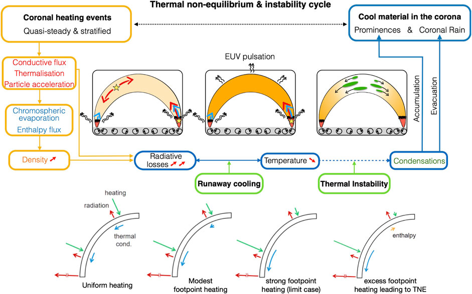
FIGURE 1. TNE-TI cycle. Top: A sketch showing the main physical processes that participate in the thermal non-equilibrium (TNE) and thermal instability (TI) cycle. Orange and blue boxes denote the heating and cooling phases, respectively. The 3 inset images with loops denote 3 instances through the cycle, ordered according to the TNE-TI sequence: heating events (yellow stars) occur either high up or lower down in the atmosphere. Thermal conduction (red arrows) distributes the heating. Chromospheric evaporation occurs (blue arrows), leading to dense loops (particularly in the case of footpoint heating). The loops get dense (second loop image) and emit strongly. Radiative cooling (wiggly black arrows) dominates over heating, leading to successive peaks of emission in gradually cooler EUV passbands (an EUV pulsation is observed in this stage). Under the right conditions (cf. §2.1.1) this process leads to runaway cooling. TI sets in, producing condensations (third loop image) that either accumulate in the corona to form prominences or fall as coronal rain. The loop evacuates and the cycle restarts. Adapted from Figure 3 of Antolin (2020). Bottom: Sketch explaining the main physical processes at play when achieving thermal stability in a loop (half a loop is shown here, for simplicity), and the onset of TNE for the case of strongly stratified heating. Adapted from Figures 1, 3 of Klimchuk and Luna (2019) (© AAS. Reproduced with permission).

The heating is generally considered stratified when most of the heating is concentrated at the feet of a magnetically-closed structure, up to 20% of its height. Klimchuk and Luna (2019) have shown that this stratification is a necessary condition in order to trigger TNE, but not a sufficient one as it was shown by various numerical experiments. Klimchuk and Luna (2019) derived two formulae quantifying the necessary conditions for TNE to occur. The heating must be small at the loop apex compared to the heating in the transition region:

$\frac{Q_{\mathit{min}}}{Q_{\lambda }}<{\left(1+\frac{c_1}{{\mathrm{\Gamma }}_{\lambda }}\right)}^{-1},(1)$

where

${\mathrm{\Gamma }}_{\lambda }\equiv \frac{A_{\lambda }}{A_{tr}},(2)$

and

$c_1\equiv \frac{R_{tr}}{R_c}(3)$

Q_min and Q_λ are, respectively, the volumetric heating rates at the loop apex and at one heating scale length above the transition region, λ corresponds to one heating scale length along the coronal loop (from the top of the transition region), A_λ and A_tr are the cross-sectional areas averaged along the first heating scale length and transition region sections, respectively, R_tr and R_c are the radiative losses per unit area, integrated along the coronal and transition region sections, respectively.

The second formula derived by Klimchuk and Luna (2019) states that the asymmetries in the loop should not be too great for TNE to occur:

$\left(\frac{Q_s}{Q_w}\right){\left(\frac{{\lambda }_s}{{\lambda }_w}\right)}^2\left(\frac{{\mathrm{\Gamma }}_s}{{\mathrm{\Gamma }}_w}\right)\left(\frac{{\mathrm{\Gamma }}_w+2}{{\mathrm{\Gamma }}_s+2}\right)<{\left[1-4.3\times 10^2\frac{A}{A_w}(1-\delta )\frac{L}{{\lambda }_s}\right]}^{-7/2}(4)$

where

$\delta =\left(1+\frac{c_1}{{\mathrm{\Gamma }}_s}\frac{Q_{\mathit{min}}}{Q_s}\right)(5)$

L is the coronal loop half-length, the indexes S and W correspond to the strongly heated footpoint and weakly heated footpoint, respectively. A and A_w are the cross-sectional areas at, respectively, the location of minimum heating and one heating scale length above the transition region on the weakly heated side. The area ratio is typically between 1 and 2.2.

The parameter space for heating and geometrical properties for coronal loops is extensive. One-dimensional hydrodynamical simulations have been the preferred numerical description to explore this parameter space due to field-aligned dominated dynamics but also due to computational limitations (see Reale, 2014, for a review on loop modeling). These are rather simple models but they allow to explore extensively the global features of TNE. In the solar corona the magnetic Reynolds number is very high, which means that the plasma is confined in magnetic structures, closed-field lines in the case of coronal loops. In the β ≪ 1 conditions of the solar corona, the magnetic field serves as a guide for the plasma that is considered to be a compressible fluid. The equations for the conservation of mass, momentum and energy are solved numerically. The thermal conduction, radiative losses and heating, the latter in the form of ad hoc functions describing the volumetric heating rate along the loop, are taken into account in order to study the plasma response. However, even in 1D, all the possible parameters cannot be explored simultaneously, and important nonlinear effects may be missed. Also, this 1D approximation cannot explore the reasons for the observed cross-field structuring of the coronal plasma. The main parameters usually considered are stated below.

The Loop Length

Intuitively, longer loops will lead to TNE cycles with longer periods as the volume of the flux to fill from the chromospheric reservoir at the footpoints increases, and radiative cooling timescales are longer due to the lower densities on average. This is clearly shown in e.g., Froment et al. (2018). Starting form the classical RTV scalling laws (Rosner et al., 1978), it was also shown analytically by Auchère et al. (2014) that the characteristic evolution time of loops should be correlated with their length, regardless of TNE occurrence.

The Loop and Heating Geometry

Müller et al. (2003, 2004) were the first to explore the influence of the heating scale height, that we will note here λ, or “damping length” in their papers, on the thermal evolution of a coronal loop. They showed that for the same loop length L, different λ would lead to TNE with different periods and maximum temperatures and densities, including no TNE at all. Before that, Karpen et al. (2001) showed that only large enough structures would lead to prominences for the similar reason that the λ/L should not be too great to foster TNE. The typical parametrization used for describing the loop volumetric heating follows that introduced by Serio et al. (1981): H = H_base  exp(−s/λ), with H_base the volumetric heating at the footpoint of the loops and s the curvilinear abscissa along the loop (see Mikić et al., 2013; Froment et al., 2018; Johnston et al., 2019; Pelouze et al., 2022, for more details).

In numerical simulations exploring condensations phenomena, the loop geometry has for a long time chosen to be exclusively semi-circular (e.g., She et al., 1986). On top of that, the heating geometry, represented by the heating scale height in each loop leg, was symmetric (e.g., Müller et al., 2003; Klimchuk et al., 2010). Even the loop cross-section was chosen to be constant, even though the expected expansion of the magnetic field with height has important consequences in terms of enthalpy and thermal conduction. This was based on the observed moderate to no expansion of coronal loops in EUV (Klimchuk, 2000; Watko and Klimchuk, 2000). Recent studies at high resolution in the EUV further support the circularity of the loop cross-section and the lack of expansion (Klimchuk and DeForest, 2020). Numerical studies have suggested that this may be an apparent effect caused by a combination of temperature, density, cross-section area variation and instrumental factors (e.g., Peter and Bingert, 2012; Malanushenko and Schrijver, 2013).

Mikić et al. (2013) were the first to explore different geometries of loops and heating, especially different degrees of asymmetry. They investigate different configurations that deviate from a semi-circular loop, exploring constant and non-constant loop cross-sections, symmetric and asymmetric heating profiles with different heating strengths. They showed that the previous oversimplifications in loop simulations, namely not taking into account the full range of loop geometrical properties, can lead to unrealistic loop observables (see Klimchuk et al., 2010; Lionello et al., 2013, for more details and Section 3.3). The inclusion of an expanding area cross-section with height greatly increases the thermal conduction flux into the transition region, thereby increasing the radiative losses there and leading to greater chromospheric evaporation and thus greater coronal density. The onset of TNE is therefore more easily achieved for loops expanding with height. Exploring loop and heating geometrical parameters, Mikić et al. (2013) actually showed that asymmetries lead to persistent siphon flows that can provide an important source of energy (in the form of an enthalpy flux) to the cooling coronal plasma, as well as severely reducing the time it stays in the coronal region. Such asymmetries can therefore play a central role in TNE onset, strongly vary the TNE cycle properties, as well as the cooling rate and morphology of the condensations. Through this process, it was observed that the catastrophic cooling of condensations down to chromospheric temperatures could therefore be aborted, leading to “incomplete” condensations for which the temperatures remain at transition region temperatures. For these cases, the apex temperature of the loop was found to cool down to 1 MK only, with a density of at most 5 × 10⁹ cm⁻³.

In Froment et al. (2018), these results were revisited following the discovery of long-period intensity pulsations (section 2.2.1). Using realistic loop geometries from photospheric magnetic field extrapolations (different L, asymmetries and loop expansion), the authors explored the heating parameter space by varying λ, and the volumetric heating rate at the foopoints and at the apex. They found that in principle any loop geometry could lead to TNE but only under very specific geometrical heating conditions varying from a loop to another. The need of a specific match between the loop geometry and the heating geometry in order to produce TNE reveals that for a particular loop geometry, the domain where TNE is possible is rather limited in the heating parameter space as it can be seen on the left of Figure 2. On the right panel of Figure 2, we show two simulations that are extracted from Froment et al. (2018) parameter space exploration. Both simulations use the same heating parameters with a symmetric heating function, but a different loop geometry. While the simulation with Loop A (semicircular loop) produces TNE with coronal rain-like signatures, the simulation with Loop B (asymmetric loop) shows no TNE signatures. This need of a specific match between the loop geometry and the heating geometry is relaxed when the heating strength increases, as we will see below and on Figure 2 as the TNE domain increases for each loop geometry when the heating rate increases.

FIGURE 2

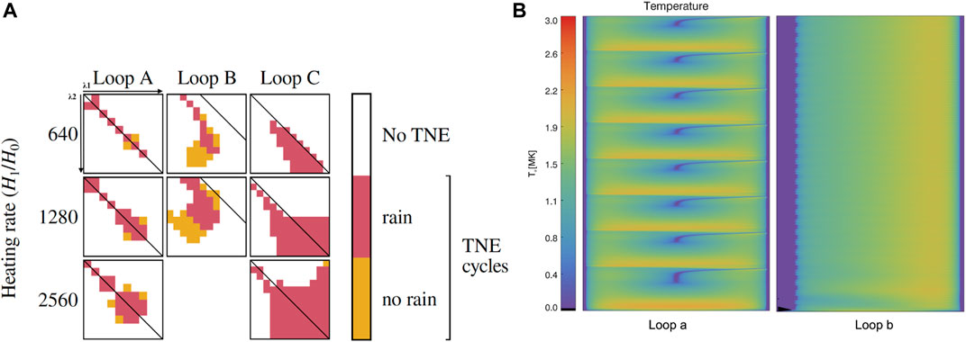
FIGURE 2. Left: (A) This figure is adapted from Figure 7 of Pelouze et al. (2022). It shows the parameter space explored in the simulations of Froment et al. (2018). Three loops geometry were considered for an extensive heating rate and scale height scan using 1D hydrodynamic simulations. Each big square represents a set of simulations, the heating scale heights for each loop leg is varying on the x-axis (λ₂) and y-axis (λ₁) and from the top-left to the bottom-right. These variations are ranging from 2% to 18% of the three loop lengths. Each small square corresponds to one simulation. The diagonal line shows the cases where λ₁ = λ₂, i.e. symmetric heating cases. Loop A was a semicircular loop with L = 367 Mm, while Loop B and Loop C were geometries coming from magnetic field extrapolations. Loop B is strongly asymmetric with L = 367 Mm and Loop C moderately asymmetric with L = 137 Mm. Here the heating rate H₁/H₀ corresponds to H_base/H_background. (B) Figure adapted from the results of Froment et al. (2018), both simulations have λ₁ = λ₂ = 29.4 Mm, L = 367 Mm, H₁ = 6.4 × 10^–5 W m⁻³, on the left with geometry of Loop A, on the right that of Loop B. The same color scale is used for the temperature. The x and y-axis represent, respectively, the position along the loop length and 3 days of loop evolution.

Pelouze et al. (2022) show that the asymmetric loops are less likely to produce complete condensations. Indeed, it was found that more stringent conditions on the heating geometry are needed for this purpose when geometrical asymmetries are considered. This can be understood from the fact that stronger geometrical asymmetries more readily lead to siphon flows. This condition was quantified through analytical formulae (Klimchuk and Luna, 2019). The authors found that “as a rough rule of thumb,” asymmetries between the two values of the heating parameter λ for a loop should be less than a factor of 3 in order to produce TNE cycles (see Eqs 1, 4).

The Strength of the Volumetric Heating at the Footpoint

In the parametrization of the volumetric heating, the parameter H_base has also a significant influence on the generation of TNE cycles and their properties. It was shown by Froment et al. (2018) that the TNE cycles are more common when H_base increases and that these cycles tend to produce more complete condensations rather than incomplete condensations. This is expected since the average coronal density increases with footpoint heating due to stronger chromospheric evaporation (see section 3.1). This increase of coronal density then shortens the radiative cooling timescale and increases the growth of thermal modes leading to complete condensations.

Klimchuk and Luna (2019) draw a similar conclusion analytically. The ratio of the apex to footpoint volumetric heating rate should be less than 0.1 in order to get TNE. The heating at the apex is usually parametrized by a constant: H = H_background + H_base  exp(−g(s)/λ). Here g(s) = max{s − Δ, 0}, with Δ the thickness of the chromosphere (see Mikić et al., 2013; Froment et al., 2017). With such an additional term H_background + H_base becomes the new volumetric heating in the chromosphere and H_background the value to which H tends to at the apex (only if $\lambda \ll \frac{L}{2}-\mathrm{\Delta }$).

The So-Called Background Heating Term: Volumetric Heating at the Loop Apex

This background heating term is almost always considered in 1D hydrodynamical simulations, mostly to achieve hydrostatic equilibrium prior to the start of an experiment. Its value is generally small compared to H_base and thus was rarely considered to play an important role. However, Johnston et al. (2019) showed that this parameter has in reality a great influence on the onset and characteristics of the TNE cycles, in support of Klimchuk and Luna (2019). This is clearly shown in Figure 3, where the TNE period is seen to vary greatly when the background heating is varied in the range of 10^–5 − 10^–4 J m⁻³ s⁻¹, and when it is larger than $\approx 10^{-4}$J m^{−3 s−1} TNE is entirely suppressed. This is of particular importance for 3D MHD simulations, where large diffusion coefficients are usually used in favour of numerical stability and computational efficiency. Such large diffusivity can act as a background heating term, even though it is artificial and therefore non-physical.

FIGURE 3

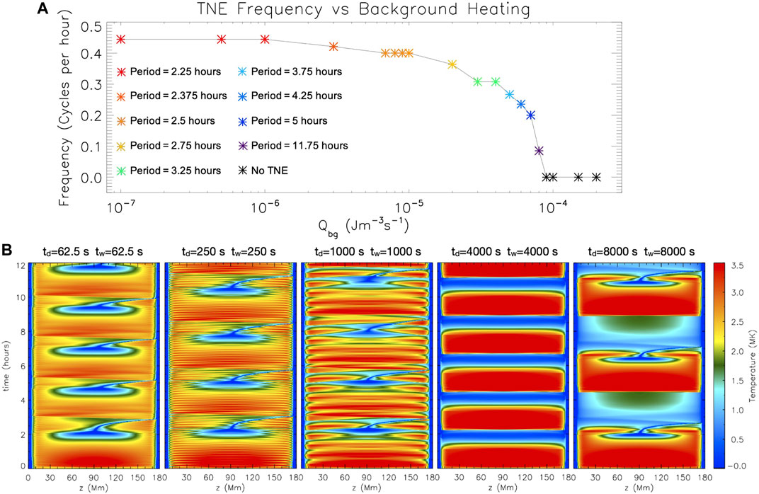
FIGURE 3. (A) Frequency of the TNE cycle for one-dimensional simulations of a 180 Mm long loop with footpoint heating (located at a height of 12.5 Mm) for which the heating events last a time of t_d = 125 s and with a waiting time of t_w = 125 s between events but with a varying value of the background heating term (constant along the loop). (B) 5-layer panel: time-distance diagrams of the temperature variation along the loop for one-dimensional simulations of the same loop but with varying values of t_d and t_w. For further details please see Johnston et al. (2019) (adapted from Figures 6, 10 of that paper, reproduced with permission © ESO).

The Heating Timescale

In TNE simulations, the volumetric heating rate is generally constant for the full duration of the simulation. It is important to note that the quasi-steadiness of the heating is a crucial criterion in order to maintain TNE cycles as it was pointed out by Peter et al. (2012). Without a sufficiently high frequency heating there seems to be not enough density supply to maintain the production of condensations. The effect of periodic or randomly occurring heating events on TNE cycles has been explored to some extent (see e.g., Mendoza-Briceño et al., 2002, 2005; Antolin et al., 2008; Susino et al., 2010). Johnston et al. (2019) show that TNE is produced when the time between each heating event t_w is lower than the radiative cooling time of the loop. When these timescales are on the same order, condensations may still occur if the heating is sufficiently strong. However, the observed periodicity in the cycles is then governed by the heating timescale, meaning that TNE stops occurring. This sets in evidence the fact that condensations such as prominences or coronal rain can occur without TNE whenever the heating varies significantly enough to impose its own timescales.

As seen above, TNE crucially depends on the coronal density, and factors such as the heating scale length or background heating naturally have a great impact on the density. On the computational side, a major parameter that also affects coronal density is spatial resolution, as demonstrated by Bradshaw and Cargill (2013). Indeed, coarse spatial resolution affects the amount of energy that is radiated away in the transition region, leading to lower levels of chromospheric evaporation and therefore lower coronal density. Johnston et al. (2019) show that in order to properly capture the radiative losses in the transition region and the resulting enthalpy flux into the corona through the process of chromospheric evaporation a spatial resolution of at least 2 km should be achieved in the transition region. This is of course prohibitive for 3D numerical simulations with uniform grids and challenging even for codes with adaptive grids. Fortunately, numerical methods now exist that circumvent this process by either artificially broadening the transition region (Mikić et al., 2013) or by adapting a jump condition that properly captures the radiation in the unresolved transition region (Johnston et al., 2017; Johnston and Bradshaw, 2019; Johnston et al., 2021; Zhou et al., 2021), leading to correct results even with coarse resolution.

We focused here on 1D studies that are very useful to comprehend the influence of the different geometrical and heating parameters. However, we note that 3D MHD simulations of TNE have been performed (Mok et al., 2016). In these simulations the heating was based on the turbulent Alfvén wave dissipation theory (Rappazzo et al., 2008), with the volumetric heating rate depending on the loop’s length, the magnetic field strength and the plasma density. Such simulations are important for proper comparison with observations since 3D aspects (such as line-of-sight superimposition) are taken into account in the forward modelling. However, these simulations are similar to most of the 1D studies mentioned above in the sense that the magnetic field structure is kept fixed during the simulation. Moschou et al. (2015), Xia et al. (2017) have successfully simulated in 3D MHD a (fixed) loop arcade undergoing 1 cycle of TNE, together with catastrophic cooling and the accompanying coronal rain. More recently, Li et al. (2022) in 2.5D MHD at sufficiently high resolution have managed to produce several TNE cycles with accompanying coronal rain in a fixed loop arcade. However, it remains a challenge for future studies to self-consistently include the magnetic field evolution in multi-dimensional simulations that are long enough to include several EUV pulsations (see Section 2.2.3 and Section 4.1). 

2.1.2 Local Scales: Thermal Instability

The formation of cool material in hot environments has long been associated with thermal instability (TI). This has been the case primarily in the study of the interstellar, intracluster and circumgalactic media, where cool structures down to a few K such as molecular clouds or galactic loops are observed to form in 10⁷–10⁸ K environments (e.g., Zanstra, 1955; Fukui et al., 2006). These environments are usually assumed to be in hydrostatic and thermal balance because of their long lifetimes and validity of the virial theorem. In this context, analytical work (Field, 1965; Parker, 1953; Claes and Keppens, 2019) and simulations (Koyama and Inutsuka, 2000; Cox, 2005) have shown that the MHD thermal mode can become unstable and give rise to the formation of very cool and dense condensations (see Figure 4), with a filamentary morphology due to the presence of magnetic fields introducing anisotropic thermal conduction (Sharma et al., 2010). The detailed conditions under which this happens vary depending on the environment.

FIGURE 4

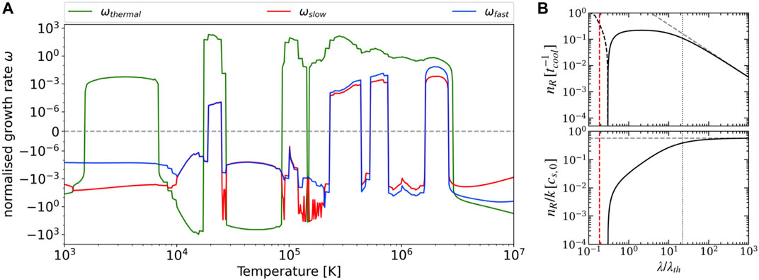
FIGURE 4. (A) Growth rate (imaginary component of frequency) of the solutions of the dispersion relation for an infinite, homogeneous magnetised plasma in equilibrium for an angle of 45° between the wave vector and magnetic field, including optically thin radiative losses, parallel and perpendicular thermal conduction (and neglecting the effects of gravity and resistivity) as a function of temperature. The equilibrium values are a density ρ = 9.64 × 10^–14 g cm⁻³, a magnetic field strength of B = 10 G and a length scale of L = 10⁸ cm. Green, red and blue curves denote the thermal, slow and fast mode growth rates, respectively. This plot is adapted from Figure 1 in Claes and Keppens. (2019) (reproduced with permission © ESO) but modified by N. Claes to include the more modern cooling curve by Schure et al. (2009), extended to low temperatures using Dalgarno and McCray (1972) (see also Claes and Keppens, 2021, for more details). (B) Growth rate of the entropy mode n_R (top) and n_R/k (cf. Eq. 6) as a function of perturbation wavelength λ = 2π/k. The dashed portion of n_R denotes negative values corresponding to stabilisation due to thermal conduction (the Field’s length is shown in red). The grey dashed line denotes the asymptotic growth of the entropy mode when k → 0 (cf. Eq. 12). The dotted vertical lines denotes λ_c ≈ 22.3λ_th (from Figure 1 in Waters and Proga, 2019, © AAS. Reproduced with permission).

For instance, under the assumption of radiative cooling compensated locally by a heating function with only parallel thermal conductivity included, the localised catastrophic cooling produced by thermal instability can be investigated in the linear regime of the process through the following dispersion relation, which governs the entropy (or thermal) mode and two acoustic modes. Following (Waters and Proga, 2019), we have:

$n{\left(\frac{n}{k}\right)}^2+\frac{N_p}{t_{\text{cool}}}{\left(\frac{n}{k}\right)}^2+n{c}_{s,0}^2+\frac{N_p}{\gamma t_{\text{cool}}}{c}_{s,0}^2=0,(6)$

where we assume perturbations of the form   exp(nt + ik ⋅x), with n = n_R + in_I and k = 2π/λ the wavenumber of the perturbation, $t_{\text{cool}}=\mathcal{E}/\mathrm{\Lambda }$ is the timescale for the gas to lose its thermal energy $\mathcal{E}=c_{V}T$, $c_{s,0}=\sqrt{\gamma k_{B}T/\bar{m}}$ is the background sound speed ($\bar{m}$ the mean particle mass) evaluated in the equilibrium state, and N_p and N_f are dimensionless quantities defined as:

$\begin{array}{ccc}\hfill N_{\rho }& \equiv \hfill & \frac{T_0}{{\mathrm{\Lambda }}_0}{\left(\frac{\partial \mathcal{L}}{\partial T}\right)}_{\rho }+{\left(\frac{{\lambda }_F}{\lambda }\right)}^2,\hfill \end{array}(7)$

$\begin{array}{ccc}\hfill N_p& \equiv \hfill & \frac{T_0^2}{{\mathrm{\Lambda }}_0}{\left(\frac{\partial (\mathcal{L}/T_0)}{\partial T}\right)}_p+{\left(\frac{{\lambda }_F}{\lambda }\right)}^2.\hfill \end{array}(8)$

The subscript ρ, p denote the thermodynamic variable that is held fix when measuring the net cooling change $\mathcal{L}=\mathrm{\Lambda }-\mathrm{\Gamma }$, where Λ denotes the radiative cooling function and Γ denotes the heating function. The Field’s length λ_F is defined as (Begelman and McKee, 1990):

${\lambda }_F={\left.2\pi \sqrt{\frac{\kappa T}{\rho \mathrm{\Lambda }}}\right|}_0,(9)$

where κ is the thermal conduction coefficient and the thermodynamic variables ρ, T are evaluated in the equilibrium state. Field (1965) showed that perturbations with wavelengths shorter than λ_F are suppressed due to thermal conduction (see right panels in Figure 4).

The unstable entropy modes require the growth rate n_R > 0 with n_I = 0, and Eq. 6 reduces to:

$n_R=-\frac{N_{\rho }}{t_{\text{cool}}}\frac{u^2+R{c}_{s,0}^2}{u^2+c_{s,0}^2},(10)$

where u ≡ n_R/k describes the speed of inflow gas feeding the condensation, and R ≡ N_p/N_ρ denotes the ratio of the cooling rate derivatives. Critical values of R distinguish the various regimes of TI. The isochoric regime can be obtained by setting k → 0 and u → ∞. In this case, λ_F/λ goes to 0, leading to n_R → constant and to N_ρ < 0, that is, from Eq. 7:

${\left(\frac{\partial \mathcal{L}}{\partial T}\right)}_{\rho }<0.(11)$

If, instead, u → constant as k → 0 and n_R → 0 (the long wavelength perturbation regime), we obtain the asymptotic growth of the entropy mode in the isochoric regime:

$n_R=k{c}_{s,0}\sqrt{-R},\text{with}u=\pm c_{s,0}\sqrt{-R}.(12)$

In the isobaric regime, the condensations are characterised by very low inflow speeds u < < c_s,0. Eq. 10 then reduces to N_p > 0 (requiring n_R > 0), that is:

$\frac{T_0^2}{{\mathrm{\Lambda }}_0}{\left(\frac{\partial (\mathcal{L}/T_0)}{\partial T}\right)}_p<{\left(\frac{{\lambda }_F}{\lambda }\right)}^2,(13)$

which is known as Balbus criterion for TI (Balbus, 1986) (or the generalised isobaric criterion). The isobaric TI applies to perturbations with wavelengths on the order of the thermal length λ_th:

${\lambda }_{\text{th}}\equiv (c_s{t}_{\text{cool}}){|}_0,(14)$

which corresponds to the distance sound waves propagate in a cooling time (Inoue and Omukai, 2015). More precisely, Waters and Proga (2019) have shown that acoustic modes become unstable for λ > λ_c ≈ 22.3λ_th. The critical wavelength λ_c that characterises this transition is approximated by:

${\lambda }_c\approx \frac{2\pi }{|N_{\rho }|}{\lambda }_{th}\sqrt{-B/R},(15)$

where B = (27/4) (R − 1/3)²–1. This critical wavelength may be thought as a more general expression for the “acoustic Field’s length” described in Kolotkov et al. (2021). In other words, the isobaric instability criterion always applies to the entropy mode and to acoustic modes for λ > λ_c.

As shown by Waters and Proga (2019), Claes and Keppens (2019), acoustic waves are found to be efficient triggers of (or become themselves) condensation modes. Similar results have been obtained by Zavershinskii et al. (2021), which show that the properties of acoustic and thermal modes become mixed when a feedback is allowed from unbalanced heating and cooling processes (a regime known as thermal misbalance). The evolution of the condensations depends on one hand on the thermal instability regime, and in particular on the inflow velocity u = n_R/k, which can lead to fragmentation effects due to strong oscillations in size, temperature and density. On the other hand, Hermans and Keppens (2021) have shown that the cooling curve chosen for the treatment of the radiative losses, and in particular the treatment at low temperatures (<20 000 K), greatly varies the growth rate of the instability and the morphology of the condensations. This theory has been applied to the formation of coronal rain and prominences in the solar context. Numerical simulations have shown that the formation of condensations in the solar context seems to agree well with the isochoric thermal instability (Xia et al., 2011; Moschou et al., 2015).

However, an important difference between a hot environment such as the ISM or ICM and the solar corona is the initial assumption of hydrostatic and thermal equilibrium for the study of thermal instability. Indeed, the solar corona, and in particular the active regions where coronal rain is usually found, are far from hydrostatic equilibrium (Aschwanden et al., 2001). As discussed in the previous section, footpoint heating usually found in these regions (cf. section 3.2) set coronal loops in a state of TNE, which involves strong flows due to the cyclic heating and cooling. In this scenario, it has been argued that TNE alone can explain the formation of condensations (Antiochos et al., 1999), and that the usual stability analysis approach for assessing the existence of condensation modes is invalid since the initial condition of thermal equilibrium is never achieved (Klimchuk, 2019). On the other hand, it has been debated that while globally coronal loops may not be in equilibrium but in a TNE state, locally thermal instability takes place in an approximate state of equilibrium (Antolin, 2020). The argument is based on the fact that during the cooling stage of the TNE cycle and prior to the catastrophic cooling stage, all flows are subsonic and the loop’s evolution is slow enough to be in approximate thermal balance. Formally, this can be analysed in terms of thermal misbalance (due to heating-cooling misbalance) under specific timescales, and the occurrence of thermal instability under thermal misbalance (and its back-reaction on the wave modes) is an active new branch of research with very interesting seismological applications (Kolotkov et al., 2020; Duckenfield et al., 2021; Kolotkov et al., 2021; Zavershinskii et al., 2021). Non-adiabatic MHD spectroscopy codes are now available, such as “Legolas” (Claes et al., 2020), that take into account thermal misbalance and allow to quantify the stability of the wave modes in one-dimensional setups. Using this tool, Claes and Keppens (2021) show that thermal instabilities are unavoidable in the solar atmosphere, and that all modes (thermal, slow and fast) may exhibit unstable behaviour.

2.2 Observational Properties

2.2.1 Multi-Scale EUV Cooling Observations and Relationship With Thermal Non-Equilibrium-Thermal Instability

2.2.1.1 The Widespread Coronal Cooling

EUV cooling is a well-known feature of the corona. As reported by many observational studies and understood through numerical simulations (e.g., Warren et al., 2002; Winebarger et al., 2003; Winebarger and Warren, 2005; Ugarte-Urra et al., 2006; Mulu-Moore et al., 2011; Warren et al., 2011; Viall and Klimchuk, 2011, 2012, 2017), the corona is observed to be in a constant and widespread state of cooling. Indeed, although heating events have to happen in order to sustain the corona at its characteristic high temperatures, only the cooling events are usually observable (at least with the current instrumental capabilities). Different types of loop models (TNE, nanoflare storms, etc) all show that the heating phases occur at a low plasma density, which means at low emission measure, making its detectability in the EUV challenging. However, during the cooling phases the density is high and the radiative cooling times are longer, making it possible to observe the temperature variations. These are observed gradually in different EUV lines and/or passbands, according to the peak temperature response of these lines/passbands. This state of cooling is thus there, regardless of the heating mechanism and its properties.

2.2.1.2 The Deconstructed Puzzle of EUV Manifestations of TNE

As it will be detailed in Section 2.2.3 the first and most well-known manifestations of TNE and/or TI in the solar atmosphere are prominences and coronal rain, that were discovered in chromospheric lines such as Hα. Coronal counterparts of TNE-TI cycles, in EUV lines, have been more discrete and not straightforward to reveal. However sparse, EUV manifestations of TNE were observed quite early following the discoveries of their cool cousins, even though they were not directly reported as such. Foukal (1978) reported dark absorption features in the EUV passbands that were related to coronal rain events. With the Coronal Diagnostic Spectrometer (CDS, Harrison et al., 1995) onboard the Solar and Heliospheric Observatory (SoHO, Domingo et al., 1995), Kjeldseth-Moe and Brekke (1998) observed an important variability, stronger at lower transition region temperatures, in a few loops where they also found downflows in the O V lines that reveal material at chromospheric temperatures. EUV variability characteristic of cooling, in relation with coronal rain, was also found in the Transition Region and Coronal Explorer (TRACE, Handy et al., 1999) observations by Schrijver (2001). In this study, time delays were reported between the light curves of coronal channels and transition region/chromospheric channels. This observation thus provided evidence of cooling from coronal to chromospheric temperatures. Cool material was reported falling toward loop footpoints by De Groof et al. (2004) in the 304 Å   channel of the Extreme Ultraviolet Imaging Telescope (EIT, Delaboudinière et al., 1995) and was later associated to coronal rain in De Groof et al. (2005). However no imprint at higher temperatures were reported. O’Shea et al. (2007) with SoHO/CDS reported a decrease in the intensities of the coronal lines simultaneous with the appearance of plasma condensations.

The rapid cooling trend and increase in variability across transition region lines was further elucidated with Hinode/EIS observations in the Mg VI 269 Å  (0.4 MK) and Si VII 275 Å  (0.63 MK) lines by Ugarte-Urra et al. (2009), seen in Figure 5. An increase in strand-like structure (and respective decrease in diffuse, more extended EUV emission) is clear, associated with the fan-like peripheral cool loops. Similar reports have been made with Hinode/EIS and SDO/AIA, sometimes accompanied by dark or bright downflowing features interpreted as coronal rain (Tripathi et al., 2009; Kamio et al., 2011; Orange et al., 2013).

FIGURE 5

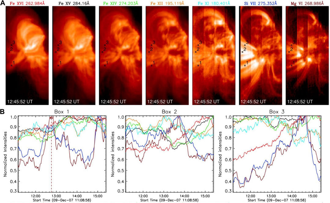
FIGURE 5. (A) An active region observed with Hinode/EIS in multiple spectral lines, reported by Ugarte-Urra et al. (2009), ordered from left to right in decreasing order of temperature formation (starting at 2.62 MK with Fe XVI 262.98 Å  and ending at 0.4 MK with Mg VI 269 Å). (B) Light curves in the various spectral lines integrated over Boxes 1, 2 and 3, shown in the top panels, located on peripheral cool loops. See Ugarte-Urra et al. (2009) for more details (adapted from Figure 5 in that paper, © AAS. Reproduced with permission).

2.2.1.3 Long-Period Intensity Pulsations as a Coronal Manifestation of Thermal Non-Equilibrium

Major steps, both observational and theoretical, toward bringing together the pieces of the multi-scale observations of TNE-TI puzzle happened in the past few years. Using more than a solar cycle of observations with SoHO/EIT, Auchère et al. (2014) reported the widespread occurrence of long-period intensity pulsations in the corona using the 195 Å passband that had both a sufficient cadence of 12 min and an almost continuous coverage of the full disk corona from January 1997 to July 2010. These quasi-periodic EUV variations have periods ranging from 2 to 16 h (same as the range explored by the authors) and are most remarkably very common in coronal loops (about 25% of the events). They can be observed continuously in the same area for up to 6.5 days, a duration only limited by observational constraints. Using the Atmospheric Imaging Assembly (AIA, Lemen et al., 2012) on board the Solar Dynamics Observatory (SDO, Pesnell et al., 2012), Froment et al. (2015) confirmed the existence of such widespread pulsations, and through thermal analyses connected them to evaporation and condensation cycles in coronal loops. The discovery of long-period EUV pulsations was critically assessed in Auchère et al. (2016a) with Fourier and wavelets analysis. The high confidence in these detections was demonstrated using a proper noise model, global confidence levels and evidencing no source of artefacts such as pre-filtering of the data.

These studies brought evidence, for the first time, of what has been predicted by TNE simulations for decades: TNE cycles are periodic and they have a strong manifestation in the coronal EUV observations through the observation of pulsations. In parallel, using the wide temperature range observation capabilities brought by coordinated Hinode (Kosugi et al., 2007), SDO and the newly Interface Region Imaging Spectrograph (IRIS, De Pontieu et al., 2014) observations at the time, Antolin et al. (2015) uncovered the multi-thermal aspects of coronal rain, spanning chromospheric, transition region and coronal temperatures with a progressive cooling through them (see section 2.2.3). On the modelling side, a series of papers (Lionello et al., 2013; Mikić et al., 2013; Winebarger et al., 2014) demonstrated that TNE, that was previously considered to be a sporadic phenomenon, mostly linked to prominences and coronal rain, could occur in coronal loops with standard properties and explain several observational constraints (see Klimchuk et al., 2010; Lionello et al., 2013, for the key loop observables).

While the widespread occurrence of long-period intensity pulsations was confirmed in Froment (2016), its relationship with TNE was confirmed by Froment et al. (2017) confronting the SDO/AIA observations to 1D hydrodynamic TNE simulations. A comparison of the synthetic intensities derived from such simulations and the observed intensities is presented in Figure 6. To the best of our current knowledge, no other model besides TNE is able to reproduce the key properties of the observed long-period intensity pulsations. The X-ray emission in the model of Imada and Zweibel (2012) shows pulsations whose periods are compatible with those observed by Auchère et al. (2014) and Froment (2016), given the length of the loops studied. However, in these simulations the temperature and the density show a different correlation than that produced from the usual TNE, allowing a differentiation based on observations. Auchère et al. (2016b) demonstrated that properties of the EUV signal itself is consistent with TNE. Indeed the imprint of the long-period intensity pulsations on the Fourier spectra are consistent with a succession of periodic pulses of random amplitudes (rather than oscillations linked to vibration modes). As we have seen in Section 2.1.1, the variation of loop and heating geometries and heating magnitudes will impact the average temperature and density reached in the TNE cycles and thus ultimately the EUV intensity. This means that even without considering the very important line-of-sight effects, TNE cycles will likely not repeat themselves identically and we should thus expect varying amplitudes and possibly periods (see Section 4.1).

FIGURE 6

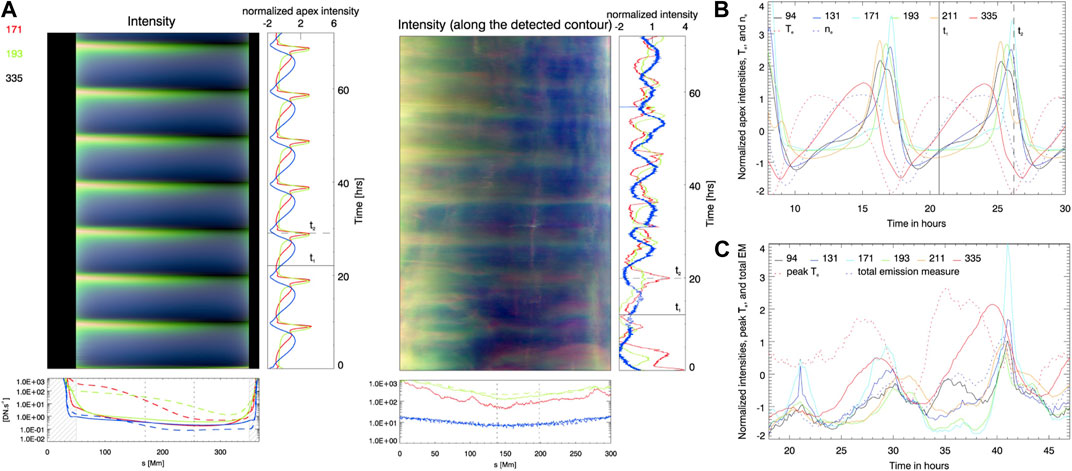
FIGURE 6. Long period-intensity pulsations in the SDO/AIA coronal channels and comparison with simulations. (A) Simulation of EUV intensities from a 1D hydrodynamical simulation of TNE. Middle: EUV intensities for the main loop bundle studied in Froment et al. (2015). See Froment et al. (2018) for more details. Both panels are adapted from Figure 17 of that paper. (B) Synthetic intensities from a 1D hydrodynamic simulation. The dotted lines represent the temperature and the density, respectively. (C) Intensities from the observations. The dotted lines represent the peak temperature of the DEM and the total emission measure, respectively. Both panels are adapted from Froment et al. (2017) (Figures 9, 12, © AAS. Reproduced with permission). See the original papers for more details.

2.2.1.4 Thermal Properties

The thermal structure of loops exhibiting long-period intensity pulsations was investigated combining Differential Emission Measure (DEM) analysis with time lag analysis. The DEM represents the amount of emitting plasma along the line-of-sight as a function of the temperature. In active regions, the DEM generally follows a power law in the low temperature range (below the DEM peak, e.g. Warren et al., 2011). Using the DEM inversion method of Guennou et al. (2012, 2013), Cheung et al. (2015), Froment et al. (2015), and Froment et al. (2020) showed that long-period intensity pulsations events can show a periodic variation of the DEM slope (i.e., the power law index). Even though this parameter is usually poorly constrained in the DEM inversion process, this behaviour is consistent with synthetic DEMs produced with numerical simulations of loops in TNE (private communication, Cooper Downs). DEM analysis also revealed a time delay between the temperature (via the peak temperature of the DEM) and density (via the total emission measure, proportional to the density squared). This time delay combined with the periodicity of their evolution strongly matches the TNE predictions, and thus constitute strong evidence of TNE.

Using the time-lag method developed and popularized by Viall and Klimchuk (2012), both observational and modelling studies (Froment et al., 2015; Winebarger et al., 2016; Auchère et al., 2018; Froment et al., 2020) showed that long-period intensity pulsations and TNE are consistent with the widespread EUV cooling patterns observed in the solar corona.

2.2.1.5 The Occurrence of Long-Period Intensity Pulsations

The discovery of widespread long-period intensity pulsations in the corona as a manifestation of TNE led to two major puzzles: How these cycles, linked to a particular heating distribution in space and time, can be maintained for several days given the stochasticity of the physical conditions on the Sun? Auchère et al. (2014) estimated that about 50% of the active regions of solar cycle 23 underwent long-period intensity pulsations. Why are some loops entering this particular thermodynamic regime while others do not?

While the first question remains open (see Section 4.1), the second one was tackled by Froment et al. (2018) by exploring the heating parameter space for several loops geometries with 1D hydrodynamical simulations (see Section 2.1.1). The authors found that for each geometry the domain where TNE is found in the heating parameter space is limited and that these geometrical heating conditions are case dependent. This explains why every loop bundle does not show quasi-periodic intensity pulsations. Within the same active region for example, the heating conditions imposed at low altitude in the chromosphere may be similar from a loop bundle to a neighboring one. However, only the loop bundle that has a loop geometry compatible with the heating conditions will undergo TNE. It is also very likely that the line-of-sight integration may in some cases prevent clear detections. As shown in Section 4.1, the current method used to detect these pulsations is very likely leading to non-exhaustive statistics, and more like a tip-of-the-iceberg scenario.

It is important to note that the loops showing long-period intensity pulsations evolve on average in phase across the same bundle (Froment et al., 2015). While these loops may have similar geometries and heating conditions at their footpoints, their lengths are expected to be different (shorter in the inner part of the bundle), and thus their cycle properties (such as the period) are expected to be different (see Section 2.1.1). This remains to be fully explained. However, a promising mechanism behind this behaviour known as “sympathetic cooling,” seen in coronal rain simulations, might be the solution (see section 2.2.3).

2.2.1 6 Linking the Multi-Thermal and Multi-Scale Facets of Thermal Non-Equilibrium-Thermal Instability observations

Periodic EUV pulsations are an expected signature of TNE. As seen on Figure 6, the temperature and density in a loop undergoing TNE have a periodic evolution. The density evolution is delayed compared to the temperature evolution. The maxima of the temperature and density are even more delayed than the minima. This reveals that the heating phase occurs at low density. As we saw previously, the temperature variations are expected to reflect gradually in the coronal passbands following the ordering of their peak response temperature during the cooling phase, when the density is high enough.

Another prediction from the TNE model is the existence of multi-thermal periodic flows across the coronal, transition region and chromospheric temperatures. These are periodically recurrent upflows of hot plasma (evaporation phase) and downflows of cooling plasma (condensation phase). Pelouze et al. (2020) undertook this investigation, using Hinode/EIS observations of EUV pulsating loops. They demonstrated that detecting periodic flows is very challenging due to the fact that a pulsating loop only accounts for 10–30% of the total emission integrated along the line-of-sight. The resulting Doppler shift is thus at the limit of the current instrumental capabilities (see their Figure 13). Detecting this signal would require a very high signal-to-noise ratio combined with a sufficient cadence and continuous observations of the same region for several hours, depending on the period of the cycles. Despite this major instrumental and observational handicap, they detected some flow signatures compatible with the ones predicted by TNE simulations (in terms of velocity variations).

A major TNE observational signature is the presence of periodic coronal rain showers appearing in phase with EUV pulsations. The periodic cooling phases of TNE produce periodic EUV pulsations as we have seen previously. The decrease of the temperature is seen first in EUV coronal passbands and can then appear as coronal rain if a TI is triggered. This combined TNE-TI manifestation was revealed by detections of long-period pulsations off-limb in SDO/AIA observations by Auchère et al. (2018). Contrary to on-disk observations, the off-limb viewpoint has the advantage of a dark background against which coronal rain can easily be seen. Periodic coronal rain showers were reported in the 304 Å passband in a large trans-equatorial loop bundle exhibiting pulsations with similar cooling signatures as described in Froment et al. (2015). A summary Figure extracted from this study is presented in Figure 7. These observations show undeniably that long-period EUV pulsations and coronal rain are two manifestations of the same phenomenon. The vast temperature and length scale range encompassed by TNE-TI was evidenced in Froment et al. (2020), where a full thermal diagnosis was performed, using the ground-based instruments at the Swedish 1-m Solar Telescope (SST, Scharmer et al., 2003) observing chromospheric lines. A summary of this study is presented in Figure 8. The cooling of plasma all the way down to chromospheric temperatures and the condensation formation process was studied. The rain showed characteristics similar to the “usual” coronal rain observations (e.g., Antolin and Rouppe van der Voort, 2012; Ahn et al., 2014). These observations show the ability of TNE and TI to shape the dynamics of the coronal loops across a very large temperature and density range, and also across multiple spatial scales: from the size of a loop bundle ($\approx 100$Mm) to the size of a coronal rain clump ($\approx 200$ km or less).

FIGURE 7

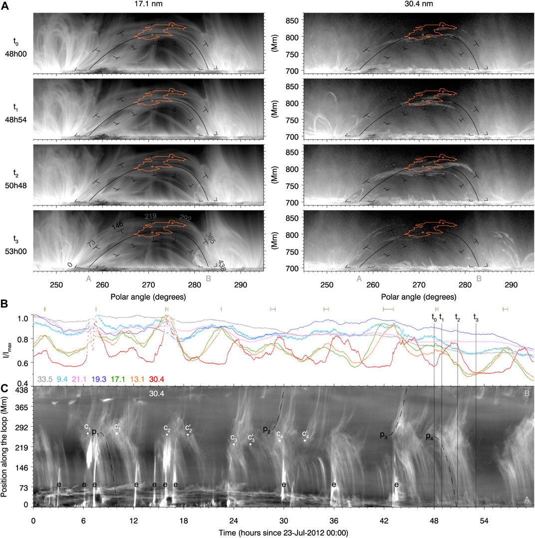
FIGURE 7. Summary figure for the “rain bow” event of Auchère et al. (2018) (Figure 6 © AAS. Reproduced with permission). (A) illustrate the temporal evolution of the transequatorial loops studied in the 171 Å and 304 Å passbands of SDO/AIA. (B) shows the light curves in seven channels of SDO/AIA. These light curves are averaged over the orange contour presented in the top pannels. (C) shows the intensity in the 304 Å channel of SDO/AIA, along the bundle of loops as a function of time. Periodic rain showers are seen in phase with the EUV pulsations. For details see Auchère et al. (2018).

FIGURE 8

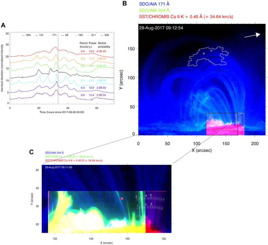
FIGURE 8. Detection of long-period intensity pulsations and coronal rain in the same loop bundle. (A) EUV light curves in seven spectral bands of the SDO/AIA. There is significant Fourier power in most spectral bands. These light curves are averaged over the white contour near the loop apex of the right panel. (B) RGB image combining two spectral bands of SDO/AIA and Ca II K observations from the SST/CHROMIS. (C) Zoom on the coronal rain observed with the SST instruments. All these figures are adapted from Froment et al. (2020) (Figures 2, 4, 7, reproduced with permission © ESO. ).

Unlike in Auchère et al. (2018), Froment et al. (2020), the main case of long-period intensity pulsations presented in Froment et al. (2015) showed little to no coronal rain as it was re-examined off-limb (but unpublished) with observations of the extreme Ultraviolet Imager (EUVI; Wuelser et al., 2004) from the Sun Earth Connection Coronal and Heliospheric Investigation instrument suite (SECCHI; Howard et al., 2008) onboard the Solar Terrestrial Relations Observatory (STEREO; Driesman et al., 2008; Kaiser et al., 2008). Such cases may be the manifestation of incomplete condensation events (Mikić et al., 2013), as discussed in Section 2.1.1, but it remains to be properly investigated.

2.2.2 Prominences and Coronal Rain

Prominences, as the name entails, are by far the most famous phenomenon on the “cold” side of the solar corona. Since the 1950s, thermal instability has been suggested as one of the dominant mechanisms for these structures (Parker, 1953). Another main requisite for prominence formation has been a magnetic topology favourable for sustaining the plasma in the corona, such as very long (mostly) horizontal field, or dipped field (Vial and Engvold, 2015). However, this requirement was relaxed through the discovery of TNE (Karpen et al., 2001), which was then applied as a model for prominences, through an evaporation-condensation cycle, perhaps with the additional help of magnetic dips. Observational support for this kind of prominence formation has been provided by Liu et al. (2012). Incidentally, this laid the foundations for the understanding of coronal rain as a separate phenomenon to prominences that does not rely on magnetic support for its occurrence.

Three kinds of coronal rain have been observed so far:

• Quiescent coronal rain

• Flare-driven coronal rain

• Hybrid prominence/coronal rain

The quiescent coronal rain kind is by far the most studied and common, and the observed coronal rain properties largely refer to this kind. However, setting the different origins of these coronal rain kinds aside, properties such as the thermodynamics, morphology and kinematics seem to be largely the same. For this reason, we present at large the various coronal rain properties within the quiescent coronal rain section below, and only denote the differences with the other two when it applies. A discussion of these results in the wider context of coronal heating and other major fields of research is presented in section 3.2.

2.2.3 Quiescent Coronal Rain

In section 2.2.1 we saw the link between coronal rain and TNE. Here we will focus on the observed local properties of coronal rain. That is, its thermodynamics, morphology and kinematics. The main character of this phenomenon, and the reason behind its name, is the downward motion along loop-like trajectories combined with its clumpy character. So much so, that other names associated with it include “blobs,” “clumps,” “droplets,” “snowflakes (in the oven),” “showers” and ‘loop prominences’. Some reports also mix in the same category the post-eruptive prominence fall-back. We do not encourage this association given the very different origin.

Coronal rain observations go back several decades, to Kawaguchi (1970), Leroy (1972) and likely further back, as seen in the NCAAR archive from the 1950s, where it was referred as “loop prominences” and thus not properly distinguished from the prominence phenomenon. With the advent of high resolution observations, and in particular with Hinode, SST and IRIS, a breakthrough was made in the understanding of this phenomenon. The currently accepted definition of coronal rain is that of partially ionised, clumpy material produced in the solar corona appearing in a timescale of minutes in transition region or chromospheric lines and falling back towards the solar surface along loop-like trajectories (see Figure 9). The temperatures and densities associated with it are, respectively, 10⁴–10⁵ K, and 10¹⁰–10¹² cm⁻³ on average. In addition, EUV emission is also associated with it, due to the Corona Condensation Transition Region (CCTR), in analogy to the PCTR for prominences. Because of its coronal occurrence, this phenomenon therefore gathers coronal, transition region and chromospheric properties all together, thereby making it extremely rich in physical processes.

FIGURE 9

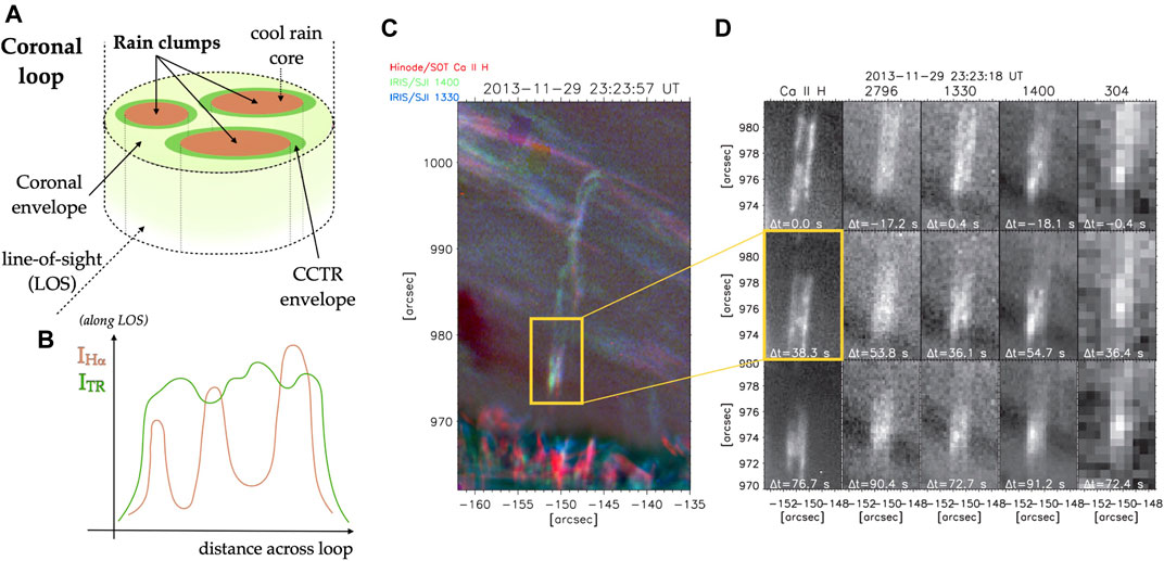
FIGURE 9. Morphology of a rain clump and a shower. (A) Sketch of a 3D cross-section of a coronal loop with coronal rain. The cool cores are surrounded by the CCTR (condensation corona transition region), a thin envelope of warmer material at transition region temperatures, which is itself surrounded by coronal plasma. (B) the emerging intensity in chromospheric (orange, e.g., Hα) and transition region (TR) lines when observing the loop along the sideways LOS, as indicated on the left. The sketches are taken from Antolin (2020) (Figure 2). (C) A shower event observed with Hinode/SOT in Ca II H (in red, T ≈ 10⁴ K), IRIS/SJI 1330 (in blue, T ≈ 10^4.3 K) and IRIS/SJI 1400 (in green, T ≈ 10^4.8 K). (D) Zooming onto the head of the shower, various clumps and a strand-like structure (aligned with the flow of the rain) can be seen. From (A–D), the panels are placed in order of increasing temperature formation (with IRIS/SJI 2796 at T ≈ 10⁴ K and AIA/304 at T ≈ 10⁵ K), and from (A, B) at 3 consecutive instances in time (the snapshots closest in time to SOT are chosen for each instrument). For more details see Antolin et al. (2015) (adapted from Figures 10, 11 of that paper, © AAS. Reproduced with permission).

2.2.3.1 Temperatures and Spectral Features

The quiescent kind of coronal rain is linked to active region coronal loops and seems to be the most common kind of rain at times of high solar activity. Multi-wavelength observations combining AIA and another instrument probing the cool temperature range such as IRIS, SST or NST clearly show that coronal rain corresponds to a catastrophic cooling phenomenon in loops (Ahn et al., 2014; Antolin et al., 2015; Kohutova and Verwichte, 2016). Accordingly, as explained in section 2.2.1, a timelag in emission is seen from hotter to cooler passbands (Froment et al., 2020). However, during the formation of coronal rain and throughout its lifetime, emission from EUV, UV and visible wavelengths is common, indicating multi-thermal and strongly inhomogeneous fine-scale structure.

On the low temperature end, estimates have been obtained based on spectral line widths in Hα, Ca II H and Ca II 8542 (Antolin and Rouppe van der Voort, 2012; Antolin et al., 2012), where average temperatures oscillate between 5000 K and 33 000 K, with minima of 2000 K or less (Antolin et al., 2015). Observing with multiple lines simultaneously offers the possibility of more precise temperature measurements, along with non-thermal broadening estimates (see Figure 10), by assuming a common temperature and non-thermal line broadening between lines forming in similar conditions (Ahn et al., 2014; Froment et al., 2020; Kriginsky et al., 2021). The reported non-thermal broadening average values oscillate between 6 and 12 km s⁻¹, with maxima of 20 km s⁻¹. These values are particularly important for coronal heating, since they provide upper estimates for the turbulence in thermally unstable coronal loops. The optical thickness has also been estimated using the cloud model (Beckers, 1964), with values of 0.5–1.5 for Hα and 0.1–0.3 for Ca II 8542 (Ahn et al., 2014). Interestingly, while progressive cooling was found in Antolin et al. (2015), with lower temperatures at lower heights, an opposite trend was found in (Ahn et al., 2014). These trends may be anti-correlated with velocity, with higher final velocity (110 km s⁻¹) for the cooler rain (while 80 km s⁻¹ was reported for the warmer rain), which may reflect an effect from the compression downstream.

FIGURE 10

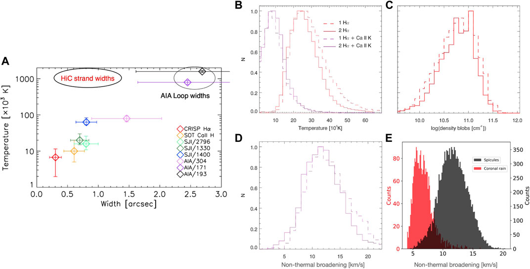
FIGURE 10. Statistics of rain widths and thermodynamic properties. (A) measured widths of coronal rain clumps with respect to the measured temperature, as observed in different lines from various instruments (each with different colour, see legend in the panel) by Antolin et al. (2015) (adapted from Figure 17, © AAS. Reproduced with permission). The AIA loop widths hosting the clumps are shown. In addition, we add the region corresponding to the Hi-C strands (Williams et al., 2020). Right, 4-panel: Temperatures [(B), in units of 10³ K], Densities [(C), cm⁻³] and Non-thermal broadening [(D), km/s] of rain clumps observed in Froment et al. (2020) with the SST/CRISP (in Hα) and CHROMIS (in Ca II K) instruments (from Figures 12 and 15 of that paper, reproduced with permission © ESO). Non-thermal broadening [(E), km/s] observed in Kriginsky et al. (2021) with SST/CRISP (in Hα) and CHROMIS (in Ca II 8542) (from Figure 7 that paper, reproduced with permission © ESO). In panel (E) a comparison with measurements for spicules seen in the same FOV is included.

Claes and Keppens (2019) indicate growth rates of minutes under coronal conditions, reflecting the exponential growth of the thermal mode in the linear stage. Similarly, when taking the wave-caused perturbation of the heating function into account, Kolotkov et al. (2020) show that the growth (or damping) times of the acoustic and thermal modes in typical coronal conditions can vary from several minutes to several tens of minutes. This suggests that a single rain clump, without any additional effect than its cooling, should exhibit the intermediate TR temperatures of the cooling range for only a very short duration. The fact that we see continuously multi-thermal emission for single clumps at high resolution suggests a more complex structure in which a clump is surrounded by a warm shell at TR temperatures, which itself is in contact with the ambient coronal plasma (Antolin, 2020). This shell corresponds to the CCTR, and is observed to be very thin, under the 0′′.33 resolution of IRIS (Figure 9), in agreement with 1D modelling results Xia et al. (2011). Furthermore, this UV and EUV emitting shell is expected to be more extended than the chromospheric emission in the longitudinal direction with respect to the magnetic field, also supported by observations (Ahn et al., 2014; Antolin et al., 2015; Vashalomidze et al., 2015). This is because the rain produces strong compression downstream, particularly prior to impact with the chromosphere, which then increases both the density and temperature (Müller et al., 2003, 2004). The shell is also expected to extend along the wake of the rain due to flux-freezing conditions. In addition, the inhomogeneous character of the rain means that highly localised high density regions are produced, as shown in multi-dimensional simulations (Fang et al., 2015). As we will see below, this leads to a differential longitudinal velocity with denser clumps falling faster than lighter clumps, leading to V-shape structure in 2D where the head is denser than the tail, thereby further extending the UV and EUV emission along the rain’s path.

2.2.3.2 Densities

Coronal rain densities between 2 × 10¹⁰ and 2.5 × 10¹¹ cm⁻³ have been determined through EUV absorption (Antolin et al., 2015), assuming that the EUV emission from the rain clumps themselves is negligible and assuming ionisation equilibrium. Given the very thin CCTR shell, the former assumption should hold as long as most of the EUV emission observed comes from the region upstream or downstream of the dense part of the rain. Also, these number densities correspond to the neutral H, He and singly ionised He, which are the elements causing the continuum absorption. Electron number densities can be inferred assuming an ionisation fraction for the rain. A word of caution here is that ionisation equilibrium is likely not to hold, given that rain clumps are cooling rapidly, likely on similar timescales as recombination and ionisation, and it is unclear if heating (either through an unknown coronal heating source of through downstream compression or shear flows) prevents further cooling. For instance, temperatures as low as 2000 K have been measured in coronal rain (Antolin et al., 2015). However, the energy released through the recombination process should slow down the cooling rate (Ballester et al., 2018), which has found observational support (Antolin et al., 2015). The very fast cooling timescales combined with heating mechanisms produced by the flows and the short lifetime of the rain clumps makes the ionisation degree of coronal rain uncertain, but very likely much higher than for the prominence case. Further work is necessary to properly determine the ionisation degree in coronal rain, and properly assess the assumption of ionisation equilibrium.

Another, more robust electron number density estimation method for coronal rain is provided by Gouttebroze et al. (1993), and applied in Froment et al. (2020) to find average values of (6.7–8) × 10¹⁰ cm⁻³ with maxima at 10¹² cm⁻³, similar to the EUV absorption values stated above (see Figure 10). This method relies on the good correlation between absolute intensity in Hα and the emission measure $EM={\int }_0^D{n}_e^{2}dz$, where D denotes the thickness along the LOS of a rain clump and n_e is the electron number density. This relation is based on the dominance of photoionisation in the Lyman continuum and scattering of the incident radiation from the solar disk.

2.2.3.3 Dynamics

Regarding the dynamics of coronal rain clumps, they are characterised by their average downward velocities. Spectroscopic high-resolution observations have allowed to determine the distribution of total velocities, taking into account the plane-of-the-sky and Doppler components (Antolin and Rouppe van der Voort, 2012; Antolin et al., 2012; Ahn et al., 2014; Froment et al., 2020), leading to average total velocities of (30–50) km s⁻¹ at the loop apex and (80–100) km s⁻¹ towards the footpoints, with a long tail towards higher velocities of 200 km s⁻¹ or so (Kleint et al., 2014; Schad et al., 2016). It has been known for several decades that other forces besides gravity must be present in order to observe the lower than free-fall accelerations. Indeed, early observations with TRACE and EIT have shown that downward accelerations are about a third of the solar gravity value (Schrijver, 2001; De Groof et al., 2004), and about a half of what is expected from the effective gravity along an elliptical loop (Antolin and Verwichte, 2011; Antolin and Rouppe van der Voort, 2012). Gas pressure forces have been shown to play a major role (Mackay and Galsgaard, 2001), leading to deceleration and even reversal of the direction of the rain (Antolin et al., 2010; Kohutova and Verwichte, 2017a). In 1D simulations of fully and partially ionised plasma Oliver et al. (2014), Oliver et al. (2016) have shown that the formation of a condensation produces a restructuring of the gas pressure downstream, which ultimately leads to constant downward velocities that are indeed sometimes observed (Antolin et al., 2010). On a timescale determined by the sound speed, the clump stops accelerating and the final speed is found to be determined by the density with a well-defined power law of ≈ ρ^0.64. This process has been shown to hold in 2D for magnetic fields above 10 G (Martínez-Gómez et al., 2020), shown in Figure 11. For large magnetic field values, the downstream compression produced by the clumps leads to expansion of the field lines, which lead to an upward magnetic tension that further decelerates the rain (Kohutova and Verwichte, 2017a). A combined gas pressure and magnetic tension force must therefore be at the origin of this striking relation. It is unclear, however, how much does this relation apply to the complex solar atmosphere. The very fast speeds of the rain prior to impact suggest that this physical process may not be dominant. In a large statistical survey of supersonic downflows observed with IRIS, Samanta et al. (2018) find that those with a chromospheric component are 10 km s⁻¹ faster, which may find an explanation in this effect (see Figure 16).

FIGURE 11

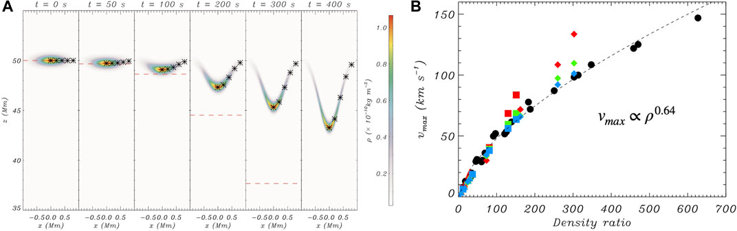
FIGURE 11. Simulated downward motion of a rain-like clump. (A) Snapshots of density at different times of a clump falling under the action of gravity in a homogeneous atmosphere in a 2.5D MHD setup. The dashed red line denotes the position that would correspond to a free-falling object. (B) the maximum velocity achieved by the clump plotted against the density ratio Θ between the clump and the external environment. Different colours denote simulations with different magnetic fields. Red, green and blue colour correspond to B₀ = 5, 10 and 20 G, respectively. Triangles, squares and diamonds denote different maximum clump densities, with 1, 5, 10 × 10^{–10 kg} m⁻³, respectively. The dashed curve shows the fit v_max = 2.56Θ^0.64, with Θ the density ratio (taken from Figures 1, 3 in Martínez-Gómez et al., 2020, reproduced with permission © ESO.).

As suggested above, the fact that a variety of dynamics are observed, including very fast speeds close to free-fall indicate that many other factors are at play, among which magnetic forces. Transverse MHD waves are often observed in coronal loops, which can be particularly well traced for coronal loops with rain thanks to the higher resolution available when observing in cool UV or visible lines (Antolin and Verwichte, 2011; Kohutova and Verwichte, 2016). It was therefore speculated that the ponderomotive force could have an effect, acting on rain clumps as beads on an oscillating string (see Figure 19). This was analysed with a one-dimensional analytical model by Verwichte et al. (2017), in which it was shown that the loop behaves like a dynamical system with stable points (locations where rain can be stopped) and unstable points (such as saddle points, that prevent the accumulation of rain). In the analysis of Verwichte et al. (2017), 2 cases were considered depending on the rain’s mass being significant with respect to the loop’s initial mass. In the case of little rain, the analysis applies to individual clumps, and it was shown that the acceleration from the ponderomotive force preventing a clump from falling needs to satisfy:

$a>a_{\text{crit}}=\frac{\sqrt{2g_{◦}R}}{v_{A}n},(16)$

where n refers to the longitudinal harmonic and needs to be odd for holding a clump at the loop apex, R is the loop radius (assuming a semi-circular loop) and v_A denotes the Alfvén speed. Taking typical coronal values of R = 50 Mm, v_A = 1,000 km s⁻¹, yields a_crit = 0.17/n, corresponding to a displacement of 8/n Mm. Such amplitudes are large for usual transverse oscillations in active regions (Anfinogentov et al., 2015), but are observed for external perturbations such as eruptions. The analysis was applied to a specific database and shown to explain successfully the observed rain kinematics. However, on average, the ponderomotive force from transverse MHD waves was found to be insufficient to fully explain the observed reduced downward velocities.

Another interesting consequence of coronal rain is the excitation of transverse oscillations, particularly targeting the large rain events or “showers” (described further below) for which the mass fraction is large relative to the initial loop mass. Verwichte et al. (2017) show that the transverse displacement is approximately linearly proportional to the ratio m/M, of rain mass m relative to the loop’s mass M, and is expected to be on the order of several hundred km, matching observations. This scenario is further supported by 2.5D MHD simulations by Kohutova and Verwichte (2017b), where the process is found to be characterised by a decrease of the oscillation period as the rain falls down the loop. This mechanism could therefore be partly responsible for the observed decay-less small-amplitude transverse oscillations (Nisticò et al., 2013; Anfinogentov et al., 2015), whose periods are found to be correlated with the loop length (Nechaeva et al., 2019). Although in this scenario the coronal rain excites primarily the fundamental mode, the fact that the period changes with time due to the varying temperature and density, would lead to scatter in the period-length correlation, which may or may not agree with observations. This mechanism is particularly interesting when parameters such as the loop inclination, the clump’s location, speed and displacement can be well determined, since it provides a seismological method. This has been successfully applied in Verwichte and Kohutova (2017), where it is found that the rain comprises two thirds of the loop mass.

Further seismological applications are presented by the longitudinal oscillations of the rain, produced by the combination of gas pressure and magnetic forces (Kohutova and Verwichte, 2017a). When the cool material is far from the footpoint, the dynamics are governed by the gas pressure and gravity, and the system presents a series of stable and unstable points, of particular interest for prominence formation. This has been recently explored by Adrover-González et al. (2021).

2.2.3.4 Morphology

Coronal morphology varies greatly according to wavelength and spatial resolution. As explained above, coronal rain is multi-thermal, and the cold and dense core surrounded by thin but elongated warm sheath at transition region temperatures means that the clumpy character is particularly appreciated in chromospheric wavelengths such as Hα or Ca II H. Accordingly, the widths are sharply distributed at these temperatures around a few hundred km on average, with, however, an abrupt drop at the lower end that suggests limitations from spatial resolution (see Figure 10). Observations with the SST with $\approx 100$ km resolution lead to averages of 200–300 km, with minima and maxima around 150 and 500 km (Antolin and Rouppe van der Voort, 2012; Froment et al., 2020), while the flare-driven rain observed in Hα at higher resolution with the NST ($\approx 40$km), exhibits averages of 120 km, with minima/maxima of 70/250 km (Jing et al., 2016). It is therefore possible that the currently resolved structure is a tip-of-the-iceberg distribution, with far more clumps at higher resolution (Scullion et al., 2014). This is supported by 2.5D simulations by Fang et al. (2013), Li et al. (2022), where a sharp increase in numbers for blob sizes of 50–100 km is obtained. Further support can be found in observations, by noting the stark increase in width values with observations in the SJI 2796 passband with IRIS at $\approx 240$km resolution, dominated by the Mg II k line at similar formations temperatures than Hα (Antolin et al., 2015). Indeed, the Mg II k rain clumps appear with widths of 580 km, with minima/maxima of 300/900 km.

The clumpy morphology is accompanied by a peculiar multi-stranded structure that is particularly visible at high resolution in chromospheric lines (Antolin et al., 2015; Froment et al., 2020). While the clumpy morphology is well-reproduced by multi-dimensional simulations, and the shear flows produced by TI naturally lead to a strand morphology, it is unclear whether the observed multi-stranded structure is well reproduced. Indeed, the strands obtained through the shear flow process are 1–2 Mm apart (see Figure 12), while the observed strands are just a few hundred km apart, extending in the transverse direction for up to 3 Mm (Antolin et al., 2015). It was then hypothesised that TI may be generating this structure through a perpendicular thermal conduction effect (van der Linden and Goossens, 1991).

FIGURE 12

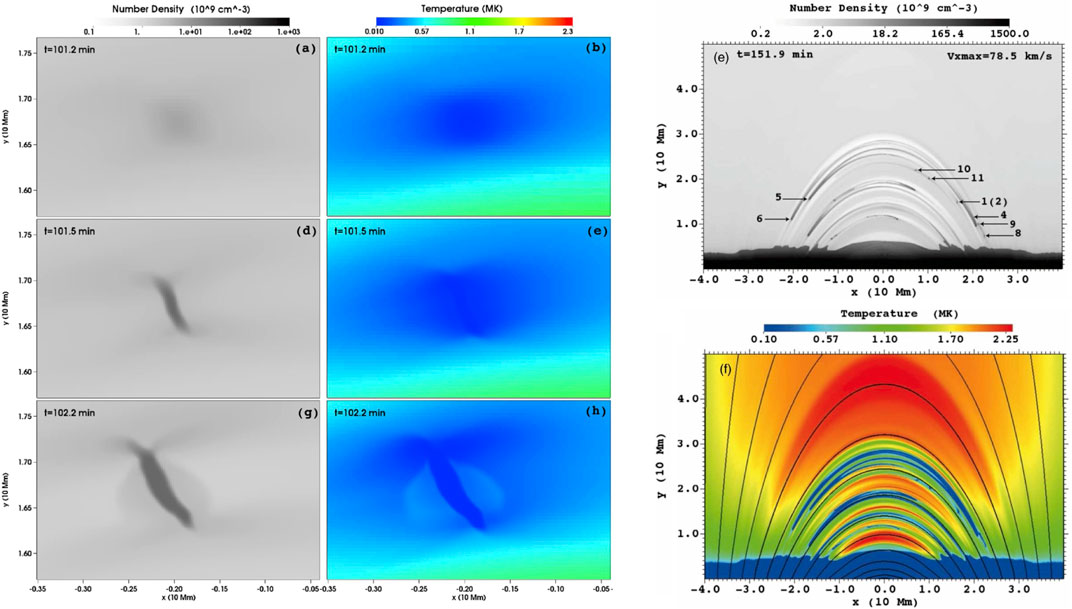
FIGURE 12. 2.5D MHD modelling of coronal rain. Left: zoomed-in region of $\approx 3\times 2$ Mm² focusing on the formation of a coronal rain clump within a loop arcade (shown on the right) as shown by Fang et al. (2015). Note that the clump first forms in the direction transverse to the field and grows over a distance of $\approx 1$ Mm within 1 min. The number density and temperature maps are provided. Right: the advanced stage of the same simulation, shown in Fang et al. (2013), where several elongated (V-shape) clumps can be seen (top and bottom panels show, respectively, number density and temperature). Adapted from Figures 1, 2 in the respective papers (© AAS. Reproduced with permission).

It is good to note, however, that opacity may also greatly influence the morphology. This is supported by observations with the Solar Optical Telescope (SOT, Suematsu et al., 2008) on board Hinode at $\approx 150$ km resolution in the Ca II H line, or with observations with CHROMIS (Löfdahl et al., 2021) at the SST (albeit with average seeing conditions) (Antolin et al., 2015). Despite the high spatial resolution of $\approx 150$ km, the Ca II H widths are 430 km on average, with minima/maxima of 150/700 km.

In contrast with the widths, the lengths of rain clumps are more sparsely distributed, with averages between 1,000–3,000 km but long tails to even tens of thousands of km (Antolin et al., 2015). This is expected given the various effects leading to clump elongation, such as shear flows (Fang et al., 2015; Li et al., 2022) and density-regulated downward velocities (Oliver et al., 2014; Martínez-Gómez et al., 2020).

2.2.3.5 Showers

A peculiar property of coronal rain is the fact that rain clumps falling along a similar trajectory appear quasi-simultaneously over a relatively wide region (Antolin and Rouppe van der Voort, 2012). This coherency has a transverse length scale of a few Mm (with respect to the flow of the rain, assumed to be the direction of the magnetic field), and is observed in both large loop systems or relatively isolated loops (Şahin and Antolin, 2022, manuscript in preparation). This is about an order of magnitude larger than a cool and dense clump width (see Figure 9). The timescale of this synchronous behaviour seems to be on the order of minutes or less. This rules out a random behaviour or solely TNE in different field lines without transverse communication. Indeed, if the latter, assuming common footpoint heating conditions and therefore approximately similar TNE cycles across neighboring field lines, would yield an apparent expansion effect in which the rain is seen in gradually longer and higher loops, which is not observed for quiescent rain.

Multi-dimensional simulations by Fang et al. (2013, 2015) have provided a clue behind this behaviour (see also Li et al., 2022). Indeed, a region composed of loops exposed to the same heating function and thus differentiating themselves only on the length, exhibit thermal instability leading to coronal rain quasi-simultaneously, a behaviour denoted as “sympathetic cooling” (see Figure 12). The growth of the unstable region in the direction perpendicular to the loop occurs on a timescale of a minute or so. The physical mechanism behind this is the trigger of the thermal instability in neighboring field lines due to the slow and fast mode perturbations produced by the first TI at the centre of the loop system. In a 3D MHD simulation encompassing a large loop system Moschou et al. (2015), Xia et al. (2017) have confirmed this behaviour, adding the fact that the locations of condensations also coincide with locations unstable to the convective continuum instability (CCI), leading to interchange mode or Rayleigh-Taylor type instabilities at the apex of the loop. However, it is important to note that the coronal magnetic field in these simulations is more of a Quiet Sun type (a few Gauss), and it is therefore unclear whether the CCI would also be effective in active regions. More recently, Jenkins and Keppens (2021) have shown that CCI precedes TI in flux rope configurations, and therefore may play a role in the formation of condensations and showers. In any case, these simulations suggest that showers may be a clear signature of TI within TNE cycles in the sense that TI acts as a locking/syncing mechanism across field lines that are only critically stable. In that sense, the observed few Mm transverse coherency length is produced by a combination of similar footpoint heating conditions across the different field lines and the cross-field effects associated with TI.

While 3D MHD simulations can reproduce to some extent relatively large-scale structures such as showers, they cannot reproduce small observed clumps, due to the limited resolution achieved in the corona (a necessary sacrifice to allow high resolution in the lower atmosphere in non-adaptive codes). They neither can reproduce the high magnetic Reynolds of the corona, meaning that important effects are likely missing. However, these simulations can shed light into the formation process of coronal rain in more realistic atmospheres. Recently, Kohutova et al. (2020) reported for the first time coronal rain generated self-consistently in a 3D radiative MHD simulation with the Bifrost code (see Figure 13). The heating in Bifrost is dominated by Ohmic dissipation (Kanella and Gudiksen, 2019). The heating per unit mass exhibits an apex to footpoint ratio of about 0.1. Also, as seen in Figure 13, the loop with coronal rain experiences high frequency heating, with a few large heating events with durations on the order of 100–200 s. This matches the theoretical conditions for TNE.

FIGURE 13

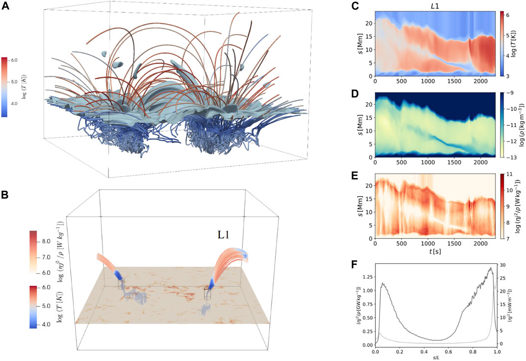
FIGURE 13. Self-consistent coronal rain formation in a 3D RMHD simulation with Bifrost, by Kohutova et al. (2020) (Figures 1, 3, 4, 7 reproduced with permission © ESO). (A) 3D configuration of the simulation domain (24 × 24 × 16.8 Mm), visualising magnetic field lines. The colour denotes the temperature. The 5 × 10^{–12 kg} m⁻³ density isosurface is shown in blue. Several cool and dense condensations can be seen in the c orona. (B) A snapshot of selected magnetic field lines crossing a condensation in a loop marked L1. The colour denotes the temperature. The surface at z = 1.2 Mm shows concentrations of strong Joule heating in the chromosphere. The loop footpoints are outlined by a black surface. Top 3-panel on the right: (C–E) Evolution of temperature, density and Joule heating per unit mass along a selected field line of loop L1 crossing the condensation. (F) Time-averaged Joule heating per unit mass (solid) and volumetric heating (dotted) along loop L1, normalised by loop length. See Kohutova et al. (2020) for further details.

Because of their larger widths and lengths, showers can often produce clear EUV absorption features (Antolin et al., 2015). An extreme example of a shower is the flare-driven rain, resulting from the simultaneous and similar heating to a group of field lines during the reconnection event in the corona. Accordingly, dark EUV flaring loops, also known as “Dark Post-Flare Loops” (Song et al., 2016), can be explained by the shower mechanism, as shown by Ruan et al. (2021).

2.2.4 Flare-Driven Coronal Rain

Coronal rain is observed primarily in active regions and is usually termed as “quiescent”. However, the most striking appearance of coronal rain occurs in flaring loops, during the gradual phase of a flare (see Figures 14, 17). Although statistics await, flare-driven coronal rain seems to be an integral component of flare evolution (Foukal, 1978; Tandberg-Hanssen, 1995). It may play a role in the phenomenon of quasi-periodic pulsations strongly associated with flares, for which thermal effects are deemed important (Zimovets et al., 2021). Moreover, the amount of coronal rain observed seems strongly correlated to flare intensity and duration. Despite this very strong presence, flare-driven rain remains largely unstudied. Based on observations, the rain bears strong similarities with the quiescent kind in terms of morphology and dynamics as observed in Hα, being clumpy and multi-stranded with a few hundred km widths, a factor of 10 larger lengths and downward velocities on the order of 100 km s⁻¹ (Jing et al., 2016; Scullion et al., 2016; Kuridze et al., 2019). Another parallel is the observed multi-thermal nature of the rain. On the other hand, an important difference is the increased density, with common values in large flares of 10¹²–10¹³ cm⁻³, as estimated from white light continuum due to Paschen and Brackett recombination (Jejčič et al., 2018) or Thomson scattering (Martínez Oliveros et al., 2014; Saint-Hilaire et al., 2014), further supported by non-LTE inversions of Ca II 8542 and Hβ lines (Koza et al., 2019). A further interesting difference is the observed large non-thermal line broadening in chromospheric lines (Lacatus et al., 2017), consistent with the expected increase in turbulence (Kontar et al., 2017).

FIGURE 14

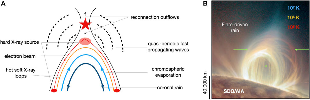
FIGURE 14. Flare-driven coronal rain and its place in the standard flare model. (A) Sketch of the standard flare model, with the reconnection region depicted as a red star in the corona. Several of the usually observed processes during a flare are indicated. (B) M7.7 class flare observed by SDO/AIA on 19 July 2012, on the West limb of the Sun. The composite image shows AIA/94 in blue (10⁷ K), AIA/171 (10⁶ K) and AIA/304 (10⁵ K) in the gradual phase of the flare, where coronal rain (indicated by green arrows) can be observed tracing a dome-like structure.

Early studies recognise the role of thermal instability in the formation of condensations during the cooling of a flaring arcade (Goldsmith, 1971; Antiochos, 1980). The instability onset can be understood in terms of the following timescales, the conductive cooling time τ_cond at high flaring temperatures T_h = 10⁷ K and pressures p_h = 80 dyn cm⁻², the radiative cooling time at 10⁶ K, τ_rad (taking the radiative loss function as ΛT^α, with Λ = 10^–21.31 and α = 0, Colgan et al., 2008), and the free-fall time along the loop with apex height H = 5 × 10⁹ cm:

$\begin{array}{ccc}\hfill \text{i}){\tau }_{\text{cond}}& =\hfill & \frac{(3/2)p_h{H}^2}{10^{-6}{T}_h^{7/2}}\approx 10^3\left(\frac{p_h}{80}\right){\left(\frac{H}{5\times 10^9}\right)}^2{\left(\frac{10^7}{T_h}\right)}^{7/2}\text{s}\hfill \end{array}(17)$

$\begin{array}{ccc}\hfill \text{ii}){\tau }_{\text{rad}}& =\hfill & \frac{(3/2)p}{n^2\mathrm{\Lambda }}\approx 30\left(\frac{3\times 10^{10}}{n}\right)\left(\frac{T}{10^6}\right)\text{s}\hfill \end{array}(18)$

$\begin{array}{ccc}\hfill \text{iii}){\tau }_{\text{ff}}& =\hfill & {\left(\frac{2H}{g_{◦}}\right)}^{1/2}\approx 600{\left(\frac{H}{5\times 10^9}\right)}^{0.5}\text{s},\hfill \end{array}(19)$

where we assume an electron number density of n = 3 × 10¹⁰ cm⁻³, common for flaring loops. It is clear that once conduction cooling drops, the fact that τ_rad < τ_ff allows the possibility of TI to take place. This, however, crucially depends on the shape of the temperature profile in the corona, as shown by Antiochos (1980). Indeed, a profile produced by thermal conduction, with maximum temperature at the apex does not lead to TI, while profiles that are flat or temperature dipped (even with only 5%) are enough to trigger TI and the formation of condensations. This result lead (Antiochos, 1980) to hypothesise on the existence of a long-lived heating mechanism during flares, concentrated at the loop footpoints, so as to produce such flat-shaped temperature profiles that would lead to coronal rain. It is then important to question what temperature profiles along a loop are realistic for a cooling flaring loop.

Recently, Reep et al. (2020) conducted a parameter study of flaring loops with HYDRAD, assuming the electron beam as the main energy input (and the accompanying thermal conduction). Parameters such as the energy flux of the beam, the low-energy cut-off, the duration and left-right asymmetry were varied, along with loop length. In no case condensations were observed, agreeing with Antiochos (1980) on the fact that such loops have all a temperature profile with maximum at the apex. The short-lived nature of the electron beam, combined with the fact that, if long-lived, the location of its deposition shifts rapidly from the footpoint towards the apex, ensures uniformly heated loops at all times during their cooling.

Besides a secondary source of heating, other possibilities for flare-driven rain formation include multi-dimensional effects, such as an additional magnetic pressure at the apex produced by the reconnection jets above (Takasao and Shibata, 2016). Such additional pressure leads to larger apex densities and more slow mode shocks, which could more readily trigger TI. Recently, realistic global 3D MHD simulations that include flux emergence manage to produce flare-like large energetic release events, with coronal rain formation successfully reproduced (Cheung et al., 2019; Chen et al., 2021). Such simulations do not include particle acceleration and therefore suggest the possibility of thermal conduction combined with multi-dimensional effects as mainly responsible for flare-driven rain, and may also question how important the electron beam is in the flare process. This has been recently supported by the first 2.5D flare simulation including a realistic treatment of particle beam heating (Ruan et al., 2021). Indeed, the electron beam is found to be unimportant with respect to thermal conduction, while a reduction of the loop area post reconnection is suggested to play a role in the trigger of TI. However, the simulated flare is only of B class, and therefore it is yet unclear how the electron beam, thermal conduction and multi-dimensional effects combine in generating the rain. It is worth to note that recent observations have shown that some flares can be mainly powered by thermal conduction (López et al., 2022).

2.2.5 Hybrid Prominence/Coronal Rain

Besides the flare-driven coronal rain there is a recent kind of coronal rain whose origin is more directly linked to the magnetic topology. In particular, this kind relies on magnetic support so that horizontal field (or very long loops) and magnetic dips seem necessary for its existence (see Figure 15). Such coronal rain is seen both in active regions and in the quiet Sun, and can involve open field regions. Because of the characteristics in terms of dynamics, morphology and duration, this coronal rain type resembles prominences, and in particular quiescent prominences. We therefore refer to it as “hybrid prominence/coronal rain” (Liu et al., 2016)².

FIGURE 15

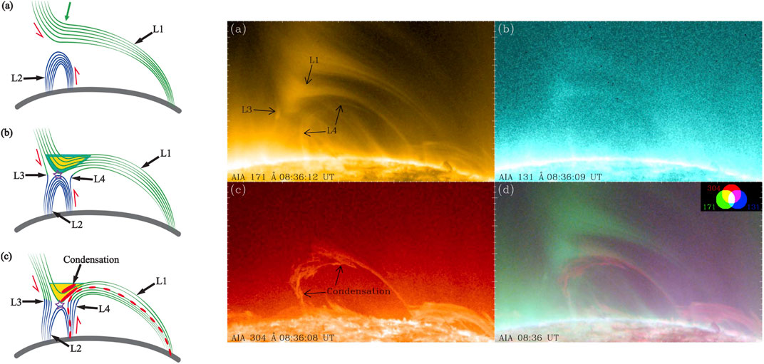
FIGURE 15. Hybrid prominence/coronal rain structure. Left: A sketch of the structure. Magnetic field lines in green (L1) form a dip where plasma can settle and catastrophically cool to form condensations. The material can spill down along L1 as coronal rain. Magnetic reconnection can take place with coronal loops below (L2), case in which the cool material can slip through and fall as coronal rain. New sets of loops (L3 and L4) form through reconnection, and can also carry with them part of the condensed material. The green lines (L1) can be open or closed. If open, then the reconnection is of an interchange type. Right: A 4-panel figure showing, from top to bottom and left to right, AIA/171, AIA/131, AIA/304 and a composite image of all 3. An X-type structure can be seen, in which the cool material (seen in 304) accummulates and rains down. Both figures are adapted from Li et al. (2018) (Figures 5,6 © AAS. Reproduced with permission.).

The observations of such structures may actually be traceable several decades back, to other structures denoted as “coronal spiders” and “cloud prominences” (Dunn, 1971; Lin et al., 2006), characterised by their formation at high altitudes and peculiar shapes. More recently, combined observations with AIA and IRIS, combined with magnetic field extrapolations with HMI have allowed a clearer picture of this phenomenon, paving the way to a new category of coronal rain (Liu et al., 2016). With stereoscopic observations with both AIA and STEREO, Schad et al. (2016) have reported a catastrophic cooling event followed by coronal rain falling over several hours from a magnetic dip associated with an X-point structure, allowing magnetic field measurements (through long integration times) with FIRS (Jaeggli et al., 2010) at the Dunn Solar Telescope (DST) (see Figure 18). A similar structure and evolution has been observed by Li et al. (2018), in off-limb observations with AIA, involving both closed/open loops underneath/above an X-point, suggesting in part slippage of the dense, partially ionised plasma through the X-point. Such models are reminiscent of the forced reconnection analytical models by Low et al. (2012a,b), aimed at explaining the observed vertical motion of quiescent prominence knots. Another possibility is a more active role of magnetic reconnection in the flare generation process through entropy mode excitation at the X-point (Murawski et al., 2011). Li et al. (2018) have reported on quasi-periodic fast MHD modes propagating away from the X-point, which may further excite condensations above/below of the X-point. Interestingly, the coronal rain is observed to fall along both the closed and open field lines. Mason et al. (2019) have reported on similar structures and invoked interchange reconnection, possibly in combination with TNE, to explain the appearance of the rain in the open structures near the separatrices (see Figure 15). The TNE scenario is further supported by the fact that such events are seen to occur repeatedly over several days (Li et al., 2019, 2020). The argument by Mason et al. (2019) is based on the fact that open field lines have a pressure structure and outflow velocity that would prevent TNE from happening, hence the need for a mechanism such as interchange reconnection. In this scenario, coronal rain would be happening first in the closed field lines prior to reconnection leading to their opening. This argument is only partly supported in observations, since coronal rain is observed not only close to the separatrices but on the field lines tracing the magnetic dip much further above the X-point. Actually, the fact that there is a dip should be a sufficient condition for condensations to happen, since it allows the local accumulation of plasma, which can then gradually cool down and condense.

The scenario of magnetic dips acting as generators and reservoirs of coronal rain is further supported by long-lived supersonic downflows above sunspots, first reported by Skylab XUV, HCO OSO and HRTS (e.g., Dere, 1982; Brynildsen et al., 2001), seen as mild to strong redshifts in transition region and chromospheric lines within the same spatial resolution element. At higher resolution with IRIS, very high redshifts up to 200 km s⁻¹ associated with (E)UV bright points within umbra and occasional upflows of 50–100 km s⁻¹ were reported by Kleint et al. (2014). Such events showed very strong variability, particularly in the chromospheric Mg II k line, and were associated with footpoints of thermally unstable loops seen in AIA 304 and in SJI 1400 and 2796 passbands (see Figure 16). On the other hand, Straus et al. (2015) noted the existence of a separated, shocked high redshift component with in the O IV lines with densities typical of coronal rain but with no variability, suggesting a steady siphon-type flow. Intriguingly, such downflows were observed over hour long duration. Chitta et al. (2016), reporting on a similar event, noted that the timescale to completely drain a loop with the obtained rain mass flux is 100–1,000 s, far below the observed duration times. Supersonic downflows with similar characteristics have been reported by Ishikawa et al. (2020), Nelson et al. (2020b), Nelson et al. (2020a), often reporting on the strong variability in chromospheric lines, sometimes matched in the transition region lines. Samanta et al. (2018) have searched the first 1.5 years of IRIS data, compiling 60 rasters over sunspots and found 80% with supersonic downflows, with most rooted in the penumbra, and some in the umbra (see Figure 16). Almost half of the downflows show a chromospheric component, with Doppler shifts that are $\approx 10$km s⁻¹ higher and with stronger intensities than those without.

FIGURE 16

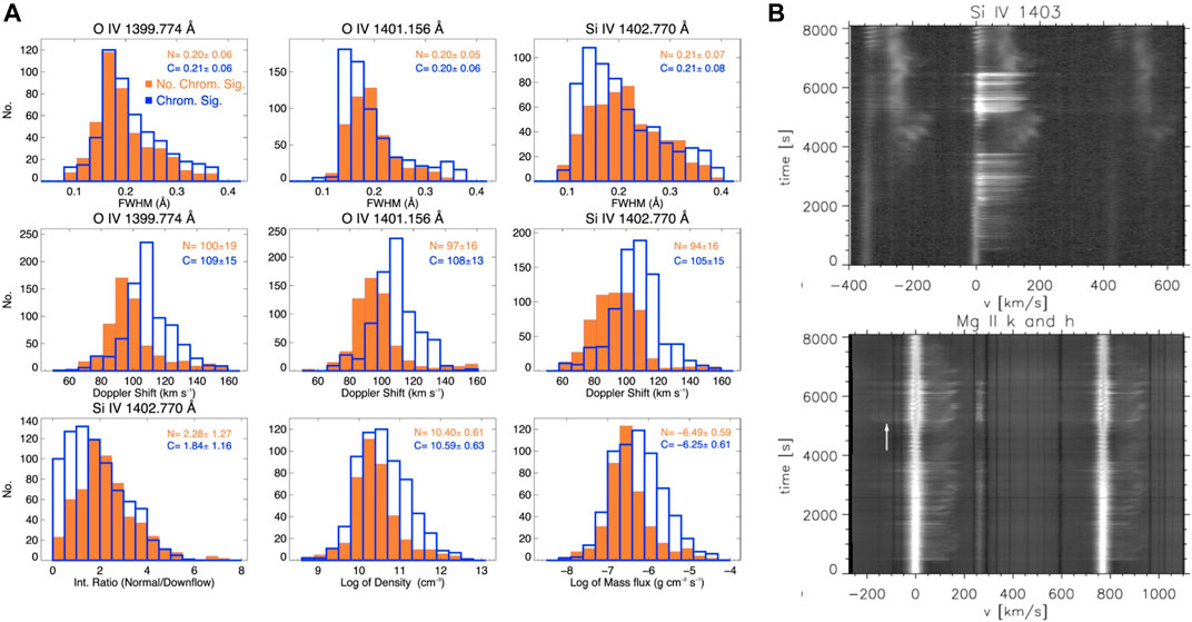
FIGURE 16. IRIS observations of supersonic downflows over active regions. (A) Statistics of observed supersonic downflows using 60 raster data from IRIS by Samanta et al. (2018) (Figure 9 of that paper © AAS. Reproduced with permission). The top and middle rows show, respectively, the FWHM and Doppler velocity distributions measured in the O IV doublet and Si IV lines. The bottom left panel shows the intensity ratio between the “normal” (background) component and the downflow (red-shifted) component in the Si IV spectra. The bottom middle and right panels show, respectively, the distribution of the densities (calculated through line ratios) and the mass flux (in log scale). In each panel the orange and blue histograms denote, respectively, downflows without and with chromospheric components. Average values with 1 σ values are printed in each panel. (B) Temporal evolution of IRIS spectra in the Si IV 1403 and O IV 1401 lines (top) and Mg II k and h lines at a bright dot within an umbra, exhibiting supersonic downflows, reported by Kleint et al. (2014) (Figure 3 of that paper © AAS. Reproduced with permission). Notice the existence of bursty (20 s timescale) and steady profiles, particularly in the Mg II and Si IV lines, respectively. Notice also the existence of simultaneous, weaker upflows (indicated by the arrow).

Although quiescent coronal rain can be considered as a siphon flow undergoing catastrophic cooling along its path, the fact that supersonic downflows are long-lived matches best with the hybrid prominence/coronal rain scenario, where a reservoir of cool material exists. The variability observed in the chromospheric passbands is often associated with the clumpy structure of the rain, and the fact that this variability is sometimes absent in transition region lines, altogether with the chromospheric component, can be attributed to a plasma that does not cool all the way down to the chromospheric regime. Such flows have been reproduced in 1D numerical simulations (Mikić et al., 2013), and are explained by the existence of strong geometric or heating asymmetries between both loop footpoints, leading to siphon flows that readily remove the plasma. In this scenario, the free-fall time τ_ff in Eq. 19 is expected to be smaller than τ_rad in Eq. 18. Recently, combining different viewpoints with SDO and STEREO, and different temperatures spanning transition region and chromospheric ranges with IRIS, Chen et al. (2022) have confirmed the link between the observed long-lived supersonic downflows and the presence of hybrid prominence/coronal rain structures providing a constant mass reservoir. They further reveal a vast network of loops (most of which are closed), involving very long prominences (among which the hybrid kind is found) connecting quiet and active regions, thereby playing an important role in the mass and energy cycle of the solar atmosphere.

3 Implications for the Mass and Energy Cycles in the Solar Atmosphere

3.1 The Delicate Coronal Mass Limit

Coronal loops are the consequence of specific heating and cooling processes taking place in the solar corona. It is generally agreed that local sources such as magnetoconvective motions at sub-photospheric level (leading to granular convection, magnetic buffeting and so forth) are largely responsible for most of the Poynting flux into the coronal volume (Parnell and De Moortel, 2012). Global sources, such as the p-mode leakage may still provide significant flux in some regions of the Sun (Morton et al., 2019). The temporal scales of the perturbations of magnetic flux structures in the lower solar atmosphere, combined with the high magnetic Reynolds nature of the plasma and the density stratification of the solar atmosphere, define the character of the energy transport. Fast perturbations with respect to the required Alfvén time for the structure to respond and adapt constitute MHD waves (AC heating). On the other hand, slow perturbations that allow the coronal structure to adapt constitute a steady build-up of magnetic stress (a field-line braiding process) that eventually is released through magnetic reconnection (DC heating). External factors such as flux emergence or mixed polarities in the lower atmosphere can also directly trigger magnetic reconnection leading to coronal heating (Chitta et al., 2017; Priest et al., 2018).

Theoretical and numerical work over the last decade have shown that the spatio-temporal properties of the energy release of these two leading coronal heating mechanisms should be significantly different, resulting in different local and global observables (De Pontieu et al., 2022). For example, Alfvén waves rely on the establishment of a turbulent cascade to efficiently dissipate their energy, which inherently implies that these waves must be able to propagate large distances, throughout the loop, to either self-interact or generate dynamic instabilities through which turbulence can occur (van Ballegooijen et al., 2011). Many Alfvén wave based models therefore predict episodic heating on very small scales, with the bulk of the heating needed to sustain a loop only achieved when integrated over length scales comparable to the pressure scale height (Matsumoto, 2018). Although subject to specific conditions, on average, this heating may lead to uniformly heated loops satisfying the RTV scaling law (Rosner et al., 1978; Moriyasu et al., 2004; Antolin and Shibata, 2010). On the other hand, stress-induced magnetic reconnection is expected to lead to braiding, nanoflare-like energy bursts and MHD avalanches (Parker, 1988; Hood et al., 2016), and it is generally accepted that the impulsive character of the energy release is far stronger than for MHD waves. Accordingly, transient features such as EUV bright points (Tian, 2017) and jet phenomena such as anemone jets (Shibata et al., 2007) or nanojets (Antolin et al., 2022) are generally associated with magnetic reconnection.

Regardless of the heating agent, the deposition of heating in the solar atmosphere is subject to the same physical processes that eventually lead to the formation of a coronal loop. Let us first consider the case of a heating event occurring in situ, high up in the corona, such as the nanojets (Antolin et al., 2022). Because of the high thermal conduction, most of the energy is effectively transferred and thermalised throughout the loop and, if enough, to the transition region where it is radiated away (Bradshaw and Cargill, 2005). Thermal conduction acts therefore as a thermostat (see Figure 1). Part of the energy is also expected to lead to particle acceleration, case in which the energy will mostly be transferred to transition region and chromosphere, where it can be seen as specific Doppler shifts and non-thermal line widths with IRIS (Testa et al., 2014). The heating transferred to the chromosphere and transition region is expected to lead in part to ablation, known as chromospheric evaporation, due to the pressure increase. A hot upflow of tenuous material is therefore expected, on average, for each heating event, and the collection of these, through chromospheric evaporation, supplies the material for the formation of a coronal loop. The stronger the heating event in situ in the corona, the stronger the expected chromospheric evaporation and the denser the loop. The extreme example of this process is a flaring loop³. Now, if the heating event occurs lower down in the atmosphere, at transition region level or in the low corona, an important enthalpy flux into the corona comes into play (very important in the flaring case), due to the direct energy injection into higher density layers. This case therefore lead to denser coronal loops, usually overdense with respect to hydrostatic balance (Aschwanden et al., 2001). This seems to be the case for magnetic flux cancellation events (Syntelis and Priest, 2021).

The question then becomes, how dense can the corona become? The process above suggests that in order to obtain a denser corona we only need to heat it more, either in situ or at low atmospheric heights. There is an obvious limit to this, set by the cooling process in the corona. Besides thermal conduction acting as thermostat, radiative losses (and a downward enthalpy flux) become rapidly dominant for dense structures such as active region loops. This is ensured by the quadratic dependence of radiative losses on the density, meaning that radiative losses act as a mass regulatory process. This is even more so because of thermal non-equilibrium and thermal instability. As seen in section 2.1.1, strong footpoint heating leads to thermal non-equilibrium, with catastrophic cooling and thermal instability setting in, thereby generating condensations that fall and evacuate the loop. The larger the heating, the lower the dependency on the heating scale height for the TNE onset, thereby relaxing the condition on heating stratification. The consequence of this is that there is a delicate limit in the amount of mass that a corona can sustain, guaranteed by the TNE-TI process.

Although still a matter of debate, the heating in active regions seems to be significantly stratified. For instance, part of the excess transition region emission seen particularly in active regions, its variability and dynamics, may be a direct signature of this fact (Marsch et al., 2006). The ultra fine structure (UFS) is partly responsible for this excess emission (Feldman, 1983; Dowdy et al., 1986; Hansteen et al., 2014), probably powered by magnetic flux cancellation (Huang et al., 2015), and it is likely that the jet phenomena play an important role in the UFS as well. Low lying heating usually in the form of magnetic reconnection is usually invoked to explain such phenomena (Shibata et al., 2007; Peter et al., 2014; Tian et al., 2014; Innes et al., 2015), and a significant fraction of this heating is expected to be magnetically connected with the upper corona (Kontogiannis et al., 2018; Samanta et al., 2019), thereby constituting footpoint heating.

The occurrence of TNE and quiescent coronal rain is further evidence for strongly stratified heating in active regions. Moreover, their occurrence may be a direct proxy for coronal heating mechanisms since it is not linked to an absence of heating but to the specific way in which heating is applied. For instance, Antolin et al. (2010) show that the nonlinear torsional Alfvén wave model in which the waves mode convert to longitudinal modes to dissipate their energy cannot produce TNE cycles and coronal rain due to the uniform heating it generates. It is still unclear whether any wave-based mechanism allows the generation of rain.

3.2 Implication for the Energetics, Variability and Morphology of Solar Active Regions

Given the velocities, sizes and densities found in coronal rain, and more generally, in TNE cycles, we can determine the mass flux they represent and their share in the mass and energy cycle of the solar atmosphere. Usual mass flux values oscillate between 1–5 × 10⁹ g s⁻¹ (Antolin and Rouppe van der Voort, 2012; Antolin et al., 2015; Samanta et al., 2018; Chen et al., 2022), which constitute a substantial if not most of the rain initially present in an active region loop (Kohutova and Verwichte, 2016; Verwichte and Kohutova, 2017). These values are also on the same order as the mass flux estimated from spicule upflows (Beckers, 1972). For the long-lived supersonic downflows, it is clear that the mass flux exceeds the amount usually present in a single, unreplenished loop (Chitta et al., 2016), a puzzle that has now been solved by the connection to hybrid prominence/coronal rain structures (e.g., Chen et al., 2022, cf. section 2.2.5). These structures reveal a vast and complex coronal magnetic field network, connecting both active and quiet Sun, in which the downward mass and energy flux from condensations play a major role.

Observations of showers can further indicate how prevalent TNE and coronal rain are in the solar atmosphere. In section 2.2.3 we saw that the peculiar synchronisation of coronal rain occurrence within a specified coronal volume, constituting showers, can successfully be explained by TI acting as a locking mechanism within a volume that is prone to TNE. An interesting consequence of this is that the magnetic flux tube defined by a shower can be used as a proper definition to what is loosely denoted as a coronal loop. Indeed, a major drawback of coronal observations is the fact that the optically thin emission leads to the problem of superposition. This has been very clearly shown by Malanushenko et al. (2022) using global 3D MHD simulations. By changing the line-of-sight in the forward modelling, the loop-like structures result as a superposition effect of various independently evolving magnetic flux tubes. Although coronal rain can occur in multiple structures at the same time, the superposition effect is largely removed when determining a group of clumps as a shower when produced closely in space and time and follow the same trajectories.

Furthermore, the presence of a locking mechanism leading to showers may play an important role in the morphology (spatial extent) of EUV pulsations. This is expected since the reheated loop and following EUV pulsation in the next TNE cycle should retain the synchronicity to some extent due to the previous shower event. This would lead to more spatially extended and stronger Fourier power of EUV pulsations. This is, however, not a necessary requirement since strong and spatially extended EUV pulsations without coronal rain are also found (see section 2.2.1).

Preliminary results with IRIS of coronal rain observations over an entire active region over a significantly long time of 4.5 h (slightly below the average TNE cycle period) indicate that the number of showers may be up to 200 (Şahin and Antolin, 2022, manuscript in preparation). Assuming that a shower occupies on average 1/3 of a coronal loop, we obtain an estimated TNE volume of 10²⁹ cm³, on the same order of the volume occupied by an active region. This result suggests that TNE may be prevalent over active regions.

This result, combined with the strong variability that TNE-TI cycle produces from the EUV (and X-ray) to the infrared wavelength range (cf. section 2.2.1) means that TNE-TI may play a major role in the observed variability of solar active regions. Furthermore, it may also play a major role in the observed morphology. Indeed, we have seen that EUV emission is also associated to the generation of condensations through the CCTR and through the strong compression effects downstream of the rain. In addition, it is interesting to note that the highest resolution observations of coronal rain show width values that are compatible with coronal strand widths observed with the highest resolution observations to date, with Hi-C 2.0 (Williams et al., 2020), see Figure 10. Although simultaneous observations in both wavelengths are not yet available, a one-to-one correspondence between both, the rain and the coronal strands, would suggest that we are observing the true spatial scales of energy transport in (thermally unstable) coronal loops. This is also supported by the flare-driven observations of Jing et al. (2016), in which the flare ribbon widths share the same widths as the widths of the rain (see Figure 17).

FIGURE 17

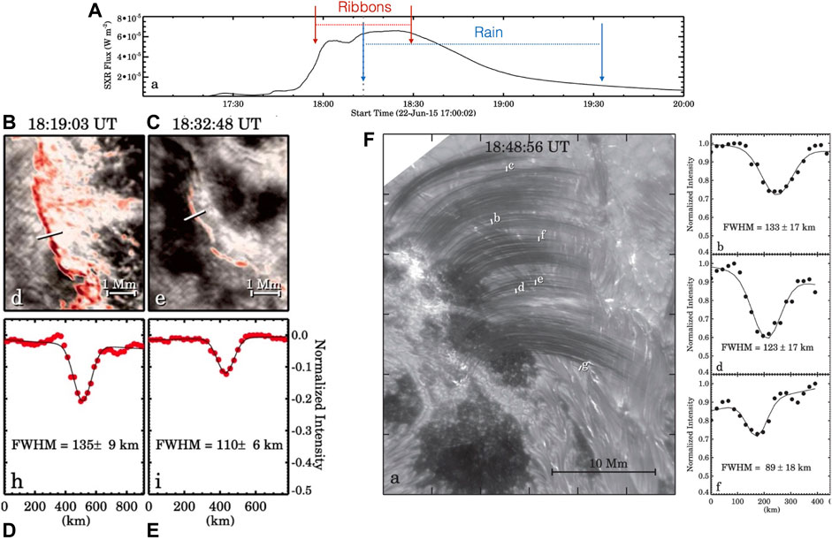
FIGURE 17. Fine structure produced by a solar flare observed in Hα with the NST, reported by Jing et al. (2016). (A) shows the GOES soft X-ray 1–8 Å  light curve, where the temporal location of the flare ribbons (in red) and the flare-driven rain (in blue) are indicated. (B–E) show the ribbon in Hα at 2 instances in time. The intensity along a cut across the ribbon (in white) is shown in the bottom panels, with the respective FWHM values from the fits. (F), a snapshot of the Hα FOV is shown during the gradual phase, where the rain can be seen in absorption. The intensities and the respective fits along several cuts across the strand-like rain structure are shown on the (F). Note that the FWHM values of the rain widths match the widths of the ribbons. Adapted from Figures 1, 2 and 3 of Jing et al. (2016).

An additional variability component of active regions is produced by the impact of the rain in the lower atmosphere. As most of the rain is observed to reach speeds of 150 km s⁻¹ or more at lower heights, it may either strongly decelerate prior to impact, case in which a shock is produced due to its supersonic speeds, or directly collide with the denser layers (see Figure 16). In both cases, a brightening event is expected at transition region and chromospheric levels. Evidence for the former has been reported by Straus et al. (2015), Schad et al. (2016), but the latter seems to be more frequent (Kleint et al., 2014; Antolin et al., 2015; Samanta et al., 2018; Chen et al., 2022). This can be explained by the fact that while individual rain clumps have kinetic energies in the nanoflare range, showers have energies in the microflare range. A UV and EUV imprint is therefore expected from rain impact. This is also observed from prominence fallback following eruptions (Reale et al., 2014), which is argued that could serve as template for stellar accretion. The long-lived supersonic and dense downflows produced by the hybrid prominence/coronal rain kind may be particularly relevant in this aspect, due to its larger integrated energy over time.

As mentioned in section 2.2.3, coronal rain has a multi-stranded structure and it is usually assumed that it is a good local and, as it falls, a global tracer of the coronal magnetic field. This is particularly questionable when observing in spectral lines from neutral atoms such as Hα, where field line tracing is not guaranteed. This is indeed expected because of the very strong ion-neutral coupling. Significant deviations on the order of the clump’s width would be achieved for ionisation fractions on the order of 10^–5 − 10^–4, but 100–1,000 times higher ionisation values are predicted based on photoionisation from the lower atmosphere alone (Heasley and Mihalas, 1976). This does not mean, however, that an apparently continuous strand-like structure at a given time reflects the local or global topology of the magnetic field. While the trajectory of each part of a rain clump will follow the magnetic field, the fact that clumps extend transversely over a significant width of a few Mm (a shower’s width), each subject to slightly different thermodynamic conditions and thus downward velocities, can lead to apparently misaligned clumps (Claes et al., 2020; Antolin et al., 2022).

In addition to TNE-TI cycles serving as a proxy for coronal heating mechanisms, the occurrence of this phenomena, and in particular coronal rain, can be used as a proxy to measure important in situ physical quantities. For example, coronal magnetic field measurements have been made using long-lived coronal rain events, such as in hybrid prominence/coronal rain complexes, which allow long integration times to build significant signal in Stokes parameters for spectro-polarimetric inversions. Schad et al. (2016, 2021) are able to find the variation of the magnetic flux with height, changing rapidly from 50 G at 40 Mm height, to values above 1000 G at 10 Mm height (Figure 18). The weak field approximation (Landi Degl’Innocenti and Landolfi, 2004; Centeno, 2018) provides a reliable estimation of the magnetic flux without the need of long integration times, provided that the Zeeman width of the line is much smaller than the Doppler width (i.e., for relatively small magnetic field strengths) and that the magnetic field is constant along the LOS (which is usually the case for off-limb observations). While the WFA provides the LOS component of the field, the total magnitude can be inferred from the rain’s trajectory, which in turn can be known from the ratio between the POS and Doppler (LOS) velocity component. Using this, Kriginsky et al. (2021) infer total field values of 500 G (with minima/maxima of 200/1,000 G) at heights of $\approx 10$Mm above the limb (probably, 15–20 Mm heights or so above the surface) in an active region (see Figure 18), consistent with the measurements of Schad et al. (2016). These coronal magnetic field measurements are striking since they are a factor of 10 larger than usually assumed coronal magnetic field values in the corona. More observations are needed to confirm whether this picture. As discussed below, this has strong consequences for coronal heating mechanisms, e.g. MHD waves.

FIGURE 18

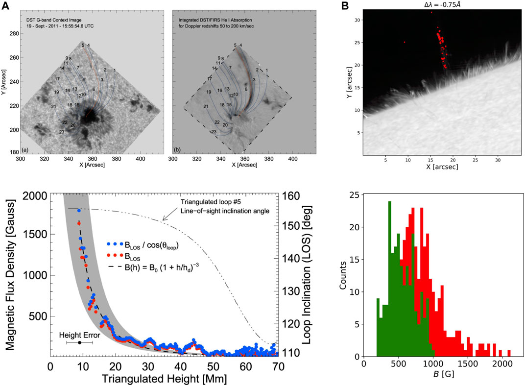
FIGURE 18. Magnetic field measurements from coronal rain observations. (A) the 2 panels on top show coronal rain (likely of the hybrid kind) detected in the He I 10 830 line with DST/FIRS, continuously falling along a coronal loop onto a sunspot umbra, reported by Schad et al. (2016) (Figures 3 and 8 of that paper © AAS. Reproduced with permission). Spectropolarimetry is performed to infer the coronal magnetic flux along the loop with respect to the triangulated height (LOS component in red, total component in blue inferred from the measured inclination of the loop through triangulation). (B) SST observations in the Ca II 8542 line (top panel shows the spectral position shifted −0.75 Å  from line centre) of quiescent coronal rain at the limb, reported by Kriginsky et al. (2021) (Figures 4 and 9 of that paper, reproduced with permission © ESO). Red points overlaid on the top panel denote locations where the WFA method was successfully applied to infer the LOS magnetic field. The total magnetic field distribution is shown in the bottom, calculated using the loop inclination derived from the POS to LOS velocity ratio. The green and red histograms denote, respectively, the measurements for which the Zeeman width is lower and higher than the Doppler width. Note that the WFA condition formally applies in the former case (green histogram). See the text and the respective papers for further details.

Another important physical quantity that can be estimated from coronal rain observations is the non-thermal line broadening, which provides a measure of turbulence in coronal loops. This quantity can be used to estimate the amplitudes from transverse MHD waves (Pant and Doorsselaere, 2020), and therefore their energy flux and potential role in coronal heating. As stated in section 2.2.3, non-thermal line broadening can vary significantly depending on the event, with loops showing average values between 5–10 km s⁻¹ only (Antolin et al., 2015; Kriginsky et al., 2021) while others show values of 8–16 km s⁻¹ (with a tail up to 22 km s⁻¹), that is, on the same order or larger than the thermal component Froment et al. (2020), see Figure 10. It is interesting to note that the 15–20 km s⁻¹ range is common in active region loops with temperatures between 1 MK and 5 MK (Chae et al., 1998; Hara and Ichimoto, 1999; Brooks and Warren, 2016; Testa et al., 2016), and also with that obtained from models based on either MHD waves (Shi et al., 2021) or field-line braiding (Pontin et al., 2020), which suggests that the same level of turbulence can be found in loops with or without TNE. In other words, and rather counter-intuitively, the TNE process (which is known to induce strong flows along the loop), does not necessarily lead to higher levels of turbulence. This constancy of the non-thermal velocity may suggest that turbulence-based heating mechanisms (such as transverse MHD waves or Alfvén waves) that are usually expected to act uniformly in the coronal portions of loops (Matsumoto, 2018), do not play a direct role in coronal heating in active regions. Otherwise, the observed turbulence-based mechanism would actively inhibit the onset of TNE, as also shown by Antolin and Shibata (2010). A detailed study of the non-thermal velocity during TNE cycles is needed in order to confirm this.

Using the non-thermal velocity measurements from coronal rain and an average magnetic field value of 500 G from Kriginsky et al. (2021) (at the same height as the non-thermal broadening measurements) we can also calculate an upper limit for the Alfvén wave energy flux (assuming that the amplitude of the wave is equal to the non-thermal broadening) of $\frac{1}{2}\rho {(\delta v)}^2{v}_A\approx 10^7$erg cm⁻² s⁻¹, taking an average number density for the loop of 5 × 10⁹ cm⁻³. If kink waves are observed instead (Antolin and Verwichte, 2011; Kohutova and Verwichte, 2016), the wave energy flux is on the order of 5 × 10⁵–10⁶ erg cm⁻² s⁻¹ for a filling factor of 5% (Van Doorsselaere et al., 2014). These are significant values for wave energies, of the same order as that required for active region coronal heating. The debate of whether Alfvénic waves are important or not for coronal heating therefore remains.

Besides the transverse MHD wave tracing capabilities of coronal rain mentioned in section 2.2.3, the rain can also provide insight on the reconnection dynamics, as recently shown by Antolin et al. (2021). Indeed, fast ($\approx 100$ km s⁻¹), short-lived (10–20 s) and tiny (500 km in widths, 1,500 km in lengths) jet-like phenomena, termed nanojets, with energies in the 10²⁴ erg nanoflare range, were detected with IRIS in a hybrid prominence/coronal rain structure (Figure 19). The nanojets are interpreted as component (small-angle) reconnection within a loop, with magnetic tension advecting the heated plasma sideways (Pagano et al., 2021). The nanojets are further characterised by being perpendicular to the coronal loop structure, unidirectional (in contrast with the expected bi-directional outflows expected from reconnection), with some having plasmoid-like structures ejected along their lengths. Antolin et al. (2022) report myriad nanojets (150 events in 13 min) accompanying the formation of a hot (5 MK) coronal loop, with an evolution similar to that of an MHD avalanche. The nanojets therefore correspond to a direct observational signature of the reconnection-driven nanoflare in the corona, as predicted by Parker (1988). Besides the local features such as the nanojets, the coronal rain in the loop further allows to visually trace the global coronal loop structure, and in particular the presence of braiding, which is observed to decrease as the heating unfolds. In this picture, the rain acts as a tracer but it is also possible that it acts as a catalyst of the reconnection process by increasing the resistivity through its partially ionised nature.

FIGURE 19

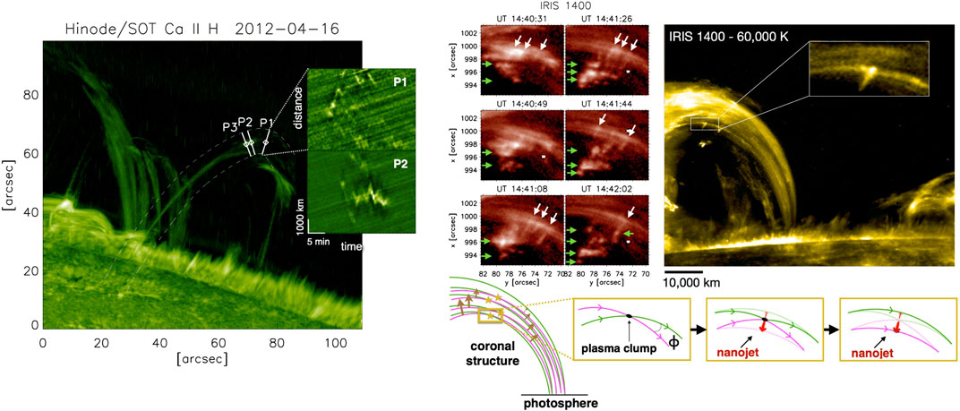
FIGURE 19. Coronal rain as a tracer of coronal heating mechanisms. Left: a Hinode/SOT observation in the Ca II H line reveals several loops with coronal rain, reported by Verwichte et al. (2017) (Figures 4 and 5 of that paper, reproduced with permission © ESO). The 2-panel inset shows the time-distance diagram across transverse cuts P1 and P2 near the apex of a loop. Transverse MHD oscillations can be clearly seen. Right: Nanojets observed in a hybrid prominence/coronal rain complex with IRIS/SJI 1400, reported by Antolin et al. (2022) (adapted from Figures 1, 2 and 6 of that paper). The left 6-panels show a time sequence in which a nanojet cluster can be seen (white arrows), some ejecting plasmoids (green arrows). The bottom panel shows a sketch of the interpretation. Component magnetic reconnection leads to localised heating and transverse advection of reconnected field lines driven by magnetic tension, resulting in the nanojet feature. See the respective papers for further details.

3.3 What Properties of Solar Active Regions Thermal Non-Equilibrium-Thermal Instability Can and Cannot Explain

3.3.1 Key Properties of Coronal Loops

On top of reproducing the recently discovered long-period intensity pulsations, TNE is able to reproduce key observables of coronal loops. Lionello et al. (2013), Winebarger et al. (2018) showed that TNE simulations are compatible with eight key loop observables (Klimchuk, 2006):

• the observed over-density of active region loops,

• the density stratification that is lower than for hydrostatic equilibrium (Aschwanden et al., 2001),

• the relatively flat temperature profile in the corona,

• the apparent constant cross-section of coronal loops with height,

• the smooth intensity variation along the loops (usually no strong and localized brightenings),

• the long life time of loops (usually from 15 to 90 min, relative to their cooling time)

• the EUV cooling delay between passbands (see section 2.2.1),

• the broad DEM, as observed in active regions (Winebarger et al., 2011).

To these, we may of course add that TNE is also able to reproduce the observed long-period intensity pulsations and coronal rain.

3.3.2 The Diffuse Emission

Coronal loops are the most distinguishable structures of the corona of solar active regions. They often serve as a proxy for studying flux tubes in the solar atmosphere and were, as a consequence, extensively studied (Reale, 2014). They are bright structures contrasting with their environment even though there are actually only 10%–30% brighter than the surrounding material (e.g., Del Zanna and Mason, 2003). The bulk of the active region volume is in fact composed by the so-called “diffuse emission”. This emission is produced by the plasma in the background and foreground of loops and around them, encompassing the active regions. The diffuse emission, albeit predominant, has been underinvestigated compared to coronal loops (Klimchuk, 2006).

The knowledge on these regions is therefore rather limited. Many works however have considered nanoflare heating in order to explain the diffuse emission (e.g., Viall and Klimchuk, 2012, 2013; Cargill, 2014; Cargill et al., 2015). Klimchuk (2015) in particular, proposed a unified picture in order to explain both the diffuse emission and the coronal loop emission. The first one would come from weak, high-frequency and scattered nanoflare events, while the second one would come from strong, low-frequency and localised nanoflare events. The nanoflare frequency has been investigated using the slope of the DEM (see section 2.2.1) (Del Zanna and Mason, 2003; Del Zanna, 2013; Subramanian et al., 2014; Del Zanna et al., 2015). Steep slopes, corresponding to more isothermal DEMs may indicate high-frequency nanoflares, while weaker slopes may indicate low-frequency nanoflares. In the later the plasma has more time to cool down between the heating events which result in more cool material along the line-of-sight. One should nonetheless bear in mind that this slope is poorly constrained by observations (Guennou et al., 2013).

Viall and Klimchuk (2013) showed that a steady and uniformly distributed heating along the coronal loops length would produce quasi-steady light curves and thus would not show a pattern of cooling as coronal loops do. However, in observations such cooling pattern is widespread in active regions (Viall and Klimchuk, 2012) and therefore Viall and Klimchuk (2013) conclude that steady heating can not be at play to produce the diffuse emission. However, quasi-steady heating can also reproduce the EUV cooling pattern, if the heating is stratified. This is what is observed for loops showing long-period intensity pulsations and TNE signatures (see section 2.2.1).

It is unclear if TNE could also participate in the formation of the diffuse emission. The statistics presented in Auchère et al. (2014) with EIT/SoHo and Froment (2016) with AIA/SDO statistics pulsations show that about 50% of long-period intensity pulsations events are found in active regions. Depending on the EUV channel used, at most 50% of these active region events are visually associated with distinguishable loops. Up to now only the loops events have been investigated in details. It is thus unclear whether the other active region events are also a manifestation of TNE. These events should be investigated to see whether at least some of them are linked to the diffuse emission and whether TNE can be at play in these regions. The left panel of Figure 20 presents an example of such active region event. Taking into account the fact that TNE seems to play an important role for many coronal loops systems, it is natural to think that footpoint heating may play an important role for active regions as a whole. As developed in Froment et al. (2018), different loop geometries can lead to different plasma response (TNE or no TNE) when the heating is similar. Adding a distribution of heating frequencies to the distributions of loop geometries and other heating parameters could naturally explain different plasma response within an active region. Extensive observational and numerical work would be required to investigate this possibility.

FIGURE 20

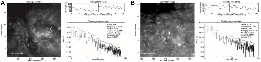
FIGURE 20. Detection of pulsations outside of loops structures. (A) Pulsations detected in an active region but that does not appear to be linked to a visible loop structure. (B) Pulsations detected in the quiet Sun. In each panel the SoHO/EIT 195 Å field-of-view is presented in heliographic coordinates. The top light curves are averaged over the white contour in the images. The Fourier spectra of these light curves are presented below. Both Figures are adapted from Auchère et al. (2014) (Figures 2, 3, reproduced with permission © ESO). See the original paper for more details.

3.3.3 Short Timescale Dynamics

TNE is a global process, able to shape the dynamics of a loop bundle at large scales, leading to long timescales of several days (periodicities of hours), across loop bundles and along large loops. As shown in Froment et al. (2017), TNE simulations reproduce very well the envelope of the light curves, meaning the low-frequency fluctuations only. However, short timescale dynamics (lower than the radiative cooling time) are a common feature of coronal loop light curves. These may correspond to localised heating events, and thus to signatures of the coronal heating mechanisms. It is unclear whether adding a distribution of heating frequencies in TNE simulations would be enough to reproduce the observed short timescale variations. On the other hand, TI is a local phenomenon occurring on much faster timescales, and we have seen that TI onset also leads to signatures in the EUV which can have a global character (e.g., strand-like morphology). It is therefore possible that forward modelling of multi-dimensional simulations of TNE-TI can also reproduce the short timescale dynamics to some extent. One should also bear in mind that these short timescale fluctuations can also come from other structures in the background or foreground of pulsating loops and that 1D hydrodynamical simulations of a single loop, such as in Froment et al. (2017), cannot reproduce such dynamics.

3.3.4 Active Region Core Loops

Although TNE can be produced in very short loops on the scales of those seen in active region cores or shorter (eg., Mendoza-Briceño et al., 2005), TNE signatures (such as coronal rain or EUV pulsations) are not usually observed in those loops. A major difference with loops undergoing TNE are the hot temperatures usually detected all along their lengths ($\approx 4$ MK or higher, e.g., Del Zanna and Mason, 2014). Hydrodynamic models suggest a steady (high-frequency) heating (Winebarger et al., 2011) with loops close to equilibrium, satisfying the RTV scaling law (Rosner et al., 1978; Martens, 2010). This is supported partly by observations displaying very little intensity variability in the moss region (Warren et al., 2020), while other observations of active region cores provide evidence of strong variability, linked to either coronal nanoflares or magnetic flux cancellation events (Testa et al., 2014; Chitta et al., 2018; Tiwari et al., 2019).

Assuming that high-frequency heating is generally the case for active region core loops, TNE theory indicates that the heating must not be too stratified for TNE to be suppressed. Winebarger et al. (2008) conduct modelling to match the observed X-ray intensity from active region core loops, obtaining a heating rate that scales as B^0.29L^−0.95. Such scaling law suggests very mild footpoint heating, in agreement with theory to avoid TNE.

3.4 TNE in Quiet Sun Regions and Relationship With Open-Field Line Topologies

As previously developed in Section 2.2.5, coronal rain is also observed near X-point structures. These hybrid prominence/coronal rain complexes have been observed in both active region and quiet Sun and some of them can be linked to open-field regions. The magnetic dips that may form in such magnetic topologies act as mass reservoirs and thus may feed the generation of long-lived coronal rain showers that are usually seen above active regions (Chen et al., 2022). Reconnection between open and closed field lines, also known as interchange reconnection (Fisk and Schwadron, 2001; Crooker et al., 2002) may also take place in these structures as hypothesized by Mason et al. (2019), Li et al. (2020). Their exact relationship with TNE and thus a quasi-steady and stratified heating, remains to be investigated. In particular, the periodicity of their TNE cycles, if any. Since hybrid prominence/coronal rain structures constitute an important mass and energy reservoir, they may play an important role in the solar wind formation.

On the other hand, Auchère et al. (2014), Froment (2016) found that 50% of their long-period intensity pulsation events occur in the quiet Sun. The right panel of Figure 20 shows an example of such event. They seem to have in general longer periods than active region events. If they are also a manifestation of TNE cycles in the corona, as we have seen in Section 2.1.1, longer periods may imply longer structures. The pulsations found in the quiet Sun might thus be linked to very long structures, possibly connected to active regions. If this is the case, we hypothesise that coronal rain should be observed at the other, active region end of the observed structures. The observed pulsations might actually correspond to only a subset of such large structures.

Recently, Schlenker et al. (2021) investigated the possible effect of TNE on helmet streamers using 2.5 MHD simulations. In their simulations, they produce coronal rain falling back toward the footpoints of the very large helmet streamer loops and continuous plasmoid ejection toward the solar wind. They argue that TNE is likely to be present in coronal loops at the boundaries of coronal holes and that it might explain the persistent blue-shifts observed at the boundaries of active regions (Tu et al., 2005; Sakao et al., 2007; Tian et al., 2021). Helmet streamers, high up in the corona can also serve as mass and energy reservoirs for the solar wind. Investigating TNE in helmet streamers in the observations would thus allow to both investigate coronal heating processes and solar wind drivers.

4 Current Research Gap and Future Challenges

Thermal non-equilibrium and thermal instability in the solar corona are two currently highly active fields of research, spearheaded by the recent discovery of the widespread long period intensity pulsations, the recent realisation of the importance and ubiquity of coronal rain, and the strong link between both phenomena. Great advances have been achieved on the observational side, with the advent of high resolution instrumentation that cover for the first time the wide temperature and multi-scale gap of the physical processes involved in TNE-TI in the solar atmosphere. Similarly, on the numerical side major advances have been achieved, with multi-dimensional simulations and spectroscopic codes incorporating in effective ways the required very high resolution and non-adiabatic effects, thus allowing to probe into the physics of TNE-TI. The emerging picture is that of a mechanism extremely rich in physical processes, strongly linked to some of the most pressing open questions in astrophysics. Furthermore, a strong connection with other fields at much larger scales in the Universe makes this field of research highly cross-disciplinary.

The following are open questions/future challenges that need to be addressed with the advent of next generation instrumentation, larger computational power and big data analysis.

4.1 Observational Side

• What is the fraction of the coronal volume that is controlled by TNE and that subject to thermal instability? How pervasive is coronal rain? How does these volume fractions vary across the solar cycle? Recent observations indicate that the TNE volume within an active region could be on the same order as the coronal volume (Şahin and Antolin, 2022, manuscript in preparation), but a large variation from region to region may be expected. Current Fourier-based detection methods for EUV pulsations only provide a tip-of-the-iceberg picture, excluding all non-highly periodic events. Auchère et al. (2014) estimated that at least about 50% of the active regions undergo long-period intensity pulsations. These are the very periodic cases, detected with a conservative method. These are the unusually stable cases. We can thus consider this number as a lower limit. Moreover, as seen by numerical simulation studies, quasi-constant and stratified heating does not always produce TNE (see Section 2.1.1.)

• How common are hybrid prominence/coronal rain complexes? These structures can provide a sustained mass and energy reservoir for the neighboring corona. Does interchange reconnection play a major role, and if so, should we expect an important contribution on the solar wind?

• How is flare-driven rain generated and how common is it? Should we expect it in all flares, and is the rain quantity highly correlated to the energy release? Its occurrence suggests an important contribution from either a secondary mechanism besides electron beams or from multi-dimensional effects.

• Can we infer the heating conditions from the observed properties of long-period intensity pulsations and coronal rain? We have seen the existence of stringent conditions for heating stratification, frequency of the heating events and geometric and heating asymmetries for TNE-TI occurrence. Similarly, the thermodynamics and kinematics of the rain can be used to reveal turbulence, heating agents and force balance within loops.

• What is the true morphology of the rain clumps? Increasingly higher spatial resolution reveals a tip-of-the-iceberg distribution, with increasingly higher clump numbers. Simulations indicate distinct morphologies, such as splattering, shattering and so forth (Waters and Proga, 2019; Gronke and Oh, 2020), which are strongly linked to the character of thermal instability and interaction between modes. In turn, TI depends on non-adiabatic effects, such as the radiative losses, turbulence, parallel and perpendicular thermal conduction coefficients, making the problem complex.

• What is behind the shower morphology? Do showers undeniably require the existence of a syncing mechanism between critically stable coronal loops? Observations and simulations of showers indicate this possibility (see section 2.2.3, Antolin and Rouppe van der Voort, 2012; Fang et al., 2015).

4.2 Numerical Side

• What are the spatio-temporal properties of the heating at the footpoints of coronal structures? Most the numerical studies we have mentioned in the present review are based on ad hoc heating functions. These are very useful in order to test the response of the plasma and to determine the observables to look for. However, the link with the boundary conditions imposed by the solar magnetoconvection is missing. The constant emergence and cancellation of the magnetic flux imply that the boundary heating conditions will vary. This is challenging to reconcile with the week-long and quasi-steady long-period intensity pulsations.

• What are the properties of TNE-TI in self-consistent and realistic 3D MHD simulations? Only recently, coronal rain has been produced in 3D radiative MHD codes that self-consistently treat the heating. However, these codes still lack the required resolution at transition region and coronal levels to properly model the chromospheric evaporation process and the small-scale morphology of the rain clumps. Furthermore, the investigation of long period intensity pulsations requires many hours of computing time, which makes the task even more challenging.

• Does coronal rain exclusively correspond to unstable thermal modes? In the complex solar atmosphere, it has been shown that unstable modes can have mixed properties, and that all MHD modes may become unstable (Claes and Keppens, 2021; Zavershinskii et al., 2021). This is linked to the observed morphology of clumps, as discussed above.

• What is the role of dynamic instabilities and turbulence in the generation of coronal rain? Numerical work shows that RT-type instabilities should occur at loop apexes for weak magnetic fields (Moschou et al., 2015; Xia et al., 2017). These, however, are expected to be suppressed in active region loops for which the magnetic field strength is high. Also, the typical plume-like structure produced by such instabilities is not observed. On the other hand, numerical work in the ISM shows that the turbulence generated by dynamic instabilities is key to the formation of condensations (Gronke and Oh, 2018; Fielding et al., 2020), thanks to the very efficient mixing between cool and hot plasma (thus enhancing the radiative losses), as discussed in the next section.

4.3 Stellar and Astrophysical Implications/Similarities

Recent advances from solar to extra-galactic physics have shown several similarities between these cycles, driven by scale-free fundamental physical processes whose understanding constitute some of the greatest challenges in astrophysics.

We have seen in the previous sections that a measured cooling response in the form of coronal rain can exist due to heating, and a good correlation should exist between the amount of coronal rain, as well as TNE volume exhibiting EUV pulsations, and the amount of energy release. It is natural to wonder whether this tendency can be extrapolated to stars in general, for which much larger scales and energies can be involved. Magnetically active stars exhibit recurrent optical and UV red-shifts (Reale et al., 2013; Fuhrmeister et al., 2018), and coronal rain appears as a prime candidate to explain such features (Ayres and France, 2010; Ayres, 2015). Along this line of thought, given that the TNE volume appears to be significant in the solar atmosphere, it is worth considering whether TNE cycles in other stars could be detectable.

Besides the solar corona, systems with heating and cooling processes leading to self-regulating mass and energy cycles exist at much larger scales in the Universe. At the large scales of galaxy formation, observations indicate a strong correlation between the hot 10⁷–10⁸ K ICM medium, the presence of multiphase gas in the form of filamentary molecular clouds, and star formation in the cool cluster cores (White and Rees, 1978; Cavagnolo et al., 2008; Dunn and Fabian, 2008; Prasad et al., 2015). A promising hypothesis behind this multi-scale relation in the ICM (or CGM) evolution relies on a feedback mechanism, also known as the “the precipitation limit” (Voit et al., 2015, 2019), in which thermal instability plays a central role. While the heating mechanisms of the ICM are still under debate, it is generally accepted that the cooling via thermal instability and the subsequent dense multiphase “galactic rain,” downward onto the central supermassive black hole energises the outflows driven by accretion. These outflows, in turn, control the density and temperature of the ICM (McNamara and Nulsen, 2007; Rafferty et al., 2008), as well as the formation and destruction of multiphase gas through dynamic instabilities and mixing (Gronke and Oh, 2018; Tan et al., 2021), thereby regulating the precipitation.

In section 2.2.3 we have seen that the morphology of multiphase plasma such as coronal rain is strongly linked to the details of the radiative cooling function, the thermal and dynamic instabilities and the force balance within coronal loops. Similarly, thermal and dynamic instabilities have long been invoked to explain the observed filamentary, multiphase structure in the ISM and ICM (Sharma et al., 2010; Sharma, 2013; Waters and Proga, 2019; Kanjilal et al., 2021). 3D MHD simulations have shown that dynamic instabilities (such as KHI) and the generated turbulence play an essential role in the formation and destruction of multiphase plasma in the ICM (Gronke and Oh, 2018; Fielding et al., 2020). The details of the thermal instability-driven cooling rate and the structure of the eigenmodes, whose theory is greatly extended in the ISM/ICM fields (e.g., Waters and Proga, 2019; Kanjilal et al., 2021), directly influence the quantity and morphology of the multiphase plasma, which are still under debate in the ISM/ICM due to the lack of direct observational constraints (Gronke and Oh, 2020). On the other hand, as we have seen, coronal rain is similarly clumpy and filamentary, and the solar corona, as the ISM and ICM, can be magnetically dominated and turbulent (Fabian et al., 2008; Zhuravleva et al., 2014). Coronal rain observations may therefore serve as a template for ISM/ICM multiphase plasma morphologies and dynamics. Furthermore, the routes to unstable evolution of the full spectrum of linear MHD eigenmodes can now be considered in non-trivial magnetic configurations taking into account non-adiabatic (Claes and Keppens, 2021) and thermal misbalance effects (Kolotkov et al., 2021) with recently developed codes inspired by solar condensations (Claes et al., 2020).

The phenomenon of accretion of cold material is observed in most cosmic objects in the Universe. Interestingly, the dynamics of multiphase plasma within molecular loops in the Galactic centre presents similar dynamics as coronal rain (Fukui et al., 2006; Torii et al., 2010). Being so close, coronal rain or prominence eruption fallback can serve as a template for stellar and ICM accretion (Reale et al., 2013). In the solar context, as seen in section 2.2.3, the final speeds are observed to be much lower than free-fall, which appear linked to gas pressure restructuring downstream of the rain. The signature of this deceleration mechanism is the existence of a peculiar mass-velocity relation, predicted by numerical simulations but whose physics are still unclear (Oliver et al., 2014; Martínez-Gómez et al., 2020). A natural question is therefore whether such process is at work in the ISM/ICM. Such dynamics are important since they regulate the ratio of the cooling time to the free fall time τ_rad/τ_ff (cf. section 2.2.4), a key parameter in the ICM that dictates the amount of material that is subject to condensation (Sharma, 2013; Choudhury and Sharma, 2016; Choudhury et al., 2019).

The formation of the galactic loops with multiphase material poses a formidable puzzle, and possible explanations have been sought in solar prominence models (Peng and Matsumoto, 2017). On the other hand, the TNE-TI model of evaporation and condensation leading to coronal rain is a more natural scenario that awaits investigation. Recent realistic, global-scale 3D MHD simulations of coronal rain and prominences (Xia et al., 2014; Moschou et al., 2015; Kaneko and Yokoyama, 2017; Xia et al., 2017) can therefore shed light upon the possible origin of molecular Galactic loops.

Yet another topic in which interesting applications can be found concerns a star’s rotational evolution, which crucially depends on its mass loss rate via its wind. A major observational gap is presented since the hot and tenuous stellar wind of cool stars is extremely difficult to detect. Such stars can support “slingshot prominences” (Robinson and Collier Cameron, 1986; Steeghs et al., 1996), which are far easier to observe and have been shown to be potentially significant contributors to the stellar wind, thereby acting as “wind gauges” (Jardine and Collier Cameron, 2019). Yet, this proxy crucially depends on the formation and removal of the condensations from the star’s co-rotation radius. The TNE-TI model may therefore be applicable and shed light into the wind gauge mechanism.

Author Contributions

PA and CF drafted the plan of the manuscript. PA wrote most of the manuscript. CF mainly wrote the sections concerning TNE theory and observations (Sections 2.1.1 and 2.2.1 and Sections 3.3 and 3.4). PA and CF edited together the final draft.

Funding

PA acknowledges STFC support from Ernest Rutherford Fellowship grant number ST/R004285/2. CF acknowledges funding from the CNES. Both authors acknowledge funding from the International Space Science Institute, Bern, Switzerland.

Conflict of Interest

The authors declare that the research was conducted in the absence of any commercial or financial relationships that could be construed as a potential conflict of interest.

The handling Editor declared a past co-authorship with one of the authors PA.

Publisher’s Note

All claims expressed in this article are solely those of the authors and do not necessarily represent those of their affiliated organizations, or those of the publisher, the editors and the reviewers. Any product that may be evaluated in this article, or claim that may be made by its manufacturer, is not guaranteed or endorsed by the publisher.

Acknowledgments

We would like to thank the two referees for their valuable contribution during the reviewing process of this manuscript. CF and PA acknowledge support from the International Space Science Institute, Bern, Switzerland to the International Team on “Observed Multi-Scale Variability of Coronal Loops as a Probe of Coronal Heating”. CF and PA acknowledge the fruitful discussions and work with the members of both teams. The SST is operated on the island of La Palma by the Institute for Solar Physics of Stockholm University in the Spanish Observatorio del Roque de los Muchachos of the Instituto de Astrofísica de Canarias. Hinode is a Japanese mission developed and launched by ISAS/JAXA, with NAOJ as domestic partner and NASA and STFC (UK) as international partners. It is operated by these agencies in co-operation with ESA and NSC (Norway). IRIS is a NASA small explorer mission developed and operated by LMSAL with mission operations executed at NASA Ames Research Center and major contributions to downlink communications funded by ESA and the Norwegian Space Centre. SDO is part of NASA’s Living With a Star Program.

Footnotes

¹Defined here as the MHD waves for which transverse displacements dominate over longitudinal displacements, i.e., having either magnetic tension or magnetic pressure as a major restoring force.

²It would be incorrect to assume that this kind corresponds to a prominence whose magnetic support locally breaks, since this would incorrectly imply the existence of a prominence in the first place. On the other hand it is more likely that such a hybrid structure gives birth to a prominence in the long run

³It is important to note that limits to the efficiency of chromospheric evaporation are expected, based on where the energy from the flare is deposited in the lower atmosphere, which in turn depends on the details of the energy release (Reep et al., 2015)

References

Adrover-González, A., Terradas, J., Oliver, R., and Carbonell, M. (2021). Gravitational Instability of Solar Prominence Threads. A&A 649, A142. doi:10.1051/0004-6361/202039677

CrossRef Full Text | Google Scholar

Ahn, K., Chae, J., Cho, K.-S., Song, D., Yang, H., and Goode, P. R. (2014). Active Region Coronal Rain Event Observed by the Fast Imaging Solar Spectrograph on the NST. Sol. Phys. 289, 4117–4136. doi:10.1007/s11207-014-0559-x

CrossRef Full Text | Google Scholar

Anfinogentov, S. A., Nakariakov, V. M., and Nisticò, G. (2015). Decayless Low-Amplitude Kink Oscillations: a Common Phenomenon in the Solar corona? A&A 583, A136. doi:10.1051/0004-6361/201526195

CrossRef Full Text | Google Scholar

Antiochos, S. K., and Klimchuk, J. A. (1991). A Model for the Formation of Solar Prominences. Astrophysical J. 378, 372–377. doi:10.1086/170437

CrossRef Full Text | Google Scholar

Antiochos, S. K., MacNeice, P. J., Spicer, D. S., and Klimchuk, J. A. (1999). The Dynamic Formation of Prominence Condensations. Astrophysical J. 512, 985. doi:10.1086/306804

CrossRef Full Text | Google Scholar

Antiochos, S. K. (1980). A Model of Active Prominences. ApJ 236, 270–279. doi:10.1086/157743

CrossRef Full Text | Google Scholar

Antolin, P., and Rouppe van der Voort, L. (2012). Observing the Fine Structure of Loops through High-Resolution Spectroscopic Observations of Coronal Rain with the CRISP Instrument at the Swedish Solar Telescope. Astrophysical J. 745, 152. doi:10.1088/0004-637X/745/2/152

CrossRef Full Text | Google Scholar

Antolin, P., and Shibata, K. (2010). The Role of Torsional Alfvén Waves in Coronal Heating. ApJ 712, 494–510. doi:10.1088/0004-637X/712/1/494

CrossRef Full Text | Google Scholar

Antolin, P., and Verwichte, E. (2011). Transverse Oscillations of Loops with Coronal Rain Observed by Hinode/Solar Optical Telescope. ApJ 736, 121. doi:10.1088/0004-637X/736/2/121

CrossRef Full Text | Google Scholar

Antolin, P., Shibata, K., Kudoh, T., Shiota, D., and Brooks, D. (2008). Predicting Observational Signatures of Coronal Heating by Alfvén Waves and Nanoflares. ApJ 688, 669–682. doi:10.1086/591998

CrossRef Full Text | Google Scholar

Antolin, P., Shibata, K., and Vissers, G. (2010). Coronal Rain as a Marker for Coronal Heating Mechanisms. Astrophysical J. 716, 154–166. doi:10.1088/0004-637X/716/1/154

CrossRef Full Text | Google Scholar

Antolin, P., Vissers, G., and Rouppe van der Voort, L. (2012). On-Disk Coronal Rain. Solar Phys. 280, 457–474. doi:10.1007/s11207-012-9979-7

CrossRef Full Text | Google Scholar

Antolin, P., Vissers, G., Pereira, T. M. D., Voort, L. R. v. d., and Scullion, E. (2015). The Multithermal and Multi-Stranded Nature of Coronal Rain. Astrophysical J. 806, 81. doi:10.1088/0004-637X/806/1/81

CrossRef Full Text | Google Scholar

Antolin, P., Martínez-Sykora, J., and Şahin, S. (2022). Thermal Instability Induced Fundamental Magnetic Field Strands in the Solar corona. Astrophys. J. Lett. 926 (2), L29. doi:10.3847/2041-8213/ac51dd

CrossRef Full Text | Google Scholar

Antolin, P., Pagano, P., Testa, P., Petralia, A., and Reale, F. (2021). Reconnection Nanojets in the Solar corona. Nat. Astron. 5, 54–62. doi:10.1038/s41550-020-1199-8

CrossRef Full Text | Google Scholar

Antolin, P. (2020). Thermal Instability and Non-equilibrium in Solar Coronal Loops: from Coronal Rain to Long-Period Intensity Pulsations. Plasma Phys. Controlled Fusion 62, 014016. doi:10.1088/1361-6587/ab5406

CrossRef Full Text | Google Scholar

Aschwanden, M. J., Schrijver, C. J., and Alexander, D. (2001). Modeling of Coronal EUV Loops Observed with TRACE. I. Hydrostatic Solutions with Nonuniform Heating. ApJ 550, 1036–1050. doi:10.1086/319796

CrossRef Full Text | Google Scholar

Auchère, F., Bocchialini, K., Solomon, J., and Tison, E. (2014). Long-period Intensity Pulsations in the Solar corona during Activity Cycle 23. Astron. Astrophysics 563, A8. doi:10.1051/0004-6361/201322572

CrossRef Full Text | Google Scholar

Auchère, F., Froment, C., Bocchialini, K., Buchlin, E., and Solomon, J. (2016a). On the Fourier and Wavelet Analysis of Coronal Time Series. Astrophysical J. 825, 110. doi:10.3847/0004-637X/825/2/110

CrossRef Full Text | Google Scholar

Auchère, F., Froment, C., Bocchialini, K., Buchlin, E., and Solomon, J. (2016b). Thermal Non-equilibrium Revealed by Periodic Pulses of Random Amplitudes in Solar Coronal Loops. Astrophysical J. 827, 152. doi:10.3847/0004-637X/827/2/152

CrossRef Full Text | Google Scholar

Auchère, F., Froment, C., Soubrié, E., Antolin, P., Oliver, R., and Pelouze, G. (2018). The Coronal Monsoon: Thermal Nonequilibrium Revealed by Periodic Coronal Rain. Astrophysical J. 853, 176. doi:10.3847/1538-4357/aaa5a3

CrossRef Full Text | Google Scholar

Ayres, T., and France, K. (2010). Warm Coronal Rain on Young Solar Analog EK Draconis? ApJ 723, L38–L43. doi:10.1088/2041-8205/723/1/L38

CrossRef Full Text | Google Scholar

Ayres, T. R. (2015). The Flare-Ona of Ek Draconis. Astronomical J. 150, 7. doi:10.1088/0004-6256/150/1/7

CrossRef Full Text | Google Scholar

Balbus, S. A. (1986). Local Dynamic Thermal Instability. ApJ 303, L79. doi:10.1086/184657

CrossRef Full Text | Google Scholar

Ballester, J. L., Carbonell, M., Soler, R., and Terradas, J. (2018). The Temporal Behaviour of Mhd Waves in a Partially Ionized Prominence-like Plasma: Effect of Heating and Cooling. A&A 609, A6. doi:10.1051/0004-6361/201731567

CrossRef Full Text | Google Scholar

Beckers, J. M. (1964). A Study of the Fine Structures in the Solar Chromosphere. Ph.D. thesis. USA: Sacramento Peak Observatory, Air Force Cambridge Research Laboratories, Mass.

Google Scholar

Beckers, J. M. (1972). Solar Spicules. ARA&A 10, 73. doi:10.1146/annurev.aa.10.090172.000445

CrossRef Full Text | Google Scholar

Begelman, M. C., and McKee, C. F. (1990). Global Effects of Thermal Conduction on Two-phase Media. ApJ 358, 375. doi:10.1086/168994

CrossRef Full Text | Google Scholar

Bradshaw, S. J., and Cargill, P. J. (2005). The Cooling of Coronal Plasmas. II. Properties of the Radiative Phase. A&A 437, 311–317. doi:10.1051/0004-6361:20042405

CrossRef Full Text | Google Scholar

Bradshaw, S. J., and Cargill, P. J. (2013). The Influence of Numerical Resolution on Coronal Density in Hydrodynamic Models of Impulsive Heating. ApJ 770, 12. doi:10.1088/0004-637X/770/1/12

CrossRef Full Text | Google Scholar

Brooks, D. H., and Warren, H. P. (2016). Measurements of Non-Thermal Line Widths in Solar Active Regions. Astrophysical J. 820, 63. doi:10.3847/0004-637x/820/1/63

CrossRef Full Text | Google Scholar

Brynildsen, N., Maltby, P., Kjeldseth-Moe, O., and Wilhelm, K. (2001). Dual Flows and Oscillations in the Sunspot Transition Region. ApJ 552, L77–L80. doi:10.1086/320263

CrossRef Full Text | Google Scholar

Cargill, P. J., Warren, H. P., and Bradshaw, S. J. (2015). Modelling Nanoflares in Active Regions and Implications for Coronal Heating Mechanisms. Philosophical Trans. R. Soc. Lond. Ser. A 373, 20140260. doi:10.1098/rsta.2014.0260

PubMed Abstract | CrossRef Full Text | Google Scholar

Cargill, P. J. (2014). Active Region Emission Measure Distributions and Implications for Nanoflare Heating. Astrophysical J. 784, 49. doi:10.1088/0004-637X/784/1/49

CrossRef Full Text | Google Scholar

Cavagnolo, K. W., Donahue, M., Voit, G. M., and Sun, M. (2008). An Entropy Threshold for Strong Hα and Radio Emission in the Cores of Galaxy Clusters. ApJ 683, L107. doi:10.1086/591665

CrossRef Full Text | Google Scholar

Centeno, R. (2018). On the Weak Field Approximation for Ca 8542 Å 866, 89. doi:10.3847/1538-4357/aae087

CrossRef Full Text | Google Scholar

Chae, J., Schühle, U., and Lemaire, P. (1998). SUMER Measurements of Nonthermal Motions: Constraints on Coronal Heating Mechanisms. ApJ 505, 957–973. doi:10.1086/306179

CrossRef Full Text | Google Scholar

Chen, F., Rempel, M., and Fan, Y. (2021). A Comprehensive Radiative Magnetohydrodynamics Simulation of Active Region Scale Flux Emergence from the Convection Zone to the Corona. arXiv e-prints , arXiv:2106.14055.

Google Scholar

Chen, H., Tian, H., Li, L., Peter, H., Pradeep Chitta, L., and Hou, Z. (2022). Coronal Condensation as the Source of Transition Region Supersonic Downflows above a Sunspot. A&A 659, A107. doi:10.1051/0004-6361/202142093

CrossRef Full Text | Google Scholar

Cheung, M. C. M., Boerner, P., Schrijver, C. J., Testa, P., Chen, F., and Malanushenko, A. (2015). Thermal Diagnostics with the Atmospheric Imaging Assembly on Board the Solar Dynamics Observatory: A Validated Method for Differential Emission Measure Inversions. Astrophysical J. 807, 143. doi:10.1088/0004-637X/807/2/143

CrossRef Full Text | Google Scholar

Cheung, M. C. M., Rempel, M., Chintzoglou, G., Chen, F., Testa, P., Martínez-Sykora, J., et al. (2019). A Comprehensive Three-Dimensional Radiative Magnetohydrodynamic Simulation of a Solar Flare. Nat. Astron. 3, 160–166. doi:10.1038/s41550-018-0629-3

CrossRef Full Text | Google Scholar

Chitta, L. P., Peter, H., and Young, P. R. (2016). A Closer Look at a Coronal Loop Rooted in a sunspot umbra. A&A 587, A20. doi:10.1051/0004-6361/201527340

CrossRef Full Text | Google Scholar

Chitta, L. P., Peter, H., Solanki, S. K., Barthol, P., Gandorfer, A., Gizon, L., et al. (2017). Solar Coronal Loops Associated with Small-Scale Mixed Polarity Surface Magnetic. fields 229, 4. doi:10.3847/1538-4365/229/1/4

CrossRef Full Text | Google Scholar

Chitta, L. P., Peter, H., and Solanki, S. K. (2018). Nature of the Energy Source Powering Solar Coronal Loops Driven by Nanoflares. A&A 615, L9. doi:10.1051/0004-6361/201833404

CrossRef Full Text | Google Scholar

Choudhury, P. P., and Sharma, P. (2016). Cold Gas in Cluster Cores: Global Stability Analysis and Non-linear Simulations of thermal Instability. MNRAS 457, 2554–2568. doi:10.1093/mnras/stw152

CrossRef Full Text | Google Scholar

Choudhury, P. P., Sharma, P., and Quataert, E. (2019). Multiphase Gas in the Circumgalactic Medium: Relative Role of T_cool/t_ff and Density Fluctuations. MNRAS 488, 3195–3210. doi:10.1093/mnras/stz1857

CrossRef Full Text | Google Scholar

Claes, N., and Keppens, R. (2019). Thermal Stability of Magnetohydrodynamic Modes in Homogeneous Plasmas. A&A 624, A96. doi:10.1051/0004-6361/201834699

CrossRef Full Text | Google Scholar

Claes, N., and Keppens, R. (2021). Magnetohydrodynamic Spectroscopy of a Non-adiabatic Solar Atmosphere. Solar Phys. 296, 143. doi:10.1007/s11207-021-01894-2

CrossRef Full Text | Google Scholar

Claes, N., Jonghe, J. D., and Keppens, R. (2020). Legolas: A Modern Tool for Magnetohydrodynamic Spectroscopy. Astrophysical J. Suppl. Ser. 251, 25. doi:10.3847/1538-4365/abc5c4

CrossRef Full Text | Google Scholar

Claes, N., Keppens, R., and Xia, C. (2020). Thermal Instabilities: Fragmentation and Field Misalignment of Filament fine Structure. A&A 636, A112. doi:10.1051/0004-6361/202037616

CrossRef Full Text | Google Scholar

Colgan, J., Abdallah, J., Sherrill, M. E., Foster, M., Fontes, C. J., and Feldman, U. (2008). Radiative Losses of Solar Coronal Plasmas. Astrophysical J. 689, 585–592. doi:10.1086/592561

CrossRef Full Text | Google Scholar

Cox, D. P. (2005). The Three-phase Interstellar Medium Revisited. Annu. Rev. Astron. Astrophysics 43, 337–385. doi:10.1146/annurev.astro.43.072103.150615

CrossRef Full Text | Google Scholar

Crooker, N. U., Gosling, J. T., and Kahler, S. W. (2002). Reducing Heliospheric Magnetic Flux from Coronal Mass Ejections without Disconnection. J. Geophys. Res. Space Phys. 107, 3–5. SSH 3–1–SSH. doi:10.1029/2001JA000236

CrossRef Full Text | Google Scholar

Dalgarno, A., and McCray, R. A. (1972). Heating and Ionization of HI Regions. ARA&A 10, 375. doi:10.1146/annurev.aa.10.090172.002111

CrossRef Full Text | Google Scholar

De Groof, A., Berghmans, D., van Driel-Gesztelyi, L., and Poedts, S. (2004). Intensity Variations in EIT Shutterless Mode: Waves or Flows? Astron. Astrophysics 415, 1141–1151. doi:10.1051/0004-6361:20034252

CrossRef Full Text | Google Scholar

De Groof, A., Bastiaensen, C., Müller, D. A. N., Berghmans, D., and Poedts, S. (2005). Detailed Comparison of Downflows Seen Both in EIT 30.4 Nm and Big Bear H_α Movies. Astron. Astrophysics 443, 319–328. doi:10.1051/0004-6361:20053129

CrossRef Full Text | Google Scholar

De Pontieu, B., Erdélyi, R., and De Moortel, I. (2005). How to Channel Photospheric Oscillations into the Corona. ApJ 624, L61–L64. doi:10.1086/430345

CrossRef Full Text | Google Scholar

De Pontieu, B., Title, A. M., Lemen, J. R., Kushner, G. D., Akin, D. J., Allard, B., et al. (2014). The Interface Region Imaging Spectrograph (IRIS). Sol. Phys. 289, 2733–2779. doi:10.1007/s11207-014-0485-y

CrossRef Full Text | Google Scholar

De Pontieu, B., Testa, P., Martinez-Sykora, J., Antolin, P., Karampelas, K., Hansteen, V., et al. (2022). Probing the Physics of the Solar Atmosphere with the Multi-Slit Solar Explorer (MUSE): I. Coronal Heating. Astrophys. J. 926 (1), 52. doi:10.3847/1538-4357/ac4222

CrossRef Full Text | Google Scholar

Del Zanna, G., and Mason, H. E. (2003). Solar Active Regions: SOHO/CDS and TRACE Observations of Quiescent Coronal Loops. Astron. Astrophysics 406, 1089–1103. doi:10.1051/0004-6361:20030791

CrossRef Full Text | Google Scholar

Del Zanna, G., and Mason, H. E. (2014). Elemental Abundances and Temperatures of Quiescent Solar Active Region Cores from X-ray Observations. A&A 565, A14. doi:10.1051/0004-6361/201423471

CrossRef Full Text | Google Scholar

Del Zanna, G., Tripathi, D., Mason, H., Subramanian, S., and ODwyer, B. (2015). The Evolution of the Emission Measure Distribution in the Core of an Active Region. Astron. Astrophysics 573, A104. doi:10.1051/0004-6361/201424561

CrossRef Full Text | Google Scholar

Del Zanna, G. (2013). The Multi-thermal Emission in Solar Active Regions. Astron. Astrophysics 558, A73. doi:10.1051/0004-6361/201321653

CrossRef Full Text | Google Scholar

Delaboudinière, J.-P., Artzner, G. E., Brunaud, J., Gabriel, A. H., Hochedez, J. F., Millier, F., et al. (1995). EIT: Extreme-Ultraviolet Imaging Telescope for the SOHO Mission. ∖solphys 162, 291–312. doi:10.1007/BF0073343210.1007/978-94-009-0191-9_8

CrossRef Full Text | Google Scholar

Dere, K. P. (1982). Extreme Ultraviolet Spectra of Solar Active Regions and Their Analysis. Sol. Phys. 77, 77–93. doi:10.1007/BF00156097

CrossRef Full Text | Google Scholar

Domingo, V., Fleck, B., and Poland, A. I. (1995). The SOHO Mission: an Overview. ∖solphys 162, 1–37. doi:10.1007/BF0073342510.1007/978-94-009-0191-9_1

CrossRef Full Text | Google Scholar

Dowdy, J., Rabin, D., and Moore, R. L. (1986). On the Magnetic Structure of the Quiet Transition Region. Sol. Phys. 105, 35–45. doi:10.1007/BF00156374

CrossRef Full Text | Google Scholar

Driesman, A., Hynes, S., and Cancro, G. (2008). The STEREO Observatory. Space Sci. Rev. 136, 17–44. doi:10.1007/s11214-007-9286-z

CrossRef Full Text | Google Scholar

Duckenfield, T. J., Kolotkov, D. Y., and Nakariakov, V. M. (2021). The Effect of the Magnetic Field on the Damping of Slow Waves in the Solar corona. A&A 646, A155. doi:10.1051/0004-6361/202039791

CrossRef Full Text | Google Scholar

Dunn, R. J. H., and Fabian, A. C. (2008). Investigating Heating and Cooling in the BCS and B55 Cluster Samples. MNRAS 385, 757–768. doi:10.1111/j.1365-2966.2008.12898.x

CrossRef Full Text | Google Scholar

Dunn, R. B. (1971). “Coronal Events Observed in 5303 Å,” in Physics of the Solar Corona, Proceedings of the NATO Advanced Study Institute, Cavouri-Vouliagmeni, Athens, September 6–17, 1970. Editor C. J. Macris (Dordrecht: Reidel), vol. 27, 114. doi:10.1007/978-90-277-0204-3_8

CrossRef Full Text | Google Scholar

E. Tandberg-Hanssen (Editor) (1995). The Nature of Solar Prominences, Vol. 199 of Astrophysics and Space Science Library (Dordrecht: Kluwer Academic Publishers).

Google Scholar

Edlén, B. (1945). The Identification of the Coronal Lines (George Darwin Lecture). MNRAS 105, 323.

Google Scholar

Fabian, A. C., Johnstone, R. M., Sanders, J. S., Conselice, C. J., Crawford, C. S., Gallagher, I., et al. (2008). Magnetic Support of the Optical Emission Line Filaments in NGC 1275. Nature 454, 968–970. doi:10.1038/nature07169

PubMed Abstract | CrossRef Full Text | Google Scholar

Fang, X., Xia, C., and Keppens, R. (2013). Multidimensional Modeling of Coronal Rain Dynamics. Astrophysical J. Lett. 771, L29. doi:10.1088/2041-8205/771/2/L29

CrossRef Full Text | Google Scholar

Fang, X., Xia, C., Keppens, R., and Van Doorsselaere, T. (2015). Coronal Rain in Magnetic Arcades: Rebound Shocks, Limit Cycles, and Shear Flows. Astrophysical J. 807, 142. doi:10.1088/0004-637X/807/2/142

CrossRef Full Text | Google Scholar

Feldman, U. (1983). On the Unresolved fine Structures of the Solar Atmosphere in the 30,000-200,000 K Temperature Region. ApJ 275, 367–373. doi:10.1086/161539

CrossRef Full Text | Google Scholar

Field, G. B. (1965). Thermal Instability. Astrophysical J. 142, 531. doi:10.1086/148317

CrossRef Full Text | Google Scholar

Fielding, D. B., Ostriker, E. C., Bryan, G. L., and Jermyn, A. S. (2020). Multiphase Gas and the Fractal Nature of Radiative Turbulent Mixing Layers. ApJ 894, L24. doi:10.3847/2041-8213/ab8d2c

CrossRef Full Text | Google Scholar

Fisk, L. A., and Schwadron, N. A. (2001). The Behavior of the Open Magnetic Field of the Sun. Astrophysical J. 560, 425–438. doi:10.1086/322503

CrossRef Full Text | Google Scholar

Foukal, P. (1978). Magnetic Loops, Downflows, and Convection in the Solar corona. ApJ 223, 1046–1057. doi:10.1086/156338

CrossRef Full Text | Google Scholar

Froment, C., Auchère, F., Bocchialini, K., Buchlin, E., Guennou, C., and Solomon, J. (2015). Evidence for Evaporation-Incomplete Condensation Cycles in Warm Solar Coronal Loops. Astrophysical J. 807, 158. doi:10.1088/0004-637X/807/2/158

CrossRef Full Text | Google Scholar

Froment, C., Auchère, F., Aulanier, G., Mikić, Z., Bocchialini, K., Buchlin, E., et al. (2017). Long-period Intensity Pulsations in Coronal Loops Explained by Thermal Non-equilibrium Cycles. Astrophysical J. 835, 272. doi:10.3847/1538-4357/835/2/272

CrossRef Full Text | Google Scholar

Froment, C., Auchère, F., Mikić, Z., Aulanier, G., Bocchialini, K., Buchlin, E., et al. (2018). On the Occurrence of Thermal Nonequilibrium in Coronal Loops. Astrophysical J. 855, 52. doi:10.3847/1538-4357/aaaf1d

CrossRef Full Text | Google Scholar

Froment, C., Antolin, P., Henriques, V. M. J., Kohutova, P., and Rouppe van der Voort, L. H. M. (2020). Multi-scale Observations of thermal Non-equilibrium Cycles in Coronal Loops. A&A 633, A11. doi:10.1051/0004-6361/201936717

CrossRef Full Text | Google Scholar

Froment, C. (2016). Ph.D. Thesis, Université Paris-Saclay, Université Paris-Sud. Orsay, France: Institut d’Astrophysique Spatiale.Long-period Intensity Pulsations as the Manifestation of Heating Stratification and Timescale in Solar Coronal Loops

Google Scholar

Fuhrmeister, B., Czesla, S., Schmitt, J. H. M. M., Jeffers, S. V., Caballero, J. A., Zechmeister, M., et al. (2018). The Carmenes Search for Exoplanets Around M Dwarfs - wing Asymmetries of H I D, and He I Lines. A&A 615, A14. doi:10.1051/0004-6361/201732204

CrossRef Full Text | Google Scholar

Fukui, Y., Yamamoto, H., Fujishita, M., Kudo, N., Torii, K., Nozawa, S., et al. (2006). Molecular Loops in the Galactic Center: Evidence for Magnetic Flotation. Science 314, 106–109. doi:10.1126/science.1130425

PubMed Abstract | CrossRef Full Text | Google Scholar

Goldsmith, D. W. (1971). Thermal Effects in the Formation of Loop Prominences. Sol. Phys. 19, 86–91. doi:10.1007/BF00148826

CrossRef Full Text | Google Scholar

Gouttebroze, P., Heinzel, P., and Vial, J. C. (1993). The Hydrogen Spectrum of Model Prominences. A&AS 99, 513–543.

Google Scholar

Gronke, M., and Oh, S. P. (2018). The Growth and Entrainment of Cold Gas in a Hot Wind. MNRAS 480, L111–L115. doi:10.1093/mnrasl/sly131

CrossRef Full Text | Google Scholar

Gronke, M., and Oh, S. P. (2020). Is Multiphase Gas Cloudy or Misty? MNRAS 494, L27–L31. doi:10.1093/mnrasl/slaa033

CrossRef Full Text | Google Scholar

Grotrian, W. (1934). Über das Fraunhofersche Spektrum der Sonnenkorona. Mit 10 Abbildungen. Z. Astrophysik 8, 124.

Google Scholar

Guennou, C., Auchère, F., Soubrié, E., Bocchialini, K., Parenti, S., and Barbey, N. (2012). On the Accuracy of the Differential Emission Measure Diagnostics of Solar Plasmas. Application to SDO/AIA. II. Multithermal Plasmas. ApJS 203, 26. doi:10.1088/0067-0049/203/2/26

CrossRef Full Text | Google Scholar

Guennou, C., Auchère, F., Klimchuk, J. A., Bocchialini, K., and Parenti, S. (2013). Can the Differential Emission Measure Constrain the Timescale of Energy Deposition in the Corona? ApJ 774, 31. doi:10.1088/0004-637X/774/1/31

CrossRef Full Text | Google Scholar

Handy, B. N., Acton, L. W., Kankelborg, C. C., Wolfson, C. J., Akin, D. J., Bruner, M. E., et al. (1999). The Transition Region and Coronal Explorer. Solar Phys. 187, 229–260. doi:10.1023/A:1005166902804

CrossRef Full Text | Google Scholar

Hansteen, V., De Pontieu, B., Carlsson, M., Lemen, J., Title, A., Boerner, P., et al. (2014). The Unresolved fine Structure Resolved: IRIS Observations of the Solar Transition Region. Science 346, 1255757. doi:10.1126/science.1255757

PubMed Abstract | CrossRef Full Text | Google Scholar

Hara, H., and Ichimoto, K. (1999). Microscopic Nonthermal Plasma Motions of Coronal Loops in a Solar Active Region. ApJ 513, 969–982. doi:10.1086/306880

CrossRef Full Text | Google Scholar

Harrison, R. A., Sawyer, E. C., Carter, M. K., Cruise, A. M., Cutler, R. M., Fludra, A., et al. (1995). The Coronal Diagnostic Spectrometer for the Solar and Heliospheric Observatory. Sol. Phys. 162, 233–290. doi:10.1007/BF00733431

CrossRef Full Text | Google Scholar

Heasley, J. N., and Mihalas, D. (1976). Structure and Spectrum of Quiescent Prominences - Energy Balance and Hydrogen Spectrum. ApJ 205, 273–285. doi:10.1086/154273

CrossRef Full Text | Google Scholar

Hermans, J., and Keppens, R. (2021). Effect of Optically Thin Cooling Curves on Condensation Formation: Case Study Using thermal Instability. Astron. Astrophys. 655, A36. doi:10.1051/0004-6361/202140665

CrossRef Full Text | Google Scholar

Hood, A. W., Cargill, P. J., Browning, P. K., and Tam, K. V. (2016). An Mhd Avalanche in A Multi-Threaded Coronal Loop. Astrophysical J. 817, 5. doi:10.3847/0004-637x/817/1/5

CrossRef Full Text | Google Scholar

Howard, R. A., Moses, J. D., Vourlidas, A., Newmark, J. S., Socker, D. G., Plunkett, S. P., et al. (2008). Sun Earth Connection Coronal and Heliospheric Investigation. Space Sci. Rev. 136, 67–115. doi:10.1007/s11214-008-9341-4

CrossRef Full Text | Google Scholar

Huang, Z., Xia, L., Li, B., and Madjarska, M. S. (2015). Cool Transition Region Loops Observed by Theinterface Region Imaging. Spectrograph 810, 46. doi:10.1088/0004-637x/810/1/46

CrossRef Full Text | Google Scholar

Imada, S., and Zweibel, E. G. (2012). Self-organization of Reconnecting Plasmas to Marginal Collisionality in the Solar Corona. Astrophysical J. 755, 93. doi:10.1088/0004-637X/755/2/93

CrossRef Full Text | Google Scholar

Innes, D. E., Guo, L. J., Huang, Y. M., and Bhattacharjee, A. (2015). IRIS Si IV Line Profiles: An Indication for the Plasmoid Instability during Small-Scale Magnetic Reconnection on the Sun. ApJ 813, 86. doi:10.1088/0004-637X/813/2/86

CrossRef Full Text | Google Scholar

Inoue, T., and Omukai, K. (2015). Thermal Instability and Multi-phase Interstellar Medium in the First Galaxies. ApJ 805, 73. doi:10.1088/0004-637X/805/1/73

CrossRef Full Text | Google Scholar

Ishikawa, R. T., Katsukawa, Y., Antolin, P., and Toriumi, S. (2020). Temporal and Spatial Scales in Coronal Rain Revealed by UV Imaging and Spectroscopic Observations. Sol. Phys. 295, 53. doi:10.1007/s11207-020-01617-z

CrossRef Full Text | Google Scholar

Jaeggli, S. A., Lin, H., Mickey, D. L., Kuhn, J. R., Hegwer, S. L., Rimmele, T. R., et al. (2010). FIRS: a New Instrument for Photospheric and Chromospheric Studies at the DST. Mem. Soc. Astron. Italiana 81, 763.

Google Scholar

Jardine, M., and Collier Cameron, A. (2019). Slingshot Prominences: Nature’s Wind Gauges. MNRAS 482, 2853–2860. doi:10.1093/mnras/sty2872

CrossRef Full Text | Google Scholar

J.-C. Vial, and O. Engvold (Editors) (2015). Solar Prominences, Vol. 415 of Astrophysics and Space Science Library (Springer International Publishing Switzerland). doi:10.1007/978-3-319-10416-4

CrossRef Full Text | Google Scholar

Jejčič, S., Kleint, L., and Heinzel, P. (2018). High-density Off-Limb Flare Loops Observed by SDO. ApJ 867, 134. doi:10.3847/1538-4357/aae650

CrossRef Full Text | Google Scholar

Jenkins, J. M., and Keppens, R. (2021). Prominence Formation by Levitation-Condensation at Extreme Resolutions. A&A 646, A134. doi:10.1051/0004-6361/202039630

CrossRef Full Text | Google Scholar

Jing, J., Xu, Y., Cao, W., Liu, C., Gary, D., and Wang, H. (2016). Unprecedented Fine Structure of a Solar Flare Revealed by the 1.6 M New Solar Telescope. Scientific Rep. 6, 24319. doi:10.1038/srep24319

PubMed Abstract | CrossRef Full Text | Google Scholar

Johnston, C. D., and Bradshaw, S. J. (2019). A Fast and Accurate Method to Capture the Solar Corona/Transition Region Enthalpy Exchange. ApJ 873, L22. doi:10.3847/2041-8213/ab0c1f

CrossRef Full Text | Google Scholar

Johnston, C. D., Hood, A. W., Cargill, P. J., and De Moortel, I. (2017). A New Approach for Modelling Chromospheric Evaporation in Response to Enhanced Coronal Heating. I. The Method. A&A 597, A81. doi:10.1051/0004-6361/201629153

CrossRef Full Text | Google Scholar

Johnston, C. D., Cargill, P. J., Antolin, P., Hood, A. W., De Moortel, I., and Bradshaw, S. J. (2019). The Effects of Numerical Resolution, Heating Timescales and Background Heating on thermal Non-equilibrium in Coronal Loops. Astron. Astrophysics 625, A149. doi:10.1051/0004-6361/201834742

CrossRef Full Text | Google Scholar

Johnston, C. D., Hood, A. W., De Moortel, I., Pagano, P., and Howson, T. A. (2021). A Fast Multi-Dimensional Magnetohydrodynamic Formulation of the Transition Region Adaptive Conduction (TRAC) Method. A&A 654, A2. doi:10.1051/0004-6361/202140987

CrossRef Full Text | Google Scholar

Kaiser, M. L., Kucera, T. A., Davila, J. M., Cyr, St. O. C., Guhathakurta, M., and Christian, E. (2008). The STEREO Mission: An Introduction. Space Sci. Rev. 136, 5–16. doi:10.1007/s11214-007-9277-0

CrossRef Full Text | Google Scholar

Kamio, S., Peter, H., Curdt, W., and Solanki, S. K. (2011). Continuous Upflows and Sporadic Downflows Observed in Active Regions. Astron. Astrophysics 532, A96. doi:10.1051/0004-6361/201117188

CrossRef Full Text | Google Scholar

Kaneko, T., and Yokoyama, T. (2017). Reconnection-condensation Model for Solar Prominence Formation. Astrophysical J. 845, 12. doi:10.3847/1538-4357/aa7d59

CrossRef Full Text | Google Scholar

Kanella, C., and Gudiksen, B. V. (2019). Emission of Joule Heating Events in Simulations of the Solar corona. A&A 621, A95. doi:10.1051/0004-6361/201833634

CrossRef Full Text | Google Scholar

Kanjilal, V., Dutta, A., and Sharma, P. (2021). Growth and Structure of Multiphase Gas in the Cloud-Crushing Problem with Cooling. MNRAS 501, 1143–1159. doi:10.1093/mnras/staa3610

CrossRef Full Text | Google Scholar

Karpen, J. T., Antiochos, S. K., Hohensee, M., Klimchuk, J. A., and MacNeice, P. J. (2001). Are Magnetic Dips Necessary for Prominence Formation? Astrophysical J. Lett. 553, L85. doi:10.1086/320497

CrossRef Full Text | Google Scholar

Kawaguchi, I. (1970). Publications of the Astronomical Society of Japan Vo1. 22, 405.

Kjeldseth-Moe, O., and Brekke, P. (1998). Time Variability of Active Region Loops Observed with the Coronal Diagnostic Spectrometer (Cds) on Soho. Solar Phys. 182, 73–95. doi:10.1023/A:1005031711233

CrossRef Full Text | Google Scholar

Kleint, L., Antolin, P., Tian, H., Judge, P., Testa, P., De Pontieu, B., et al. (2014). Detection of Supersonic Downflows and Associated Heating Events in the Transition Region above Sunspots. Astrophysical J. Lett. 789, L42. doi:10.1088/2041-8205/789/2/L42

CrossRef Full Text | Google Scholar

Klimchuk, J. A., and DeForest, C. E. (2020). Cross Sections of Coronal Loop Flux Tubes. ApJ 900, 167. doi:10.3847/1538-4357/abab09

CrossRef Full Text | Google Scholar

Klimchuk, J. A., and Luna, M. (2019). The Role of Asymmetries in Thermal Nonequilibrium. Astrophysical J. 884, 68. doi:10.3847/1538-4357/ab41f4

CrossRef Full Text | Google Scholar

Klimchuk, J. A., Karpen, J. T., and Antiochos, S. K. (2010). Can Thermal Nonequilibrium Explain Coronal Loops? ApJ 714, 1239–1248. doi:10.1088/0004-637X/714/2/1239

CrossRef Full Text | Google Scholar

Klimchuk, J. A. (2000). Cross-Sectional Properties of Coronal Loops. Sol. Phys. 193, 53–75. doi:10.1023/a:1005210127703

CrossRef Full Text | Google Scholar

Klimchuk, J. A. (2006). On Solving the Coronal Heating Problem. Solar Phys. 234, 41–77. doi:10.1007/s11207-006-0055-z

CrossRef Full Text | Google Scholar

Klimchuk, J. A. (2015). Key Aspects of Coronal Heating. Phil. Trans. R. Soc. Lond. Ser. A 373, 20140256. doi:10.1098/rsta.2014.0256

CrossRef Full Text | Google Scholar

Klimchuk, J. A. (2019). The Distinction between Thermal Nonequilibrium and Thermal Instability. Sol. Phys. 294, 173. doi:10.1007/s11207-019-1562-z

CrossRef Full Text | Google Scholar

Kohutova, P., and Verwichte, E. (2016). Analysis of Coronal Rain Observed by IRIS, HINODE/SOT, and SDO/AIA: Transverse Oscillations, Kinematics, and Thermal Evolution. Astrophysical J. 827, 39. doi:10.3847/0004-637X/827/1/39

CrossRef Full Text | Google Scholar

Kohutova, P., and Verwichte, E. (2017a). Dynamics of Plasma Condensations in a Gravitationally Stratified Coronal Loop. A&A 602, A23. doi:10.1051/0004-6361/201629912

CrossRef Full Text | Google Scholar

Kohutova, P., and Verwichte, E. (2017b). Excitation of Vertical Coronal Loop Oscillations by Plasma Condensations. A&A 606, A120. doi:10.1051/0004-6361/201731417

CrossRef Full Text | Google Scholar

Kohutova, P., Antolin, P., Popovas, A., Szydlarski, M., and Hansteen, V. H. (2020). Self-consistent 3D Radiative Magnetohydrodynamic Simulations of Coronal Rain Formation and Evolution. A&A 639, A20. doi:10.1051/0004-6361/202037899

CrossRef Full Text | Google Scholar

Kolotkov, D. Y., Duckenfield, T. J., and Nakariakov, V. M. (2020). Seismological Constraints on the Solar Coronal Heating Function. A&A 644, A33. doi:10.1051/0004-6361/202039095

CrossRef Full Text | Google Scholar

Kolotkov, D. Y., Zavershinskii, D. I., and Nakariakov, V. M. (2021). The Solar corona as an Active Medium for Magnetoacoustic Waves. Plasma Phys. Control. Fusion 63 (12), 124008. doi:10.1088/1361-6587/ac36a5

CrossRef Full Text | Google Scholar

Kontar, E. P., Perez, J. E., Harra, L. K., Kuznetsov, A. A., Emslie, A. G., Jeffrey, N. L. S., et al. (2017). Turbulent Kinetic Energy in the Energy Balance of a Solar Flare. Phys. Rev. Lett. 118, 155101. doi:10.1103/PhysRevLett.118.155101

PubMed Abstract | CrossRef Full Text | Google Scholar

Kontogiannis, I., Gontikakis, C., Tsiropoula, G., and Tziotziou, K. (2018). Probing the Quiet Solar Atmosphere from the Photosphere to the Corona. Sol. Phys. 293, 56. doi:10.1007/s11207-018-1275-8

CrossRef Full Text | Google Scholar

Kosugi, T., Matsuzaki, K., Sakao, T., Shimizu, T., Sone, Y., Tachikawa, S., et al. (2007). The Hinode (Solar-B) Mission: An Overview. Sol. Phys. 243, 3–17. doi:10.1007/s11207-007-9014-6

CrossRef Full Text | Google Scholar

Koyama, H., and Inutsuka, S.-I. (2000). Molecular Cloud Formation in Shock-Compressed Layers. ApJ 532, 980–993. doi:10.1086/308594

CrossRef Full Text | Google Scholar

Koza, J., Kuridze, D., Heinzel, P., Jejčič, S., Morgan, H., and Zapiór, M. (2019). Spectral Diagnostics of Cool Flare Loops Observed by the SST. I. Inversion of the Ca II 8542 Å and Hβ Lines. ApJ 885, 154. doi:10.3847/1538-4357/ab4426

CrossRef Full Text | Google Scholar

Kriginsky, M., Oliver, R., Antolin, P., Kuridze, D., and Freij, N. (2021). Magnetic Field Inference in Active Region Coronal Loops Using Coronal Rain Clumps. A&A 650, A71. doi:10.1051/0004-6361/202140611

CrossRef Full Text | Google Scholar

Kuin, N. P. M., and Martens, P. C. H. (19821982). On the thermal Stability of Hot Coronal Loops - the Coupling between Chromosphere and coronaL1-L4. Research Supported by the Nederlandse Organisatie Voor Zuiver-Wetenschappelijk Onderzoek. Astron. Astrophysics 108 (2).

Google Scholar

Kuridze, D., Mathioudakis, M., Morgan, H., Oliver, R., Kleint, L., Zaqarashvili, T. V., et al. (2019). Mapping the Magnetic Field of Flare Coronal Loops. ApJ 874, 126. doi:10.3847/1538-4357/ab08e9

CrossRef Full Text | Google Scholar

Lacatus, D. A., Judge, P. G., and Donea, A. (2017). An Explanation of Remarkable Emission-Line Profiles in post-flare. coronal rain 842, 15. doi:10.3847/1538-4357/aa725d

CrossRef Full Text | Google Scholar

Landi Degl’Innocenti, E., and Landolfi, M. (2004). Polarization in Spectral Lines 307. doi:10.1007/978-1-4020-2415-3

CrossRef Full Text

Lemen, J. R., Title, A. M., Akin, D. J., Boerner, P. F., Chou, C., Drake, J. F., et al. (2012). The Atmospheric Imaging Assembly (AIA) on the Solar Dynamics Observatory (SDO). Sol. Phys. 275, 17–40. doi:10.1007/s11207-011-9776-8

CrossRef Full Text | Google Scholar

Leroy, J.-L. (1972). Emissions ’froides’ dans la couronne solaire. Solar Phys. 25, 413–417. doi:10.1007/BF00192338

CrossRef Full Text | Google Scholar

Li, L., Zhang, J., Peter, H., Chitta, L. P., Su, J., Song, H., et al. (2018). Quasi-periodic Fast Propagating Magnetoacoustic Waves during the Magnetic Reconnection between Solar Coronal. loops 868, L33. doi:10.3847/2041-8213/aaf167

CrossRef Full Text | Google Scholar

Li, L., Zhang, J., Peter, H., Chitta, L. P., Su, J., Xia, C., et al. (2018). Coronal Condensations Caused by Magnetic Reconnection between Solar Coronal Loops. ApJ 864, L4. doi:10.3847/2041-8213/aad90a

CrossRef Full Text | Google Scholar

Li, L., Peter, H., Chitta, L. P., Zhang, J., Su, J., Song, H., et al. (2019). Repeated Coronal Condensations Caused by Magnetic Reconnection between Solar Coronal Loops. ApJ 884, 34. doi:10.3847/1538-4357/ab4134

CrossRef Full Text | Google Scholar

Li, L., Peter, H., Chitta, L. P., and Song, H. (2020). Relation of Coronal Rain Originating from Coronal Condensations to Interchange Magnetic Reconnection. ApJ 905, 26. doi:10.3847/1538-4357/abc68c

CrossRef Full Text | Google Scholar

Li, X., Keppens, R., and Zhou, Y. (2022). Coronal Rain in Randomly Heated Arcades. Astrophys. J. 926 (2), 216. doi:10.3847/1538-4357/ac41cd

CrossRef Full Text | Google Scholar

Lin, Y., Martin, S. F., and Engvold, O. (2006). “Coronal Cloud” Prominences and Their Association with Coronal Mass Ejections. In AAS/Solar Physics Division Meeting #37. AAS/Solar Physics Division Meeting, 1.21.

Google Scholar

Lionello, R., Winebarger, A. R., Mok, Y., Linker, J. A., and Mikić, Z. (2013). Thermal Non-equilibrium Revisited: A Heating Model for Coronal Loops. ApJ 773, 134. doi:10.1088/0004-637X/773/2/134

CrossRef Full Text | Google Scholar

Liu, W., Berger, T. E., and Low, B. C. (2012). First SDO/AIA Observation of Solar Prominence Formation Following an Eruption: Magnetic Dips and Sustained Condensation and Drainage. Astrophysical J. 745. doi:10.1088/2041-8205/745/2/L21

CrossRef Full Text | Google Scholar

Liu, W., Antolin, P., and Sun, X. (2016). IRIS Observations of a Novel, Hybrid Prominence-Coronal Rain Complex. In AAS/Solar Physics Division Abstracts #47. vol. 47 of AAS/Solar Physics Division Meeting, 4.02.

Google Scholar

Löfdahl, M. G., Hillberg, T., de la Cruz Rodríguez, J., Vissers, G., Andriienko, O., Scharmer, G. B., et al. (2021). SSTRED: Data- and Metadata-Processing Pipeline for CHROMIS and CRISP. A&A 653, A68. doi:10.1051/0004-6361/202141326

CrossRef Full Text | Google Scholar

López, F. M., Giménez de Castro, C. G., Mandrini, C. H., Simões, P. J. A., Cristiani, G. D., Gary, D. E., et al. (2022). A Solar Flare Driven by thermal Conduction Observed in Mid-Infrared. Astron. Astrophys. 657 (3), A51. doi:10.1051/0004-6361/202141967

CrossRef Full Text | Google Scholar

Low, B. C., Berger, T., Casini, R., and Liu, W. (2012a). The Hydromagnetic Interior of a Solar Quiescent Prominence. I. Coupling between Force Balance and Steady Energy Transport. ApJ 755, 34. doi:10.1088/0004-637X/755/1/34

CrossRef Full Text | Google Scholar

Low, B. C., Liu, W., Berger, T., and Casini, R. (2012b). The Hydromagnetic Interior of a Solar Quiescent Prominence. II. Magnetic Discontinuities and Cross-Field Mass Transport. ApJ 757, 21. doi:10.1088/0004-637X/757/1/21

CrossRef Full Text | Google Scholar

Mackay, D. H., and Galsgaard, K. (2001). Evolution of a Density Enhancement in a Stratified Atmosphere with Uniform Vertical Magnetic Field. Sol. Phys. 198, 289–312. doi:10.1023/A:1005266330720

CrossRef Full Text | Google Scholar

Malanushenko, A., and Schrijver, C. J. (2013). On the Anisotropy in Expansion of Magnetic Flux Tubes in the Solar Corona. Astrophysical J. 775, 120. doi:10.1088/0004-637X/775/2/120

CrossRef Full Text | Google Scholar

Malanushenko, A., Cheung, M. C. M., DeForest, C. E., Klimchuk, J. A., and Rempel, M. (2022). The Coronal Veil. Astrophys. J. 927 (1), 1. doi:10.3847/1538-4357/ac3df9

CrossRef Full Text | Google Scholar

Marsch, E., Zhou, G. Q., He, J. S., and Tu, C. Y. (2006). Magnetic Structure of the Solar Transition Region as Observed in Various Ultraviolet Lines Emitted at Different Temperatures. A&A 457, 699–706. doi:10.1051/0004-6361:20065665

CrossRef Full Text | Google Scholar

Martens, P. C. H., and Kuin, N. P. M. (19821982). On Cool Coronal Loops. Astron. Astrophysics 112 (2), 366–368.

Google Scholar

Martens, P. C. H. (2010). Scaling Laws and Temperature Profiles for Solar and Stellar Coronal Loops with Non-uniform Heating. Astrophysical J. 714, 1290–1304. doi:10.1088/0004-637x/714/2/1290

CrossRef Full Text | Google Scholar

Martínez Oliveros, J.-C., Krucker, S., Hudson, H. S., Saint-Hilaire, P., Bain, H., Lindsey, C., et al. (2014). Chromospheric and Coronal Observations of Solar Flares with the Helioseismic and Magnetic Imager. ApJ 780, L28. doi:10.1088/2041-8205/780/2/L28

CrossRef Full Text | Google Scholar

Martínez-Gómez, D., Oliver, R., Khomenko, E., and Collados, M. (2020). Two-dimensional Simulations of Coronal Rain Dynamics. I. Model Consisting of a Vertical Magnetic Field and an Unbounded Atmosphere. A&A 634, A36. doi:10.1051/0004-6361/201937078

CrossRef Full Text | Google Scholar

Mason, E. I., Antiochos, S. K., and Viall, N. M. (2019). Observations of Solar Coronal Rain in Null Point Topologies. ApJ 874, L33. doi:10.3847/2041-8213/ab0c5d

CrossRef Full Text | Google Scholar

Matsumoto, T. (2018). Thermal Responses in a Coronal Loop Maintained by Wave Heating Mechanisms. MNRAS 476, 3328–3335. doi:10.1093/mnras/sty490

CrossRef Full Text | Google Scholar

McNamara, B. R., and Nulsen, P. E. J. (2007). Heating Hot Atmospheres with Active Galactic Nuclei. ARA&A 45, 117–175. doi:10.1146/annurev.astro.45.051806.110625

CrossRef Full Text | Google Scholar

Mendoza-Briceño, C. A., Erdélyi, R., and DiSigalotti, G. L. (2002). Coronal Loop Heating by Random Energy Releases. Astrophysical J. Lett. 579, L49–L52. doi:10.1086/344795

CrossRef Full Text | Google Scholar

Mendoza-Briceño, C. A., Sigalotti, L. D. G., and Erdélyi, R. (2005). Catastrophic Cooling of Impulsively Heated Coronal Loops. Astrophysical J. 624, 1080. doi:10.1086/429249

CrossRef Full Text | Google Scholar

Mikić, Z., Lionello, R., Mok, Y., Linker, J. A., and Winebarger, A. R. (2013). The Importance of Geometric Effects in Coronal Loop Models. ApJ 773, 94. doi:10.1088/0004-637X/773/2/94

CrossRef Full Text | Google Scholar

Mok, Y., Mikić, Z., Lionello, R., Downs, C., and Linker, J. A. (2016). A Three-Dimensional Model of Active Region 7986: Comparison of Simulations with Observations. Astrophysical J. 817, 15. doi:10.3847/0004-637X/817/1/15

CrossRef Full Text | Google Scholar

Moriyasu, S., Kudoh, T., Yokoyama, T., and Shibata, K. (2004). The Nonlinear Alfvén Wave Model for Solar Coronal Heating and Nanoflares. ApJ 601, L107–L110. doi:10.1086/381779

CrossRef Full Text | Google Scholar

Morton, R. J., Weberg, M. J., and McLaughlin, J. A. (2019). A Basal Contribution from P-Modes to the Alfvénic Wave Flux in the Sun’s corona. Nat. Astron. doi:10.1038/s41550-018-0668-9

CrossRef Full Text | Google Scholar

Moschou, S. P., Keppens, R., Xia, C., and Fang, X. (2015). Simulating Coronal Condensation Dynamics in 3D. Adv. Space Res. 56, 2738–2759. doi:10.1016/j.asr.2015.05.008

CrossRef Full Text | Google Scholar

Müller, D. A. N., Hansteen, V. H., and Peter, H. (2003). Dynamics of Solar Coronal Loops. I. Condensation in Cool Loops and its Effect on Transition Region Lines. Astron. Astrophysics 411, 605–613. doi:10.1051/0004-6361:20031328

CrossRef Full Text | Google Scholar

Müller, D. A. N., Peter, H., and Hansteen, V. H. (2004). Dynamics of Solar Coronal Loops. II. Catastrophic Cooling and High-Speed Downflows. A&A 424, 289–300. doi:10.1051/0004-6361:20040403

CrossRef Full Text | Google Scholar

Mulu-Moore, F. M., Winebarger, A. R., Warren, H. P., and Aschwanden, M. J. (2011). Determining the Structure of Solar Coronal Loops Using Their Evolution. Astrophysical J. 733, 59. doi:10.1088/0004-637X/733/1/59

CrossRef Full Text | Google Scholar

Murawski, K., Zaqarashvili, T. V., and Nakariakov, V. M. (2011). Entropy Mode at a Magnetic Null point as a Possible Tool for Indirect Observation of Nanoflares in the Solar corona. A&A 533, A18. doi:10.1051/0004-6361/201116942

CrossRef Full Text | Google Scholar

Nakariakov, V. M., Anfinogentov, S. A., Antolin, P., Jain, R., Kolotkov, D. Y., Kupriyanova, E. G., et al. (2021). Kink Oscillations of Coronal Loops. Space Sci. Rev. 217, 73. doi:10.1007/s11214-021-00847-2

CrossRef Full Text | Google Scholar

Nechaeva, A., Zimovets, I. V., Nakariakov, V. M., and Goddard, C. R. (2019). Catalog of Decaying Kink Oscillations of Coronal Loops in the 24th Solar Cycle. ApJS 241, 31. doi:10.3847/1538-4365/ab0e86

CrossRef Full Text | Google Scholar

Nelson, C. J., Krishna Prasad, S., and Mathioudakis, M. (2020a). Evolution of Downflows in the Transition Region above a sunspot over Short Time-Scales. A&A 640, A120. doi:10.1051/0004-6361/202038155

CrossRef Full Text | Google Scholar

Nelson, C. J., Krishna Prasad, S., and Mathioudakis, M. (2020b). Evolution of Supersonic Downflows in a sunspot. A&A 636, A35. doi:10.1051/0004-6361/201937357

CrossRef Full Text | Google Scholar

Nisticò, G., Nakariakov, V. M., and Verwichte, E. (2013). Decaying and Decayless Transverse Oscillations of a Coronal Loop. A&A 552, A57. doi:10.1051/0004-6361/201220676

CrossRef Full Text | Google Scholar

O’Shea, E., Banerjee, D., and Doyle, J. G. (2007). Plasma Condensation in Coronal Loops. Astron. Astrophysics 475, L25–L28. doi:10.1051/0004-6361:20078617

CrossRef Full Text | Google Scholar

Oliver, R., Soler, R., Terradas, J., Zaqarashvili, T. V., and Khodachenko, M. L. (2014). Dynamics of Coronal Rain and Descending Plasma Blobs in Solar Prominences. I. Fully Ionized Case. Astrophysical J. 784, 21. doi:10.1088/0004-637X/784/1/21

CrossRef Full Text | Google Scholar

Oliver, R., Soler, R., Terradas, J., and Zaqarashvili, T. V. (2016). Dynamics of Coronal Rain and Descending Plasma Blobs in Solar Prominences. II. Partially Ionized Case. ApJ 818, 128. doi:10.3847/0004-637X/818/2/128

CrossRef Full Text | Google Scholar

Orange, N. B., Chesny, D. L., Oluseyi, H. M., Hesterly, K., Patel, M., and Champey, P. (2013). Direct Observations of Plasma Upflows and Condensation in a Catastrophically Cooling Solar Transition Region Loop. ApJ 778, 90. doi:10.1088/0004-637X/778/2/90

CrossRef Full Text | Google Scholar

Pagano, P., Antolin, P., and Petralia, A. (2021). Modelling of Asymmetric Nanojets in Coronal Loops. A&A 656, A141. doi:10.1051/0004-6361/202141030

CrossRef Full Text | Google Scholar

Pant, V., and Doorsselaere, T. V. (2020). Revisiting the Relation between Nonthermal Line Widths and Transverse MHD Wave Amplitudes. Astrophysical J. 899, 1. doi:10.3847/1538-4357/aba429

CrossRef Full Text | Google Scholar

Parker, E. N. (1953). Instability of Thermal Fields. Astrophysical J. 117, 431. doi:10.1086/145707

CrossRef Full Text | Google Scholar

Parker, E. N. (1988). Nanoflares and the Solar X-ray corona. ApJ 330, 474–479. doi:10.1086/166485

CrossRef Full Text | Google Scholar

Parnell, C. E., and De Moortel, I. (2012). A Contemporary View of Coronal Heating. Royal Society of London Philosophical Transactions Series A 370, 3217–3240. doi:10.1098/rsta.2012.0113

CrossRef Full Text | Google Scholar

Pelouze, G., Auchère, F., Bocchialini, K., Froment, C., Parenti, S., and Soubrié, E. (2020). Spectroscopic Detection of Coronal Plasma Flows in Loops Undergoing thermal Non-equilibrium Cycles. Astron. Astrophysics 634, A54. doi:10.1051/0004-6361/201935872

CrossRef Full Text | Google Scholar

Pelouze, G., Auchère, F., Bocchialini, K., Froment, C., Mikić, Z., Soubrié, E., et al. (2022). The Role of Asymmetries in Coronal Rain Formation during thermal Non-equilibrium Cycles. Astrophys. J. 658, A71. doi:10.1051/0004-6361/202140477

CrossRef Full Text | Google Scholar

Peng, C.-H., and Matsumoto, R. (2017). Formation of Galactic Prominence in the Galactic central Region. Astrophysical J. 836, 149. doi:10.3847/1538-4357/aa5be8

CrossRef Full Text | Google Scholar

Pesnell, W. D., Thompson, B. J., and Chamberlin, P. C. (2012). The Solar Dynamics Observatory (SDO). Sol. Phys. 275, 3–15. doi:10.1007/s11207-011-9841-3

CrossRef Full Text | Google Scholar

Peter, H., and Bingert, S. (2012). Constant Cross Section of Loops in the Solar corona. Astron. Astrophysics 548, A1. doi:10.1051/0004-6361/201219473

CrossRef Full Text | Google Scholar

Peter, H., Bingert, S., and Kamio, S. (2012). Catastrophic Cooling and Cessation of Heating in the Solar corona. Astron. Astrophysics 537, A152. doi:10.1051/0004-6361/201117889

CrossRef Full Text | Google Scholar

Peter, H., Tian, H., Curdt, W., Schmit, D., Innes, D., De Pontieu, B., et al. (2014). Hot Explosions in the Cool Atmosphere of the Sun. Science 346, 1255726. doi:10.1126/science.1255726

PubMed Abstract | CrossRef Full Text | Google Scholar

Pontin, D. I., Peter, H., and Chitta, L. P. (2020). Non-thermal Line Broadening Due to Braiding-Induced Turbulence in Solar Coronal Loops. A&A 639, A21. doi:10.1051/0004-6361/202037582

CrossRef Full Text | Google Scholar

Prasad, D., Sharma, P., and Babul, A. (2015). Cool Core Cycles: Cold Gas and AGN Jet Feedback in Cluster Cores. ApJ 811, 108. doi:10.1088/0004-637X/811/2/108

CrossRef Full Text | Google Scholar

Priest, E. R., Chitta, L. P., and Syntelis, P. (2018). A Cancellation Nanoflare Model for Solar Chromospheric and Coronal Heating. ApJ 862, L24. doi:10.3847/2041-8213/aad4fc

CrossRef Full Text | Google Scholar

Rafferty, D. A., McNamara, B. R., and Nulsen, P. E. J. (2008). The Regulation of Cooling and Star Formation in Luminous Galaxies by Active Galactic Nucleus Feedback and the Cooling-Time/Entropy Threshold for the Onset of Star Formation. ApJ 687, 899–918. doi:10.1086/591240

CrossRef Full Text | Google Scholar

Rappazzo, A. F., Velli, M., Einaudi, G., and Dahlburg, R. B. (2008). Nonlinear Dynamics of the Parker Scenario for Coronal Heating. ApJ 677, 1348–1366. doi:10.1086/528786

CrossRef Full Text | Google Scholar

Rappazzo, A. F. (2015). Equilibria, Dynamics, and Current Sheet Formation in Magnetically Confined Coronae. ApJ 815, 8. doi:10.1088/0004-637X/815/1/8

CrossRef Full Text | Google Scholar

Reale, F., Orlando, S., Testa, P., Peres, G., Landi, E., and Schrijver, C. J. (2013). Bright Hot Impacts by Erupted Fragments Falling Back on the Sun: A Template for Stellar Accretion. Science 341, 251–253. doi:10.1126/science.1235692

PubMed Abstract | CrossRef Full Text | Google Scholar

Reale, F., Orlando, S., Testa, P., Landi, E., and Schrijver, C. J. (2014). Bright Hot Impacts by Erupted Fragments Falling Back on the Sun: UV Redshifts in Stellar Accretion. ApJ 797, L5. doi:10.1088/2041-8205/797/1/L5

CrossRef Full Text | Google Scholar

Reale, F. (2014). Coronal Loops: Observations and Modeling of Confined Plasma. Living Rev. Solar Phys. 11, 4. doi:10.12942/lrsp-2014-4

PubMed Abstract | CrossRef Full Text | Google Scholar

Reep, J. W., Bradshaw, S. J., and Alexander, D. (2015). Optimal Electron Energies for Driving Chromospheric Evaporation in Solar Flares. ApJ 808, 177. doi:10.1088/0004-637X/808/2/177

CrossRef Full Text | Google Scholar

Reep, J. W., Antolin, P., and Bradshaw, S. J. (2020). Electron Beams Cannot Directly Produce Coronal Rain. ApJ 890, 100. doi:10.3847/1538-4357/ab6bdc

CrossRef Full Text | Google Scholar

Robinson, R. D., and Collier Cameron, A. (1986). Fast Hα Variations on a Rapidly Rotating Spotted star. Proc. Astronomical Soc. Aust. 6, 308–311. doi:10.1017/S1323358000026928

CrossRef Full Text | Google Scholar

Rosner, R., Tucker, W. H., and Vaiana, G. S. (1978). Dynamics of the Quiescent Solar corona. ApJ 220, 643–645. doi:10.1086/155949

CrossRef Full Text | Google Scholar

Ruan, W., Zhou, Y., and Keppens, R. (2021). When Hot Meets Cold: Post-flare Coronal Rain. ApJ 920, L15. doi:10.3847/2041-8213/ac27b0

CrossRef Full Text | Google Scholar

Saint-Hilaire, P., Schou, J., Martínez Oliveros, J.-C., Hudson, H. S., Krucker, S., Bain, H., et al. (2014). Observations of Linear Polarization in a Solar Coronal Loop Prominence System Observed Near 6173 Å. ApJ 786, L19. doi:10.1088/2041-8205/786/2/L19

CrossRef Full Text | Google Scholar

Sakao, T., Kano, R., Narukage, N., Kotoku, J., Bando, T., DeLuca, E. E., et al. (2007). Continuous Plasma Outflows from the Edge of a Solar Active Region as a Possible Source of Solar Wind. Science 318, 1585. doi:10.1126/science.1147292

PubMed Abstract | CrossRef Full Text | Google Scholar

Samanta, T., Tian, H., and Prasad Choudhary, D. (2018). Statistical Investigation of Supersonic Downflows in the Transition Region above Sunspots. ApJ 859, 158. doi:10.3847/1538-4357/aabf37

CrossRef Full Text | Google Scholar

Samanta, T., Tian, H., Yurchyshyn, V., Peter, H., Cao, W., Sterling, A., et al. (2019). Generation of Solar Spicules and Subsequent Atmospheric Heating. Science 366, 890–894. doi:10.1126/science.aaw2796

PubMed Abstract | CrossRef Full Text | Google Scholar

Schad, T. A., Penn, M. J., Lin, H., and Judge, P. G. (2016). Vector Magnetic Field Measurements along a Cooled Stereo-Imaged Coronal Loop. ApJ 833, 5. doi:10.3847/0004-637X/833/1/5

CrossRef Full Text | Google Scholar

Schad, T. A., Dima, G. I., and Anan, T. (2021). He I Spectropolarimetry of a Supersonic Coronal Downflow within a Sunspot Umbra. ApJ 916, 5. doi:10.3847/1538-4357/ac01eb

CrossRef Full Text | Google Scholar

Scharmer, G. B., Bjelksjo, K., Korhonen, T. K., Lindberg, B., and Petterson, B. (2003). “The 1-meter Swedish Solar Telescope,” in SPIE. of Society of Photo-Optical Instrumentation Engineers (SPIE) Conference Series, Editors S. L. Keil, and S. V. Avakyan, 4853, 341. doi:10.1117/12.460377

CrossRef Full Text | Google Scholar

Schlenker, M. J., Antiochos, S. K., MacNeice, P. J., and Mason, E. I. (2021). The Effect of Thermal Nonequilibrium on Helmet Streamers. Astrophysical J. 916, 115. doi:10.3847/1538-4357/ac069d

CrossRef Full Text | Google Scholar

Schrijver, C. J. (2001). Catastrophic Cooling and High-Speed Downflow in Quiescent Solar Coronal Loops Observed with TRACE. Solar Phys. 198, 325–345. doi:10.1023/A:1005211925515

CrossRef Full Text | Google Scholar

Schure, K. M., Kosenko, D., Kaastra, J. S., Keppens, R., and Vink, J. (2009). A New Radiative Cooling Curve Based on an Up-To-Date Plasma Emission Code. A&A 508, 751–757. doi:10.1051/0004-6361/200912495

CrossRef Full Text | Google Scholar

Scullion, E., Rouppe van der Voort, L., Wedemeyer, S., and Antolin, P. (2014). Unresolved Fine-scale Structure in Solar Coronal Loop-Tops. ApJ 797, 36. doi:10.1088/0004-637X/797/1/36

CrossRef Full Text | Google Scholar

Scullion, E., Rouppe van der Voort, L., Antolin, P., Wedemeyer, S., Vissers, G., Kontar, E. P., et al. (2016). Observing the Formation of Flare-Driven Coronal Rain. ApJ 833, 184. doi:10.3847/1538-4357/833/2/184

CrossRef Full Text | Google Scholar

Secchi, A. (1875). Le Soleil.

Google Scholar

Serio, S., Peres, G., Vaiana, G. S., Golub, L., and Rosner, R. (1981). Closed Coronal Structures. II - Generalized Hydrostatic Model. ApJ 243, 288–300. doi:10.1086/158597

CrossRef Full Text | Google Scholar

Sharma, P., Parrish, I. J., and Quataert, E. (2010). Thermal Instability with Anisotropic Thermal Conduction and Adiabatic Cosmic Rays: Implications for Cold Filaments in Galaxy Clusters. ApJ 720, 652–665. doi:10.1088/0004-637X/720/1/652

CrossRef Full Text | Google Scholar

Sharma, P. (2013). “Astrophysical Coronae: Lessons from Modeling of the Intracluster Medium,” in 31st ASI Meeting, ASI Conference Series. Editors P. Khare, and C. H. Ishwara-Chandra, 9, 27–31.

Google Scholar

She, Z. S., Malherbe, J. M., and Raadu, M. A. (1986). Transition Zone Effects on thermal Non-equilibrium and Plasma Condensation in Solar Coronal Loops. Astron. Astrophysics 164, 364–372.

Google Scholar

Shi, M., Van Doorsselaere, T., Antolin, P., and Li, B. (2021). Forward Modeling of Simulated Transverse Oscillations in Coronal Loops and the Influence of Background Emission. ApJ 922, 60. doi:10.3847/1538-4357/ac2497

CrossRef Full Text | Google Scholar

Shibata, K., Nakamura, T., Matsumoto, T., Otsuji, K., Okamoto, T. J., Nishizuka, N., et al. (2007). Chromospheric Anemone Jets as Evidence of Ubiquitous Reconnection. Science 318, 1591. doi:10.1126/science.1146708

PubMed Abstract | CrossRef Full Text | Google Scholar

Song, Q., Wang, J.-S., Feng, X., and Zhang, X. (2016). Dark Post-Flare Loops Observed by the Solar Dynamics. Observatory 821, 83. doi:10.3847/0004-637x/821/2/83

CrossRef Full Text | Google Scholar

Steeghs, D., Horne, K., Marsh, T. R., and Donati, J. F. (1996). Slingshot Prominences during dwarf nova Outbursts? MNRAS 281, 626–636. doi:10.1093/mnras/281.2.626

CrossRef Full Text | Google Scholar

Straus, T., Fleck, B., and Andretta, V. (2015). A Steady-State Supersonic Downflow in the Transition Region above a sunspot umbra. Astron. Astrophysics 582, A116. doi:10.1051/0004-6361/201525805

CrossRef Full Text | Google Scholar

Subramanian, S., Tripathi, D., Klimchuk, J. A., and Mason, H. E. (2014). Emission Measure Distribution for Diffuse Regions in Solar Active Regions. Astrophysical J. 795, 76. doi:10.1088/0004-637X/795/1/76

CrossRef Full Text | Google Scholar

Suematsu, Y., Tsuneta, S., Ichimoto, K., Shimizu, T., Otsubo, M., Katsukawa, Y., et al. (2008). The Solar Optical Telescope of Solar-B ( Hinode): The Optical Telescope Assembly. Sol. Phys. 249, 197–220. doi:10.1007/s11207-008-9129-4

CrossRef Full Text | Google Scholar

Susino, R., Lanzafame, A. C., Lanza, A. F., and Spadaro, D. (2010). Signatures of Impulsive Localized Heating in the Temperature Distribution of Multi-Stranded Coronal Loops. Astrophysical J. 709, 499–506. doi:10.1088/0004-637X/709/1/499

CrossRef Full Text | Google Scholar

Syntelis, P., and Priest, E. R. (2021). Chromospheric and Coronal Heating and Jet Acceleration Due to Reconnection Driven by Flux Cancellation. II. Cancellation of Two Magnetic Polarities of Unequal Flux. A&A 649, A101. doi:10.1051/0004-6361/202140474

CrossRef Full Text | Google Scholar

Takasao, S., and Shibata, K. (2016). Above-the-loop-top Oscillation and Quasi-Periodic Coronal Wave Generation in Solar Flares. ApJ 823, 150. doi:10.3847/0004-637X/823/2/150

CrossRef Full Text | Google Scholar

Tan, B., Oh, S. P., and Gronke, M. (2021). Radiative Mixing Layers: Insights from Turbulent Combustion. MNRAS 502, 3179–3199. doi:10.1093/mnras/stab053

CrossRef Full Text | Google Scholar

Testa, P., De Pontieu, B., Allred, J., Carlsson, M., Reale, F., Daw, A., et al. (2014). Evidence of Nonthermal Particles in Coronal Loops Heated Impulsively by Nanoflares. Science 346, 1255724. doi:10.1126/science.1255724

PubMed Abstract | CrossRef Full Text | Google Scholar

Testa, P., Pontieu, B. D., and Hansteen, V. (2016). High Spatial Resolution Fe Xii Observations of Solar Active Regions. Astrophysical J. 827, 99. doi:10.3847/0004-637x/827/2/99

CrossRef Full Text | Google Scholar

Tian, H., DeLuca, E. E., Cranmer, S. R., De Pontieu, B., Peter, H., Martínez-Sykora, J., et al. (2014). Prevalence of Small-Scale Jets from the Networks of the Solar Transition Region and Chromosphere. Science 346, 1255711. doi:10.1126/science.1255711

PubMed Abstract | CrossRef Full Text | Google Scholar

Tian, H., Harra, L., Baker, D., Brooks, D. H., and Xia, L. (2021). Upflows in the Upper Solar Atmosphere. Sol. Phys. 296, 47. doi:10.1007/s11207-021-01792-7

CrossRef Full Text | Google Scholar

Tian, H. (2017). Probing the Solar Transition Region: Current Status and Future Perspectives 17, 110. doi:10.1088/1674-4527/17/11/110

CrossRef Full Text | Google Scholar

Tiwari, S. K., Panesar, N. K., Moore, R. L., De Pontieu, B., Winebarger, A. R., Golub, L., et al. (2019). Fine-scale Explosive Energy Release at Sites of Prospective Magnetic Flux Cancellation in the Core of the Solar Active Region Observed by Hi-C 2.1, IRIS, and SDO. ApJ 887, 56. doi:10.3847/1538-4357/ab54c1

CrossRef Full Text | Google Scholar

Tomczyk, S., McIntosh, S. W., Keil, S. L., Judge, P. G., Schad, T., Seeley, D. H., et al. (2007). Alfvén Waves in the Solar Corona. Science 317, 1192. doi:10.1126/science.1143304

PubMed Abstract | CrossRef Full Text | Google Scholar

Torii, K., Kudo, N., Fujishita, M., Kawase, T., Yamamoto, H., Kawamura, A., et al. (2010). A Detailed Observational Study of Molecular Loops 1 and 2 in the Galactic Center. PASJ 62, 1307–1332. doi:10.1093/pasj/62.5.1307

CrossRef Full Text | Google Scholar

Tripathi, D., Mason, H. E., Dwivedi, B. N., del Zanna, G., and Young, P. R. (2009). Active Region Loops: Hinode/Extreme-Ultraviolet Imaging Spectrometer Observations. ApJ 694, 1256–1265. doi:10.1088/0004-637X/694/2/1256

CrossRef Full Text | Google Scholar

Tu, C.-Y., Zhou, C., Marsch, E., Xia, L.-D., Zhao, L., Wang, J.-X., et al. (2005). Solar Wind Origin in Coronal Funnels. Science 308, 519–523. doi:10.1126/science.1109447

PubMed Abstract | CrossRef Full Text | Google Scholar

Ugarte-Urra, I., Winebarger, A. R., and Warren, H. P. (2006). An Investigation into the Variability of Heating in a Solar Active Region. Astrophysical J. 643, 1245. doi:10.1086/503196

CrossRef Full Text | Google Scholar

Ugarte-Urra, I., Warren, H. P., and Brooks, D. H. (2009). Active Region Transition Region Loop Populations and Their Relationship to the Corona. ApJ 695, 642–651. doi:10.1088/0004-637X/695/1/642

CrossRef Full Text | Google Scholar

Uzdensky, D. A. (2007). The Fast Collisionless Reconnection Condition and the Self-Organization of Solar Coronal Heating. ApJ 671, 2139–2153. doi:10.1086/522915

CrossRef Full Text | Google Scholar

van Ballegooijen, A. A., Asgari-Targhi, M., Cranmer, S. R., and DeLuca, E. E. (2011). Heating of the Solar Chromosphere and Corona by Alfvén Wave Turbulence. ApJ 736, 3. doi:10.1088/0004-637X/736/1/3

CrossRef Full Text | Google Scholar

van der Linden, R. A. M., and Goossens, M. (1991). The thermal Continuum in Coronal Loops - Instability Criteria and the Influence of Perpendicular thermal Conduction. Sol. Phys. 134, 247–273. doi:10.1007/BF00152647

CrossRef Full Text | Google Scholar

Van Doorsselaere, T., Gijsen, S. E., Andries, J., and Verth, G. (2014). Energy Propagation by Transverse Waves in Multiple Flux Tube Systems Using Filling Factors. ApJ 795, 18. doi:10.1088/0004-637X/795/1/18

CrossRef Full Text | Google Scholar

Van Doorsselaere, T., Srivastava, A. K., Antolin, P., Magyar, N., Vasheghani Farahani, S., Tian, H., et al. (2020). Coronal Heating by MHD Waves. Space Sci. Rev. 216, 140. doi:10.1007/s11214-020-00770-y

CrossRef Full Text | Google Scholar

Vashalomidze, Z., Kukhianidze, V., Zaqarashvili, T. V., Oliver, R., Shergelashvili, B., Ramishvili, G., et al. (2015). Formation and Evolution of Coronal Rain Observed by SDO/AIA on February 22, 2012. Astron. Astrophysics 577, A136. doi:10.1051/0004-6361/201424101

CrossRef Full Text | Google Scholar

Verwichte, E., and Kohutova, P. (2017). Excitation and Evolution of Vertically Polarised Transverse Loop Oscillations by Coronal Rain. A&A 601, L2. doi:10.1051/0004-6361/201730675

CrossRef Full Text | Google Scholar

Verwichte, E., Antolin, P., Rowlands, G., Kohutova, P., and Neukirch, T. (2017). Kinematics of Coronal Rain in a Transversely Oscillating Loop: Ponderomotive Force and Rain-Excited Oscillations. A&A 598, A57. doi:10.1051/0004-6361/201629634

CrossRef Full Text | Google Scholar

Viall, N. M., and Klimchuk, J. A. (2011). Patterns of Nanoflare Storm Heating Exhibited by an Active Region Observed with Solar Dynamics Observatory/Atmospheric Imaging Assembly. Astrophysical J. 738, 24. doi:10.1088/0004-637X/738/1/24

CrossRef Full Text | Google Scholar

Viall, N. M., and Klimchuk, J. A. (2012). Evidence for Widespread Cooling in an Active Region Observed with the SDO Atmospheric Imaging Assembly. ApJ 753, 35. doi:10.1088/0004-637X/753/1/35

CrossRef Full Text | Google Scholar

Viall, N. M., and Klimchuk, J. A. (2013). Modeling the Line-Of-Sight Integrated Emission in the Corona: Implications for Coronal Heating. Astrophysical J. 771, 115. doi:10.1088/0004-637X/771/2/115

CrossRef Full Text | Google Scholar

Viall, N. M., and Klimchuk, J. A. (2017). A Survey of Nanoflare Properties in Active Regions Observed with the Solar Dynamics Observatory. Astrophysical J. 842, 108. doi:10.3847/1538-4357/aa7137

CrossRef Full Text | Google Scholar

Voit, G. M., Donahue, M., Bryan, G. L., and McDonald, M. (2015). Regulation of star Formation in Giant Galaxies by Precipitation, Feedback and Conduction. Nature 519, 203–206. doi:10.1038/nature14167

PubMed Abstract | CrossRef Full Text | Google Scholar

Voit, M., Babul, A., Babyk, I., Bryan, G., Chen, H.-W., Donahue, M., et al. (2019). Circumgalactic Gas and the Precipitation Limit. B 51, 405.

Google Scholar

Warren, H. P., Winebarger, A. R., and Hamilton, P. S. (2002). Hydrodynamic Modeling of Active Region Loops. Astrophysical J. Lett. 579, L41. doi:10.1086/344921

CrossRef Full Text | Google Scholar

Warren, H. P., Brooks, D. H., and Winebarger, A. R. (2011). Constraints on the Heating of High-Temperature Active Region Loops: Observations from Hinode and the Solar Dynamics Observatory. ApJ 734, 90. doi:10.1088/0004-637X/734/2/90

CrossRef Full Text | Google Scholar

Warren, H. P., Reep, J. W., Crump, N. A., Ugarte-Urra, I., Brooks, D. H., Winebarger, A. R., et al. (2020). Observation and Modeling of High-Temperature Solar Active Region Emission during the High-Resolution Coronal Imager Flight of 2018 May 29. ApJ 896, 51. doi:10.3847/1538-4357/ab917c

CrossRef Full Text | Google Scholar

Waters, T., and Proga, D. (2019). Non-isobaric thermal Instability. Astrophysical J. 875, 158. doi:10.3847/1538-4357/ab10e1

CrossRef Full Text | Google Scholar

Watko, J. A., and Klimchuk, J. A. (2000). Width Variations along Coronal Loops Observed by TRACE. Sol. Phys. 193, 77–92. doi:10.1023/a:1005209528612

CrossRef Full Text | Google Scholar

White, S. D. M., and Rees, M. J. (1978). Core Condensation in Heavy Halos: a Two-Stage Theory for Galaxy Formation and Clustering. MNRAS 183, 341–358. doi:10.1093/mnras/183.3.341

CrossRef Full Text | Google Scholar

Williams, T., Walsh, R. W., Winebarger, A. R., Brooks, D. H., Cirtain, J. W., De Pontieu, B., et al. (2020). Is the High-Resolution Coronal Imager Resolving Coronal Strands? Results from AR 12712. ApJ 892, 134. doi:10.3847/1538-4357/ab6dcf

CrossRef Full Text | Google Scholar

Winebarger, A. R., and Warren, H. P. (2005). Cooling Active Region Loops Observed with SXT and TRACE. ApJ 626, 543–550. doi:10.1086/429817

CrossRef Full Text | Google Scholar

Winebarger, A. R., Warren, H. P., and Seaton, D. B. (2003). Evolving Active Region Loops Observed with the Transition Region and Coronal Explorer. I. Observations. Astrophysical J. 593, 1164. doi:10.1086/376679

CrossRef Full Text | Google Scholar

Winebarger, A. R., Warren, H. P., and Falconer, D. A. (2008). Modeling X-Ray Loops and EUV “Moss” in an Active Region Core. ApJ 676, 672–679. doi:10.1086/527291

CrossRef Full Text | Google Scholar

Winebarger, A. R., Schmelz, J. T., Warren, H. P., Saar, S. H., and Kashyap, V. L. (2011). Using a Differential Emission Measure and Density Measurements in an Active Region Core to Test a Steady Heating Model. ApJ 740, 2. doi:10.1088/0004-637X/740/1/2

CrossRef Full Text | Google Scholar

Winebarger, A. R., Lionello, R., Mok, Y., Linker, J. A., and Mikić, Z. (2014). Verification of Coronal Loop Diagnostics Using Realistic Three-Dimensional Hydrodynamic Models. ApJ 795, 138. doi:10.1088/0004-637X/795/2/138

CrossRef Full Text | Google Scholar

Winebarger, A. R., Lionello, R., Downs, C., Mikić, Z., Linker, J., and Mok, Y. (2016). An Investigation of Time Lag Maps Using Three-Dimensional Simulations of Highly Stratified Heating. Astrophysical J. 831, 172. doi:10.3847/0004-637X/831/2/172

CrossRef Full Text | Google Scholar

Winebarger, A. R., Lionello, R., Downs, C., Mikić, Z., and Linker, J. (2018). Identifying Observables that Can Differentiate between Impulsive and Footpoint Heating: Time Lags and Intensity Ratios. ApJ 865, 111. doi:10.3847/1538-4357/aad9fb

CrossRef Full Text | Google Scholar

Wuelser, J.-P., Lemen, J. R., Tarbell, T. D., Wolfson, C. J., Cannon, J. C., Carpenter, B. A., et al. (2004). “EUVI: the STEREO-SECCHI Extreme Ultraviolet Imager,” in Telescopes and Instrumentation for Solar Astrophysics. Editors S. Fineschi, and M. A. Gummin (San Diego, CA: SPIE), 5171, 111–122. doi:10.1117/12.506877

CrossRef Full Text | Google Scholar

Xia, C., Chen, P. F., Keppens, R., and van Marle, A. J. (2011). Formation of Solar Filaments by Steady and Nonsteady Chromospheric Heating. Astrophysical J. 737, 27. doi:10.1088/0004-637X/737/1/27

CrossRef Full Text | Google Scholar

Xia, C., Keppens, R., Antolin, P., and Porth, O. (2014). Simulating the In Situ Condensation Process of Solar Prominences. Astrophysical J. Lett. 792, L38. doi:10.1088/2041-8205/792/2/L38

CrossRef Full Text | Google Scholar

Xia, C., Keppens, R., and Fang, X. (2017). Coronal Rain in Magnetic Bipolar Weak fields. A&A 603, A42. doi:10.1051/0004-6361/201730660

CrossRef Full Text | Google Scholar

Zanstra, H. (1955). On the Formation of Condensations in a Gaseous Nebula. Vistas Astron. 1, 256–268. doi:10.1016/0083-6656(55)90034-9

CrossRef Full Text | Google Scholar

Zavershinskii, D., Kolotkov, D., Riashchikov, D., and Molevich, N. (2021). Mixed Properties of Slow Magnetoacoustic and Entropy Waves in a Plasma with Heating/Cooling Misbalance. Sol. Phys. 296, 96. doi:10.1007/s11207-021-01841-1

CrossRef Full Text | Google Scholar

Zhou, Y.-H., Ruan, W.-Z., Xia, C., and Keppens, R. (2021). Transition Region Adaptive Conduction (TRAC) in Multidimensional Magnetohydrodynamic Simulations. Astron. Astrophys. 648, A29. doi:10.1051/0004-6361/202040254

CrossRef Full Text | Google Scholar

Zhuravleva, I., Churazov, E., Schekochihin, A. A., Allen, S. W., Arévalo, P., Fabian, A. C., et al. (2014). Turbulent Heating in Galaxy Clusters Brightest in X-Rays. Nature 515, 85–87. doi:10.1038/nature13830

PubMed Abstract | CrossRef Full Text | Google Scholar

Zimovets, I. V., McLaughlin, J. A., Srivastava, A. K., Kolotkov, D. Y., Kuznetsov, A. A., Kupriyanova, E. G., et al. (2021). Quasi-Periodic Pulsations in Solar and Stellar Flares: A Review of Underpinning Physical Mechanisms and Their Predicted Observational Signatures. Space Sci. Rev. 217, 66. doi:10.1007/s11214-021-00840-9

CrossRef Full Text | Google Scholar