A Brief Overview of Gravity Wave Retrieval Techniques From Observations

1 Introduction

Atmospheric gravity waves (GWs) are present in all stably stratified atmospheres and play a pivotal role in their mixing, energy budget, and momentum budget (Medvedev and Yiğit, 2019). The dynamical and thermodynamical role of GWs in the vertical coupling between the lower and upper atmosphere is being increasingly studied in a global sense in a number of studies (Yiğit et al., 2016, and see the references therein). Numerical models of varying flavors are used to study GW processes in the atmosphere (e.g., Yiğit et al., 2009; Hickey et al., 2011; Heale et al., 2014; Gavrilov and Kshevetskii, 2015; Yiğit et al., 2021). Coarse-grid general circulation models require incorporation of GW models in order to account for subgrid-scale GW and to reproduce the variable and mean structure of the middle and upper atmosphere. GW observations are required to validate these models.

Space-based and ground-based observations are both used to determine GW climatology (Vincent and Fritts, 1987). Orbiting satellites can provide global coverage, while ground-based measurements (e.g., lidars, radars (MST (Mesosphere–Stratosphere–Troposphere), MU (Middle and Upper atmosphere), Meteor radar, etc.), rocket sounding, or radiosondes) provide local observations but with different height and temporal resolution. Weather balloon–driven radiosondes were extensively used to determine GW parameters in the lower atmosphere (∼ 40 km) due to excellent height resolution (Wang et al., 2005). Middle and upper atmospheres are mostly observed by satellites (Fritts and Alexander, 2003).

Here, we provide a brief review of techniques (Section 2) of GW retrieval from different observations. We also show the applicability of these techniques to the Martian atmosphere. The final section provides a summary with concluding remarks.

2 GW Analysis Techniques

Most observational retrieval of GW activity involves separation of the instantaneous observation of an observable into a background mean, which is assumed to be a slowly varying part and fluctuation (wave) part.

Considering temperature as a representative field variable, we can write

$T=T^{\prime }+\bar{T},(1)$

where $\bar{T}$ is the background (mean) temperature, and T′ denotes the wave-induced term, in principle including contributions from a broad spectrum of waves, for example, tides, planetary waves, and GWs. One challenge in analyzing atmospheric gravity waves is the effective separation of these large scale waves from gravity waves. Sometimes, depending on the nature of the observations, the fluctuating part is directly attributed to GWs.

2.1 Polynomial Fit

Separation into a background and a wave part can be done either vertically or horizontally. In the vertical direction, it is common to use a polynomial fit by using the least square method. Subtraction of this fitted polynomial from observations provides a proxy for gravity wave activity.

Polynomial fitting is a form of regression analysis in which the relation between a dependent variable and an independent variable is modeled into an n^th degree polynomial of the dependent variable using the least square method. The general equation of the polynomials can be written as:

$f\left(x\right)=\sum _{n=0}^n{a}_n{x}^n+ϵ=a_0+a_1{x}^1+a_2{x}^2+a_3{x}^3+\cdots +a_n{x}^n+ϵ,(2)$

where n = 0, 1, 2, 3,…, that is, any real valued integer, ϵ is the random error conditioned on the independent variable x of the highest degree of polynomial n, and a’s are the set of polynomial coefficients.

Different orders of polynomials are decided based on the height range of the analysis. For example, if L is the total height range, then by fitting second order polynomials, one can retrieve waves of maximum wavelength L/2. In other words, perturbations with vertical wavelengths greater than 2L may be removed by the use of a second order polynomial. Likewise, a third order and fourth order polynomial fit may remove perturbations with vertical wavelengths greater than L and 2L/3, respectively. Any polynomials of order greater than four may remove the signals of inertia–gravity waves from the analysis (Guest et al., 2000). To calculate GW source spectrum to use in numerical models by using radiosonde observation in the lower atmosphere of the Southern Hemisphere, Pfenninger et al. (1999) used different order polynomials to be fitted as the background for different atmospheric layers, such as lower order polynomials (order of 2 or 3) as background for the troposphere and comparatively higher order polynomial fit (above 3) in the stratosphere. A number of studies have used a second order polynomial fit to observations in order to determine the mean field (e.g., Allen and Vincent, 1995; Vincent and Joan Alexander, 2000; Wang and Geller, 2003; Zhang and Yi, 2005, 2007; Zhang et al., 2010).

It is also possible to use higher order polynomials in GW analysis. A third order polynomial fit has been used in different geolocational radiosonde observations to define atmospheric background. For example, Koushik et al. (2019) reported inertia gravity waves in the lower stratosphere using radiosonde from the measurement of vertical profiles of temperature, ozone, zonal wind, and meridional wind. A wavelet analysis (Section 2.6) was applied to the retrieved perturbed quantities in order to characterize GWs.

To investigate the applicability of limited angle tomography in GW research by using GLORIA limb sounder, Krisch et al. (2017) used a one-dimensional Savitzky–Golay filter (Savitzky and Golay, 1964) to determine the atmospheric background. This technique applies a cubic polynomial fit in a small subset of data and continues this process to the next subsets to smooth the data and eventually create the background planetary scale wave shapes. They applied this filter onto 25 vertical and 60 horizontal neighboring points in all three spatial directions. In this technique, they have been able to separate the waves having horizontal wavelengths of ∼ 750 km and vertical wavelengths of ∼ 3 km. The use of this filter has also been seen in the work by He et al. (2020). They stated the complete gravity wave spectrum characteristics that were obtained from three consecutive stages of balloon movement for the first time.

A fourth order polynomial fit was used to examine the properties of inertia gravity waves in the lower stratosphere using high resolution Omega-sonde ozone soundings (Guest et al., 2000). They fitted the polynomial to zonal wind and temperature measurements over the intervals of 0–9 km and 12–30 km. The difference between soundings and the background profiles defines the wave field which can be filtered out by using a Fourier transform to remove the very high or very low frequency oscillations. Dutta et al. (2017) reported the use of different order polynomial fits (2–9) as the background on observed instantaneous wind profiles by global positioning system radiosondes over Hyderabad (17.4°N, 78.5°E). They observed the difference of wave parameters calculated by varying order of polynomials, and found reasonably reduced difference when a “Butterworth” filter was applied to extract inertia gravity wave components.

2.1.1 Use of Polynomial Fit in Martian GW Analysis

In a similar fashion, polynomial fits to determine the background state have been used in the studies of GWs in other planetary atmospheres such as Mars. Nakagawa et al. (2020) reported vertical wave propagation in the middle atmosphere of Mars by using MAVEN/IUVS observations. They presented a study on wave perturbation in a temperature profile from 20 to 140 km. They used second order polynomial fit as background temperature. A least square third order fit has been used as background temperature by Creasey et al. (2006) to analyze gravity wave activity in Mars Global Surveyor (MGS) radio occultation experiments. Ando et al. (2012) calculated vertical wavenumber spectra from temperature profiles acquired by the same MGS radio occultation experiments in an altitude range between 3 and 32 km. Authors in the latter two studies fitted a third order polynomial fit as the shape of the background temperature. An increased order (seventh order) polynomial fit has been used in the work by Yiğit et al. (2015) in the analysis of the Martian thermospheric gravity wave using the NGIMS instrument on board MAVEN. They demonstrated that the seventh order polynomial fit is an adequate estimate of the background atmospheric density profile fitted on a logarithmic scale of CO₂ number density. On Mars, it is demonstrated that almost identical features of GWs have been found from Ar and CO₂ density perturbations if a seventh order polynomial fit is used (England et al., 2017).

2.2 Spectral Filtering or High/Low/Band Pass Filtering

Another common method to separate gravity wave contributions from the large scale waves is to apply a high/low-pass filter of any cutoff wavelength depending on the properties of the filter. Generally for GW analysis, high-pass filters are used in the time domain to remove low frequency components of other large scale waves, and in the height domain to remove contribution from tides (Hirota, 1984; Hirota and Niki, 1985; Eckermann et al., 1995). Low-pass filter is used in the height domain to remove lower wavelengths. Tsuda et al. (1994) delineated vertical and horizontal propagation characteristics by analyzing radiosonde measurement over tropics using a high-pass filter to determine the fluctuation. Hodograph analysis works best for a monochromatic wave or dominant gravity wave energy packet; therefore, Tsuda et al. (1994) used high-pass filtering before applying hodograph analysis to determine the propagation characteristics of the wave. Using these techniques, they found that most GWs were generated in the middle of the troposphere and can propagate upward into the stratosphere. The typical observed vertical wavelength range was 2–2.5 km, while horizontal phase velocities were 5–7 ms⁻¹ at the troposphere and 12 ms⁻¹ at the stratosphere. Eckermann et al. (1995) used this technique in isolating fluctuations from vertical profiles of temperature and wind in the altitude range of 20–60 km at 15 sites measured by meteorological rocket sounding. Later, Tsuda et al. (2000) applied high-pass filter with a cutoff of 10 km wavelength to remove contributions from tides and planetary waves. He also used a low-pass filter with a cutoff wavelength of ∼200 m in the troposphere and ∼ 2–3 km in the stratosphere to extract GW temperature perturbations from GPS/MET temperature profiles aiming to calculate potential energy and Brunt–Väisäla frequency, which are an indicator of atmospheric stability. However, appearance of equatorial Kelvin waves (vertical wavelengths of ∼ 3–5) may also be found in the calculation of GW perturbations by using this method (Holton et al., 2002). Also, this technique removes GWs having vertical wavelengths lower than the cutoff, which may be important in the tropical GW observations. De la Torre et al. (2006) identified horizontal wavelengths of two different modes of waves over Andes (mountain wave ∼ 40 km and IGW∼ 200 km) by using the band-pass filtered temperature perturbation retrieved from CHAMP (Challenging Minisatellite Payload), SAC-C (Satélite dé Aplicaciónes Cientificás-Ć), and Low Earth Orbit (LEO) satellites, between May 2001 and February 2006. A similar filter called empirical mode decomposition (EMD), which is a part of Hilbert Huang Transformations (Huang et al., 1998), has been used in the work by Nayak and Yiğit (2019) in analyzing SABER vertical profiles of temperature to calculate the relative temperature fluctuations. GWs calculated by this method effectively rule out the contribution of PWs or tides and have predominant vertical wavelengths of ∼ 5–15 km.

2.3 Least Square Fitting

This method is similar to a polynomial fit. It is often used in space-based observation and can be used as a horizontal filter. In this technique, atmospheric background is estimated by a simple least square fit imposed on to instantaneous profiles of global measurement to remove wave contributions of larger scale waves having zonal wavenumbers typically less than 7. Binning subtracted data in a specific latitude–longitude, longitude–altitude, or latitude–altitude grid yields the global map of GWs of particular interest (John and Kumar, 2012, 2013).

John and Kumar (2013) discussed two specific methods in the context of global maps of gravity wave potential energy from temperature profiles observed by a single Sounding of the Atmosphere using Broadband Emission Radiometry (SABER) instrument on board the Thermosphere Ionosphere Mesosphere Energetics and Dynamics (TIMED) satellite. Here, the first method is described as the LSF method and the second one is the spectral filtering (Section 2.2). In this LSF method, the observation of the instantaneous profiles first need to be binned in specific grid points. John and Kumar (2013) binned the instantaneous temperature profile over the globe in a 5° × 20° (latitude and longitude) grid first. Then, they estimated 0–6 zonal wavenumber components from the gridded data by employing a simple least square fit aiming to construct planetary scale wave amplitudes and phases. This constructed background is then subtracted from the instantaneous profiles falling into the respective grids to obtain perturbations due to gravity waves only. This technique is applied in analyzing gravity wave variation in the stratosphere and mesosphere (Yamashita et al., 2013; Liu et al., 2014). A spectral analysis or wavelet analysis is required afterward to remove noise and isolate wave-like features on each vertical temperature profile to determine dominant vertical wavelengths (section 2.6).

2.4 Kalman Filtering

Kalman filter is an algorithm which carries an advantage of getting prediction by using observation. The use of Kalman filter has been seen in multidisciplinary research fields including gravity wave observations (Fetzer and Gille, 1994; Preusse et al., 2002; Ern et al., 2004, 2006; Krebsbach and Preusse, 2007).

Fetzer and Gille (1994) provided a description of the variability of the variance observed in temperature profiles of LIMS (Limb Infrared Monitor of the Stratosphere). Gravity wave profiles were identified as the difference between instantaneous and background profiles. The background was constructed from daily mapped zonal planetary wave 0–6 temperature coefficients estimated by a Kalman filter which, in general, supplies information about the larger scales.

In a detailed analysis of stratospheric gravity waves originated by mountain waves, Preusse et al. (2002) described an estimation of sensitivity to GWs from emission of limb-sounding CRISTA-1 (Cryogenic Infrared Spectrometers and Telescopes for the Atmosphere satellite). To account for planetary scale wave structures including zonal mean (zonal wavenumber 0) to higher scale planetary waves having zonal wavenumbers up to 1–6, a “Kalman” filter of 0–6 wavenumber is used to obtain an estimation of background atmosphere [following Rodgers (1977); Ern (1993)], as planetary wave related atmospheric zonal modes in the stratosphere are expected to have zonal wavenumbers up to 4.

Ern et al. (2004) calculated the total vertical flux of horizontal momentum due to GWs at 25 km altitude following the same technique. Similarly, a comparison study of gravity wave momentum flux (GWMF) between observation and model analysis (CRISTA-1 and CRISTA-2 with GWMF calculated using Warner and McIntyre parameterization scheme) was presented by Ern et al. (2006), where the same 0–6 zonal wavenumber “Kalman” filter had been applied to construct the atmospheric background from instantaneous observations. A detailed description of validation of “Kalman” filtering can be found in appendix A of that study. Similar use of this filter had been done by Krebsbach and Preusse (2007) in a spectral analysis of intra-annual, semiannual, and inter-annual GW activity from SABER temperature observation.

2.5 Longitude–Time 2D Fourier Decomposition

Two-dimensional Fourier analysis has successfully been applied to the investigations of global-scale waves in a number of studies (e.g., Lait and Stanford, 1988a,b; Garcia et al., 2005; Ern et al., 2008, 2009a,b, 2015, 2016; Meyer et al., 2018).

Ern et al. (2011) provided a detailed description of this technique in order to retrieve global properties of GW absolute momentum flux (GWMF). A two-dimensional Fourier decomposition in terms of longitude and time had been performed to obtain shorter period planetary scale waves with periods as short as 1–2 days. In this investigation, authors used a high-resolution data set of HIRDLS (High Resolution Dynamics Limb Sounder)/Aura temperatures that cover the upper troposphere and the stratosphere along with SABER temperature observations that cover both the stratosphere and mesosphere. A comparison with CRISTA has also been reported in terms of GWMF with HIRDLS and SABER. An example of the use of this method has been shown in Figure 1. Zonal averages of the GW squared temperature amplitudes, vertical wavelengths, reciprocal horizontal wavelengths, and absolute momentum fluxes have been retrieved from the SABER data by using this technique. Lower atmospheric (below 40 km) GW activity had been detected during the month of July 2006 (Figure 1I).

FIGURE 1

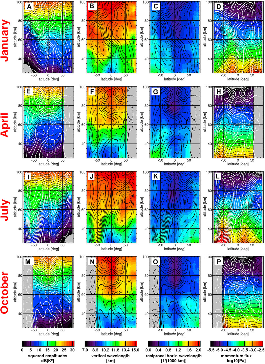
FIGURE 1. An example of application of the 2D Fourier decomposition. Using this technique, zonal averages of SABER gravity wave (A,E,I, and M) squared temperature amplitudes, (B,F,J, and N) vertical wavelengths, (C,G,K, and O) reciprocal horizontal wavelengths, and (D,H,L, and P) momentum flux absolute values for January (A,B,C, and D), April (E,F,G,and H), July (I,J,K, and L), and October (M,N,O, and P) 2006 has been measured. The overplotted contour lines are the SPARC zonal wind climatology which is arranged in an increment of 10 m/s; dashed contour lines indicate westward and solid lines are in eastward direction wind. Adapted from Figure 5: Ern et al. (2011).

2.6 Wavelet Analysis

A well-known method to retrieve gravity wave parameters from observations after background removal is the wavelet analysis (Zink and Vincent, 2001; Moldovan et al., 2002; De la Torre et al., 2006; Kramer et al., 2016; Koushik et al., 2019; Colligan et al., 2020). The procedure of the wavelet analysis technique is fully described in the work by Torrence and Compo (1998) and in the book of Nappo (2013). A detailed description of its application in the context of gravity waves is described by Zink and Vincent (2001). Regions in high wind variance in height–wavenumber spectrum are identified as gravity wave packet in their analyses.

The first step of doing a wavelet analysis is the choice of the mother wavelet (MW). Then, the Fourier transform of the MW and Fourier transform of time series data are needed to calculate a minimum scale and to choose all other scales. For each scale, computing daughter wavelet at that scale and normalizing daughter wavelet by the square root of the total wavelet variance are required. Then, multiplying by the Fourier transform of the time series and converting the transform back to the real space can visualize the dominant waves present in the observations. Generally, for analysis, one may use a Morlet wavelet because horizontal perturbations of any wind profiles caused by gravity wave packets are primarily amplitude modulated sine functions (Zink and Vincent, 2001). The wavelet transform of an arbitrary signal at space f(x) can be defined as (Moldovan et al., 2002):

$W_{\psi }\left(f\right)\left(p,q\right)=\frac{1}{\sqrt{p}}{\int }_{-\infty }^{\infty }f\left(x\right)\psi \left(\frac{x-q}{p}\right)dx,(3)$

where ψ(x) is the basis wavelet, p is called the dilation or compression scale factor, and q represents the translation at space.

Morlet wavelet can be defined as:

$\psi \left(\frac{x-q}{p}\right)=\frac{1}{\sqrt{2\pi p}}{e}^{-\frac{{\left(x-q\right)}^2}{2p^2}}{e}^{\left(\frac{i{\omega }_0\left(x-q\right)}{p}\right)},(4)$

where ω₀ denotes angular frequency of the wavelet. When q is known in this equation, p can be inferred from the local wavelength and the wavelet transform would have the maximum amplitude (Torresani, 1995).

2.6.1 Stockwell or S-Transform

This is a spectral analysis technique, similar to the continuous Gaussian wavelet analysis. Alexander et al. (2008) and Wright et al. (2010) applied the S-transform to temperature perturbations in analyzing the background of the observations by HIRDLS/Aura. Sinusoidal functions modulated with a Gaussian width inversely proportional to the wavelengths form the basis of an S-transform. Fourier transform may be obtained by the spatial integral of the S-transform. Gaussian is translated in a way that it can provide localized information of spectra (Alexander et al., 2008). Wang et al. (2006) provided detailed mathematical analysis and used a combination of S-transform and hodograph analysis for estimating gravity wave horizontal propagation directions.

2.7 Maximum Entropy Method/Harmonic Analysis

The MEM/HA method is also applicable only after the background removal and has extensively been used in a number of studies by Eckermann and Preusse (1999); Preusse et al. (2000, 2001a,b); and Ern et al. (2004, 2011, 2015).

MEM/HA is a combination of maximum entropy method [more details of MEM can be found in the work by Press and Teukolsky (1992)] and harmonic analysis, which contain certain advantages compared with the Fourier decomposition and the standard deviation, and is well suited for studying a single monochromatic wave of arbitrary wavelength from retrieved temperature (Ern et al., 2016). This technique is useful to obtain the height profiles of the amplitudes, phases, and vertical wavelengths of the two largest oscillations present in any given pair profiles of temperature (Preusse et al., 2001a). A detailed study of the method can be found in the work by Preusse et al. (2002). By following this technique and using CRISTA retrieved Kalman detrended background temperature, vertical wavelengths of 3–5 km had been detected and large GW amplitudes were found over the southernmost part of South America. This method obeys the dispersion relation for the linear 2D mountain waves. We show an example of MEM/HA analysis in Figure 2 adapted from this study. A dominant peak of vertical wavelength was found at 5 km (right panel–bottom to top vertical lines) and at 10 km.

FIGURE 2

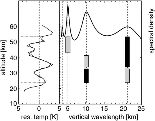
FIGURE 2. An example of MEM/HA technique applied on temperature profile observed by CRISTA 1 over Chili at 24⁰S and 82⁰W. Left panel is showing altitude profile Kalman detrended temperature residual (solid) and reconstructed fit (dash). Right panel is showing MEM spectrum, spectral peaks (bottom to top vertical lines) and two leading amplitudes (solid and hatched bars). Adapted from Figure 10: Preusse et al. (2002).

2.8 Stokes Parameter Analysis

Historically, Vincent and Fritts (1987) utilized Stokes parameters for the first time in the context of atmospheric gravity waves. By utilizing vector wind radar observations over the region of Adelaide during the period of November 1983 to December 1984, they calculated GW motions and all four Stokes parameters directly or indirectly. Stokes parameter analysis for GWs are generally done in wavenumber domain, not in height domain, because all the parameters can be extended in the Fourier spectral domain (Eckermann and Vincent, 1989). Horizontal velocity fluctuations should be polarized for gravity waves. When the analysis is done in Fourier spectral domain, one may decompose the waves at some extent. Additionally, cross spectral relationship between the zonal component and potential temperature may be established by Stokes parameter analysis (Cho et al., 1999). Stokes parameters were developed originally to explain the state of polarization of plain electromagnetic waves (EM waves) by G. G. Stokes in 1852 (Jackson, 1999). The gravity wave field may be partially polarized which triggers information retrieval by Stokes parameter analysis analogously as GWs are considered plain transverse waves, moving horizontally or vertically in nature (Colligan et al., 2020). The use of Stokes parameters can provide the polarization relations of GWs similar to EM waves and calculate the horizontal propagation direction of waves which is related to wind perturbation hodograph axial ratio (Vincent and Fritts, 1987; Eckermann and Hocking, 1989; Zink and Vincent, 2001; Wang et al., 2005; Colligan et al., 2020). There might be one way to check the presence of coherent waves in the calculation by the measurement of degree of polarization which can be calculated by using Stokes parameter analysis (Vincent and Joan Alexander, 2000).

2.9 Other Methods

There are other methods including the harmonic analysis, bispectral analysis, rotary spectral analysis, hodograph analysis, and radars. The harmonic analysis is a branch of mathematics where the representation of superposition of basic waves is discussed by the employment of Fourier series and Fourier transforms. As in the real atmosphere, GWs exist as a superposition with other large scale waves; the harmonic analysis technique is useful in tidal analysis or gravity wave analysis to characterize wave frequency. The bispectral analysis is helpful to explain nonlinear resonant wave–wave interactions (Wüst and Bittner, 2006). The rotary spectral technique (Vincent, 1984) or Hodograph analysis (Hirota and Niki, 1985) is popular to characterize the inertia gravity wave intrinsic frequency and propagation direction, though it demands the presence of a single coherent wave source and does not yield good results at the mixture of different frequencies present in the perturbation profiles (Dutta et al., 2017). In general, in a plot of fluctuation components of winds, an ellipse would be fit and the rotational direction of the ellipse would decide the propagation direction of waves. Clockwise ellipse with height in the Northern Hemisphere and anticlockwise in the Southern Hemisphere indicates upward propagation. Nevertheless, in the presence of multiple wave events, the gravity wave parameters calculated by using this method might be inaccurate as similar features could arise by superposition of linearly polarized waves in a broad spectrum (Eckermann and Hocking, 1989).

Radars have been used extensively in the stratosphere, mesosphere, and the lower thermosphere (Fritts and Alexander, 2003). Combined observation of a lidar and an MST radar at Aberystwyth (52.4°N, 4.1°W) to investigate gravity waves between 2- and 50-km revealed a dominance of long period quasi-monochromatic motions in the stratospheric gravity wave field, although this picture is not the same for the troposphere (Mitchell et al., 1994). Fritts et al. (1992) used the Jicamarca MST radar near Lima, Peru (12°S, 77°W), to understand the dynamics of equatorial mesosphere during June and August 1987, and found a very active wave field with considerable gravity wave and tidal motions with periods of ∼ 5 min to many hours (less than 1 day). Wang and Fritts (1990) used an MST radar at Poker Flat, Alaska (65°N, 147°W), to measure mesospheric GW momentum fluxes by analyzing the velocity data during the winter, summer, and fall of 1986. They showed that the wave field in the high-latitude mesosphere is highly variable. A radar at Arecibo, Puerto Rico (18°N, 67°W), and an MU radar at Shigaraki, Japan (35°N, 136°E), were used by Tsuda et al. (1989) to measure the saturated gravity wave spectrum. Meteor radar is a relatively inexpensive tool to conduct research in the upper mesosphere and lower thermosphere neutral wind fields by utilizing the reflection of electromagnetic waves from meteor trails in the range of 80–100 km altitude (Avery, 1990). Fritts et al. (2010) tested the SAAMER (The Southern Argentina Agile Meteor Radar) at Rio Grande on Tierra del Fuego (53.8°S, 67.8°W) installed in May 2008 to measure gravity wave momentum fluxes and their application at different seasons. Pramitha et al. (2019) evaluated gravity wave momentum fluxes by using three meteor radar at equatorial and low latitudes, that is, at Thumba (8.5°N, 77°E; 2006–2015), Kototabang (0.2°S, 100.3°E; 2002–2017), and Tirupati (13.63°N, 79.4°E; 2013–2018), respectively.

3 Conclusion

The objective of observations is to provide an accurate picture of the real world, which is needed to validate and improve global models of the atmosphere and gravity waves. On the other hand, improved models can help with the interpretation of observations. Also, data assimilation heavily relies on observations of atmospheric field variables. A number of techniques are used to extract GWs from observations. Briefly, two main challenges of GW retrievals are noteworthy. First, the mean field has to be adequately determined so that the fluctuating component of the atmosphere is evaluated. Second, since a broad spectrum of internal waves contributes to atmospheric fluctuations, the contribution of GWs has to be extracted carefully. It is well known from theory and observations that not only gravity waves but also acoustic (infrasonic) waves exist in the atmosphere. These listed waves differ significantly in the limiting cases of low-frequency and high-frequency waves. However, in the intermediate range, it is difficult to distinguish between them. Overall, there are different ways of retrieving GW activity from observations, depending on the nature of observations. More systematic analyses of the intercomparison of the observational retrieval techniques are needed in order to adequately evaluate the weaknesses and strengths of the different approaches. This mini review has presented some of the existing techniques of extracting GWs from atmospheric observations. We have not attempted to provide a detailed mathematical analysis; however, we have reviewed various examples of the applications of the different techniques in order to provide an exposure to the subject of GW analysis.

Author Contributions

MS and EY planned and outlined the manuscript; MS researched and wrote the manuscript. EY checked and edited the entire paper content and contributed significantly to all the sections of the paper.

Funding

MS is supported by NSF award 1849014, EY is partially funded by NASA grant 80NSSC20K0941.

Conflict of Interest

The authors declare that the research was conducted in the absence of any commercial or financial relationships that could be construed as a potential conflict of interest.

Publisher’s Note

All claims expressed in this article are solely those of the authors and do not necessarily represent those of their affiliated organizations, or those of the publisher, the editors, and the reviewers. Any product that may be evaluated in this article, or claim that may be made by its manufacturer, is not guaranteed or endorsed by the publisher.

Acknowledgments

MS thanks EY and the Department of Physics and Astronomy, George Mason University, Fairfax, VA, USA, for their wonderful support.

References

Alexander, M., Gille, J., Cavanaugh, C., Coffey, M., Craig, C., Eden, T., et al. (2008). Global Estimates of Gravity Wave Momentum Flux from High Resolution Dynamics Limb Sounder Observations. J. Geophys. Res. Atmospheres 113, 1. doi:10.1029/2007jd008807

CrossRef Full Text | Google Scholar

Allen, S. J., and Vincent, R. A. (1995). Gravity Wave Activity in the Lower Atmosphere: Seasonal and Latitudinal Variations. J. Geophys. Res. 100, 1327–1350. doi:10.1029/94jd02688

CrossRef Full Text | Google Scholar

Ando, H., Imamura, T., and Tsuda, T. (2012). Vertical Wavenumber Spectra of Gravity Waves in the Martian Atmosphere Obtained from mars Global Surveyor Radio Occultation Data. J. Atmos. Sci. 69, 2906–2912. doi:10.1175/jas-d-11-0339.1

CrossRef Full Text | Google Scholar

Avery, S. K. (1990). The Meteor Radar as a Tool for Upper Atmosphere Research. Adv. Space Res. 10, 193–200. doi:10.1016/0273-1177(90)90031-t

CrossRef Full Text | Google Scholar

Cho, J. Y. N., Newell, R. E., and Barrick, J. D. (1999). Horizontal Wavenumber Spectra of Winds, Temperature, and Trace Gases during the pacific Exploratory Missions: 2. Gravity Waves, Quasi-Two-Dimensional Turbulence, and Vortical Modes. J. Geophys. Res. 104, 16297–16308. doi:10.1029/1999jd900068

CrossRef Full Text | Google Scholar

Colligan, T., Fowler, J., Godfrey, J., and Spangrude, C. (2020). Detection of Stratospheric Gravity Waves Induced by the Total Solar Eclipse of July 2, 2019. Sci. Rep. 10, 19428–8. doi:10.1038/s41598-020-75098-2

PubMed Abstract | CrossRef Full Text | Google Scholar

Creasey, J. E., Forbes, J. M., and Hinson, D. P. (2006). Global and Seasonal Distribution of Gravity Wave Activity in mars’ Lower Atmosphere Derived from Mgs Radio Occultation Data. Geophys. Res. Lett. 33, 1. doi:10.1029/2005gl024037

CrossRef Full Text | Google Scholar

De la Torre, A., Alexander, P., Llamedo, P., Menéndez, C., Schmidt, T., and Wickert, J. (2006). Gravity Waves above the andes Detected from Gps Radio Occultation Temperature Profiles: Jet Mechanism? Geophys. Res. Lett. 33, 1. doi:10.1029/2006gl027343

CrossRef Full Text | Google Scholar

Dutta, G., Vinay Kumar, P., and Mohammad, S. (2017). Retrieving Characteristics of Inertia Gravity Wave Parameters with Least Uncertainties Using the Hodograph Method. Atmos. Chem. Phys. 17, 14811–14819. doi:10.5194/acp-17-14811-2017

CrossRef Full Text | Google Scholar

Eckermann, S. D., Hirota, I., and Hocking, W. K. (1995). Gravity Wave and Equatorial Wave Morphology of the Stratosphere Derived from Long-Term Rocket Soundings. Q.J R. Met. Soc. 121, 149–186. doi:10.1002/qj.49712152108

CrossRef Full Text | Google Scholar

Eckermann, S. D., and Hocking, W. K. (1989). Effect of Superposition on Measurements of Atmospheric Gravity Waves: A Cautionary Note and Some Reinterpretations. J. Geophys. Res. 94, 6333–6339. doi:10.1029/jd094id05p06333

CrossRef Full Text | Google Scholar

Eckermann, S. D., and Preusse, a. P. (1999). Global Measurements of Stratospheric Mountain Waves from Space. Science 286, 1534–1537. doi:10.1126/science.286.5444.1534

PubMed Abstract | CrossRef Full Text | Google Scholar

Eckermann, S. D., and Vincent, R. A. (1989). Falling Sphere Observations of Anisotropic Gravity Wave Motions in the Upper Stratosphere over australia. Pageoph 130, 509–532. doi:10.1007/bf00874472

CrossRef Full Text | Google Scholar

England, S. L., Liu, G., Yiğit, E., Mahaffy, P. R., Elrod, M., Benna, M., et al. (2017). Maven Ngims Observations of Atmospheric Gravity Waves in the Martian Thermosphere. J. Geophys. Res. Space Phys. 122, 2310–2335. doi:10.1002/2016ja023475

CrossRef Full Text | Google Scholar

Ern, M., Cho, H.-K., Preusse, P., and Eckermann, S. D. (2009a). Properties of the Average Distribution of Equatorial Kelvin Waves Investigated with the Grograt ray Tracer. Atmos. Chem. Phys. 9, 7973–7995. doi:10.5194/acp-9-7973-2009

CrossRef Full Text | Google Scholar

Ern, M. (1993). Interpolation Asynoptischer Satellitendaten. Wuppertal: Wuppertal Univ.(BUGW). Ph.D. thesis, Diploma thesis, WU D 93-35.

Google Scholar

Ern, M., Lehmann, C., Kaufmann, M., and Riese, M. (2009b). Spectral Wave Analysis at the Mesopause from Sciamachy Airglow Data Compared to Saber Temperature Spectra. Ann. Geophys. 27, 407–416. doi:10.5194/angeo-27-407-2009

CrossRef Full Text | Google Scholar

Ern, M., Preusse, P., Alexander, M. J., and Warner, C. D. (2004). Absolute Values of Gravity Wave Momentum Flux Derived from Satellite Data. J. Geophys. Res. Atmospheres 109, 1. doi:10.1029/2004jd004752

CrossRef Full Text | Google Scholar

Ern, M., Preusse, P., Gille, J., Hepplewhite, C., Mlynczak, M., Russell, J., et al. (2011). Implications for Atmospheric Dynamics Derived from Global Observations of Gravity Wave Momentum Flux in Stratosphere and Mesosphere. J. Geophys. Res. Atmospheres 116, 1. doi:10.1029/2011jd015821

CrossRef Full Text | Google Scholar

Ern, M., Preusse, P., Krebsbach, M., Mlynczak, M. G., and Russell, J. M. (2008). Equatorial Wave Analysis from Saber and Ecmwf Temperatures. Atmos. Chem. Phys. 8, 845–869. doi:10.5194/acp-8-845-2008

CrossRef Full Text | Google Scholar

Ern, M., Preusse, P., and Riese, M. (2015). Driving of the Sao by Gravity Waves as Observed from Satellite. Ann. Geophys. 33, 483–504. doi:10.5194/angeo-33-483-2015

CrossRef Full Text | Google Scholar

Ern, M., Preusse, P., and Warner, C. D. (2006). Some Experimental Constraints for Spectral Parameters Used in the warner and Mcintyre Gravity Wave Parameterization Scheme. Atmos. Chem. Phys. 6, 4361–4381. doi:10.5194/acp-6-4361-2006

CrossRef Full Text | Google Scholar

Ern, M., Trinh, Q. T., Kaufmann, M., Krisch, I., Preusse, P., Ungermann, J., et al. (2016). Satellite Observations of Middle Atmosphere Gravity Wave Absolute Momentum Flux and of its Vertical Gradient during Recent Stratospheric Warmings. Atmos. Chem. Phys. 16, 9983–10019. doi:10.5194/acp-16-9983-2016

CrossRef Full Text | Google Scholar

Fetzer, E. J., and Gille, J. C. (1994). Gravity Wave Variance in Lims Temperatures. Part I: Variability and Comparison with Background Winds. J. Atmos. Sci. 51, 2461–2483. doi:10.1175/1520-0469(1994)051<2461:gwvilt>2.0.co;2

CrossRef Full Text | Google Scholar

Fritts, D. C., and Alexander, M. J. (2003). Gravity Wave Dynamics and Effects in the Middle Atmosphere. Rev. Geophys. 41. doi:10.1029/2001rg000106

CrossRef Full Text | Google Scholar

Fritts, D. C., Yuan, L., Hitchman, M. H., Coy, L., Kudeki, E., and Woodman, R. F. (1992). Dynamics of the Equatorial Mesosphere Observed Using the Jicamarca Mst Radar during June and August 1987. J. Atmos. Sci. 49, 2353–2371. doi:10.1175/1520-0469(1992)049<2353:dotemo>2.0.co;2

CrossRef Full Text | Google Scholar

Fritts, D., Janches, D., and Hocking, W. (2010). Southern argentina Agile Meteor Radar: Initial Assessment of Gravity Wave Momentum Fluxes. J. Geophys. Res. Atmospheres 115, 1. doi:10.1029/2010jd013891

CrossRef Full Text | Google Scholar

Garcia, R. R., Lieberman, R., Russell, J. M., and Mlynczak, M. G. (2005). Large-scale Waves in the Mesosphere and Lower Thermosphere Observed by Saber. J. Atmos. Sci. 62, 4384–4399. doi:10.1175/jas3612.1

CrossRef Full Text | Google Scholar

Gavrilov, N. M., and Kshevetskii, S. P. (2015). Dynamical and thermal Effects of Nonsteady Nonlinear Acoustic-Gravity Waves Propagating from Tropospheric Sources to the Upper Atmosphere. Adv. Space Res. 56, 1833–1843. doi:10.1016/j.asr.2015.01.033

CrossRef Full Text | Google Scholar

Guest, F. M., Reeder, M. J., Marks, C. J., and Karoly, D. J. (2000). Inertia-Gravity Waves Observed in the Lower Stratosphere over Macquarie Island. J. Atmos. Sci. 57, 737–752. doi:10.1175/1520-0469(2000)057<0737:igwoit>2.0.co;2

CrossRef Full Text | Google Scholar

He, Y., Sheng, Z., Zhang, J., He, M., and Zhou, S. (2020). Spectrum Analysis of Gravity Waves Based on Sensors Mounted on a New Round-Trip Airborne Flat-Floating Sounding System. Sensors 20, 2123. doi:10.3390/s20072123

PubMed Abstract | CrossRef Full Text | Google Scholar

Heale, C. J., Snively, J. B., and Hickey, M. P. (2014). Numerical Simulation of the Long-Range Propagation of Gravity Wave Packets at High Latitudes. J. Geophys. Res. Atmos. 119, 11,116–11,134. doi:10.1002/2014JD022099

CrossRef Full Text | Google Scholar

Hickey, M., Walterscheid, R., and Schubert, G. (2011). Gravity Wave Heating and Cooling of the Thermosphere: Sensible Heat Flux and Viscous Flux of Kinetic Energy. J. Geophys. Res. Space Phys. 116, 1. doi:10.1029/2011ja016792

CrossRef Full Text | Google Scholar

Hirota, I. (1984). Climatology of Gravity Waves in the Middle Atmosphere. J. Atmos. terrestrial Phys. 46, 767–773. doi:10.1016/0021-9169(84)90057-6

CrossRef Full Text | Google Scholar

Hirota, I., and Niki, T. (1985). A Statistical Study of Inertia-Gravity Waves in the Middle Atmosphere. J. Meteorol. Soc. Jpn. 63, 1055–1066. doi:10.2151/jmsj1965.63.6_1055

CrossRef Full Text | Google Scholar

Holton, J. R., Beres, J. H., and Zhou, X. (2002). On the Vertical Scale of Gravity Waves Excited by Localized thermal Forcing. J. Atmos. Sci. 59, 2019–2023. doi:10.1175/1520-0469(2002)059<2019:otvsog>2.0.co;2

CrossRef Full Text | Google Scholar

Huang, N. E., Shen, Z., Long, S. R., Wu, M. C., Shih, H. H., Zheng, Q., et al. (1998). The Empirical Mode Decomposition and the hilbert Spectrum for Nonlinear and Non-stationary Time Series Analysis. Proc. R. Soc. Lond. A. 454, 903–995. doi:10.1098/rspa.1998.0193

CrossRef Full Text | Google Scholar

[Dataset] Jackson, J. D. (1999). Classical Electrodynamics. John Wiley & Sons.

Google Scholar

John, S. R., and Kumar, K. K. (2013). A Discussion on the Methods of Extracting Gravity Wave Perturbations from Space-Based Measurements. Geophys. Res. Lett. 40, 2406–2410. doi:10.1002/grl.50451

CrossRef Full Text | Google Scholar

John, S. R., and Kumar, K. K. (2012). Timed/saber Observations of Global Gravity Wave Climatology and Their Interannual Variability from Stratosphere to Mesosphere Lower Thermosphere. Clim. Dyn. 39, 1489–1505. doi:10.1007/s00382-012-1329-9

CrossRef Full Text | Google Scholar

Koushik, N., Kumar, K. K., Subrahmanyam, K. V., Ramkumar, G., Girach, I. A., Santosh, M., et al. (2019). Characterization of Inertia Gravity Waves and Associated Dynamics in the Lower Stratosphere over the Indian Antarctic Station, Bharati (69.4°S, 76.2°E) during Austral Summers. Clim. Dyn. 53, 2887–2903. doi:10.1007/s00382-019-04665-9

CrossRef Full Text | Google Scholar

Kramer, R., Wüst, S., and Bittner, M. (2016). Investigation of Gravity Wave Activity Based on Operational Radiosonde Data from 13 Years (1997-2009): Climatology and Possible Induced Variability. J. Atmos. Solar-Terrestrial Phys. 140, 23–33. doi:10.1016/j.jastp.2016.01.014

CrossRef Full Text | Google Scholar

Krebsbach, M., and Preusse, P. (2007). Spectral Analysis of Gravity Wave Activity in Saber Temperature Data. Geophys. Res. Lett. 34. doi:10.1029/2006gl028040

CrossRef Full Text | Google Scholar

Krisch, I., Preusse, P., Ungermann, J., Dörnbrack, A., Eckermann, S. D., Ern, M., et al. (2017). First Tomographic Observations of Gravity Waves by the Infrared Limb Imager Gloria. Atmos. Chem. Phys. 17, 14937–14953. doi:10.5194/acp-17-14937-2017

CrossRef Full Text | Google Scholar

Lait, L. R., and Stanford, J. L. (1988a). Applications of Asynoptic Space-Time Fourier Transform Methods to Scanning Satellite Measurements. J. Atmos. Sci. 45, 3784–3799. doi:10.1175/1520-0469(1988)045<3784:aoasft>2.0.co;2

CrossRef Full Text | Google Scholar

Lait, L. R., and Stanford, J. L. (1988b). Fast, Long-Lived Features in the Polar Stratosphere. J. Atmos. Sci. 45, 3800–3809. doi:10.1175/1520-0469(1988)045<3800:fllfit>2.0.co;2

CrossRef Full Text | Google Scholar

Liu, X., Yue, J., Xu, J., Wang, L., Yuan, W., Russell, J. M., et al. (2014). Gravity Wave Variations in the Polar Stratosphere and Mesosphere from Sofie/aim Temperature Observations. J. Geophys. Res. Atmos. 119, 7368–7381. doi:10.1002/2013jd021439

CrossRef Full Text | Google Scholar

Medvedev, A. S., and Yiğit, E. (2019). Gravity Waves in Planetary Atmospheres: Their Effects and Parameterization in Global Circulation Models. Atmosphere 10, 531. doi:10.3390/atmos10090531

CrossRef Full Text | Google Scholar

Meyer, C. I., Ern, M., Hoffmann, L., Trinh, Q. T., and Alexander, M. J. (2018). Intercomparison of Airs and Hirdls Stratospheric Gravity Wave Observations. Atmos. Meas. Tech. 11, 215–232. doi:10.5194/amt-11-215-2018

CrossRef Full Text | Google Scholar

Mitchell, N. J., Thomas, L., and Prichard, I. T. (1994). Gravity Waves in the Stratosphere and Troposphere Observed by Lidar and Mst Radar. J. Atmos. terrestrial Phys. 56, 939–947. doi:10.1016/0021-9169(94)90155-4

CrossRef Full Text | Google Scholar

Moldovan, H., Lott, F., and Teitelbaum, H. (2002). Wave Breaking and Critical Levels for Propagating Inertio-Gravity Waves in the Lower Stratosphere. Q. J. R. Meteorol. Soc. 128, 713–732. doi:10.1256/003590002321042162

CrossRef Full Text | Google Scholar

Nakagawa, H., Terada, N., Jain, S. K., Schneider, N. M., Montmessin, F., Yelle, R. V., et al. (2020). Vertical Propagation of Wave Perturbations in the Middle Atmosphere on mars by Maven/iuvs. J. Geophys. Res. Planets 125, e2020JE006481. doi:10.1029/2020je006481

CrossRef Full Text | Google Scholar

Nappo, C. J. (2013). An Introduction to Atmospheric Gravity Waves. Academic Press.

Google Scholar

Nayak, C., and Yiğit, E. (2019). Variation of Small‐Scale Gravity Wave Activity in the Ionosphere during the Major Sudden Stratospheric Warming Event of 2009. J. Geophys. Res. Space Phys. 124, 470–488. doi:10.1029/2018ja026048

CrossRef Full Text | Google Scholar

Pfenninger, M., Liu, A. Z., Papen, G. C., and Gardner, C. S. (1999). Gravity Wave Characteristics in the Lower Atmosphere at South Pole. J. Geophys. Res. 104, 5963–5984. doi:10.1029/98jd02705

CrossRef Full Text | Google Scholar

Pramitha, M., Kishore Kumar, K., Venkat Ratnam, M., Rao, S. V. B., and Ramkumar, G. (2019). Meteor Radar Estimations of Gravity Wave Momentum Fluxes: Evaluation Using Simulations and Observations over Three Tropical Locations. J. Geophys. Res. Space Phys. 124, 7184–7201. doi:10.1029/2019ja026510

CrossRef Full Text | Google Scholar

[Dataset] Press, W., and Teukolsky, S. (1992). Wb Numerical Recipes in C–The Art of Scientific Programming. Cambridge University Press.

Google Scholar

Preusse, P., Dörnbrack, A., Eckermann, S. D., Riese, M., Schaeler, B., Bacmeister, J. T., et al. (2002). Space-based Measurements of Stratospheric Mountain Waves by Crista 1. Sensitivity, Analysis Method, and a Case Study. J. Geophys. Res. Atmospheres 107, 6. doi:10.1029/2001jd000699

CrossRef Full Text | Google Scholar

Preusse, P., Eckermann, S. D., Oberheide, J., Hagan, M. E., and Offermann, D. (2001a). Modulation of Gravity Waves by Tides as Seen in Crista Temperatures. Adv. Space Res. 27, 1773–1778. doi:10.1016/s0273-1177(01)00336-2

CrossRef Full Text | Google Scholar

Preusse, P., Eckermann, S. D., and Offermann, D. (2000). Comparison of Global Distributions of Zonal-Mean Gravity Wave Variance Inferred from Different Satellite Instruments. Geophys. Res. Lett. 27, 3877–3880. doi:10.1029/2000gl011916

CrossRef Full Text | Google Scholar

Preusse, P., Eidmann, G., Eckermann, S. D., Schaeler, B., Spang, R., and Offermann, D. (2001b). Indications of Convectively Generated Gravity Waves in Crista Temperatures. Adv. Space Res. 27, 1653–1658. doi:10.1016/s0273-1177(01)00231-9

CrossRef Full Text | Google Scholar

Rodgers, C. D. (1977). Statistical Principles of Inversion Theory. Inversion Methods Atmos. remote sounding 3, 117–138. doi:10.1016/b978-0-12-208450-8.50010-2

CrossRef Full Text | Google Scholar

Savitzky, A., and Golay, M. J. E. (1964). Smoothing and Differentiation of Data by Simplified Least Squares Procedures. Anal. Chem. 36, 1627–1639. doi:10.1021/ac60214a047

CrossRef Full Text | Google Scholar

Torrence, C., and Compo, G. P. (1998). A Practical Guide to Wavelet Analysis. Bull. Amer. Meteorol. Soc. 79, 61–78. doi:10.1175/1520-0477(1998)079<0061:apgtwa>2.0.co;2

CrossRef Full Text | Google Scholar

Torresani, B. (1995). Position-frequency Analyis for Signals Defined on Spheres. Signal. Process. 43, 341–346. doi:10.1016/0165-1684(95)00037-e

CrossRef Full Text | Google Scholar

Tsuda, T., Inoue, T., Kato, S., Fukao, S., Fritts, D. C., and VanZandt, T. E. (1989). Mst Radar Observations of a Saturated Gravity Wave Spectrum. J. Atmos. Sci. 46, 2440–2447. doi:10.1175/1520-0469(1989)046<2440:mrooas>2.0.co;2

CrossRef Full Text | Google Scholar

Tsuda, T., Murayama, Y., Wiryosumarto, H., Harijono, S. W. B., and Kato, S. (1994). Radiosonde Observations of Equatorial Atmosphere Dynamics over indonesia: 2. Characteristics of Gravity Waves. J. Geophys. Res. 99, 10507–10516. doi:10.1029/94jd00354

CrossRef Full Text | Google Scholar

Tsuda, T., Nishida, M., Rocken, C., and Ware, R. H. (2000). A Global Morphology of Gravity Wave Activity in the Stratosphere Revealed by the Gps Occultation Data (Gps/met). J. Geophys. Res. 105, 7257–7273. doi:10.1029/1999jd901005

CrossRef Full Text | Google Scholar

Vincent, R. A., and Fritts, D. C. (1987). A Climatology of Gravity Wave Motions in the Mesopause Region at Adelaide, australia. J. Atmos. Sci. 44, 748–760. doi:10.1175/1520-0469(1987)044<0748:acogwm>2.0.co;2

CrossRef Full Text | Google Scholar

Vincent, R. A. (1984). Gravity-wave Motions in the Mesosphere. J. Atmos. terrestrial Phys. 46, 119–128. doi:10.1016/0021-9169(84)90137-5

CrossRef Full Text | Google Scholar

Vincent, R. A., and Joan Alexander, M. (2000). Gravity Waves in the Tropical Lower Stratosphere: An Observational Study of Seasonal and Interannual Variability. J. Geophys. Res. 105, 17971–17982. doi:10.1029/2000jd900196

CrossRef Full Text | Google Scholar

Wang, D.-Y., and Fritts, D. C. (1990). Mesospheric Momentum Fluxes Observed by the Mst Radar at Poker Flat, alaska. J. Atmos. Sci. 47, 1512–1521. doi:10.1175/1520-0469(1990)047<1512:mmfobt>2.0.co;2

CrossRef Full Text | Google Scholar

Wang, L., Fritts, D. C., Williams, B. P., Goldberg, R. A., Schmidlin, F. J., and Blum, U. (2006). Gravity Waves in the Middle Atmosphere during the Macwave winter Campaign: Evidence of Mountain Wave Critical Level Encounters. Ann. Geophys. 24, 1209–1226. doi:10.5194/angeo-24-1209-2006

CrossRef Full Text | Google Scholar

Wang, L., Geller, M. A., and Alexander, M. J. (2005). Spatial and Temporal Variations of Gravity Wave Parameters. Part I: Intrinsic Frequency, Wavelength, and Vertical Propagation Direction. J. Atmos. Sci. 62, 125–142. doi:10.1175/jas-3364.1

CrossRef Full Text | Google Scholar

Wang, L., and Geller, M. A. (2003). Morphology of Gravity-Wave Energy as Observed from 4 Years (1998-2001) of High Vertical Resolution U.S. Radiosonde Data. J. Geophys. Res. 108, 1. doi:10.1029/2002jd002786

CrossRef Full Text | Google Scholar

Wright, C., Osprey, S., Barnett, J., Gray, L. J., and Gille, J. (2010). High Resolution Dynamics Limb Sounder Measurements of Gravity Wave Activity in the 2006 Arctic Stratosphere. J. Geophys. Res. Atmospheres 115, 1. doi:10.1029/2009jd011858

CrossRef Full Text | Google Scholar

Wüst, S., and Bittner, M. (2006). Non-linear Resonant Wave-Wave Interaction (Triad): Case Studies Based on Rocket Data and First Application to Satellite Data. J. Atmos. solar-terrestrial Phys. 68, 959–976. doi:10.1016/j.jastp.2005.11.011

CrossRef Full Text | Google Scholar

Yamashita, C., England, S. L., Immel, T. J., and Chang, L. C. (2013). Gravity Wave Variations during Elevated Stratopause Events Using Saber Observations. J. Geophys. Res. Atmos. 118, 5287–5303. doi:10.1002/jgrd.50474

CrossRef Full Text | Google Scholar

Yiğit, E., England, S. L., Liu, G., Medvedev, A. S., Mahaffy, P. R., Kuroda, T., et al. (2015). High-altitude Gravity Waves in the Martian Thermosphere Observed by Maven/ngims and Modeled by a Gravity Wave Scheme. Geophys. Res. Lett. 42, 8993–9000.

Google Scholar

Yiğit, E., Knížová, P. K., Georgieva, K., and Ward, W. (2016). A Review of Vertical Coupling in the Atmosphere–Ionosphere System: Effects of Waves, Sudden Stratospheric Warmings, Space Weather, and of Solar Activity. J. Atmos. Solar-Terrestrial Phys. 141, 1–12.

Google Scholar

Yiğit, E., Medvedev, A. S., Aylward, A. D., Hartogh, P., and Harris, M. J. (2009). Modeling the Effects of Gravity Wave Momentum Deposition on the General Circulation above the Turbopause. J. Geophys. Res. Atmospheres 114, 1.

Google Scholar

Yiğit, E., Medvedev, A. S., and Ern, M. (2021). Effects of Latitude-dependent Gravity Wave Source Variations on the Middle and Upper Atmosphere. Front. Astron. Space Sci. 7, 1. doi:10.3389/fspas.2020.614018

CrossRef Full Text | Google Scholar

Zhang, S. D., and Yi, F. (2005). A Statistical Study of Gravity Waves from Radiosonde Observations at Wuhan (30° N, 114° E) China. Ann. Geophys. 23, 665–673. doi:10.5194/angeo-23-665-2005

CrossRef Full Text | Google Scholar

Zhang, S. D., Yi, F., Huang, C. M., and Zhou, Q. (2010). Latitudinal and Seasonal Variations of Lower Atmospheric Inertial Gravity Wave Energy Revealed by Us Radiosonde Data. Ann. Geophys. 28, 1065–1074. doi:10.5194/angeo-28-1065-2010

CrossRef Full Text | Google Scholar

Zhang, S. D., and Yi, F. (2007). Latitudinal and Seasonal Variations of Inertial Gravity Wave Activity in the Lower Atmosphere over central china. J. Geophys. Res. Atmospheres 112, 1. doi:10.1029/2006jd007487

CrossRef Full Text | Google Scholar

Zink, F., and Vincent, R. A. (2001). Wavelet Analysis of Stratospheric Gravity Wave Packets over Macquarie Island: 1. Wave Parameters. J. Geophys. Res. 106, 10275–10288. doi:10.1029/2000jd900847

CrossRef Full Text | Google Scholar