Identification and Classification of Relativistic Electron Precipitation at Earth Using Supervised Deep Learning

1 Introduction

The radiation belt environment is highly dynamic and it is governed by acceleration, transport and loss processes (e.g., Li and Hudson, 2019; Reeves et al., 2003). One of the loss mechanisms is electron precipitation (EP), which occurs when the conservation of the first adiabatic invariant is violated (e.g., Schulz and Lanzerotti, 1974; Horne and Thorne, 1998): electrons are no longer trapped by the Earth’s magnetic field and fall into the upper atmosphere. Not only electron depletion is important in the radiation belt evolution in time and flux, but electron precipitation is also known to drive many atmospheric effects related to space weather. Multiple studies have indeed associated conductivity variations and atmospheric chemistry changes (potentially leading to ozone reduction) with electron precipitation (Robinson et al., 1987; Fytterer et al., 2015; Mironova et al., 2015; Tyssøy et al., 2016; Khazanov et al., 2018; Meraner and Shmidt, 2018; Yu et al., 2018; Duderstadt et al., 2021; Sinnhuber et al., 2021).

It is well understood that electron precipitation can occur as a result of interactions between plasma waves existing in the magnetosphere and the trapped electron population in the radiation belts (e.g., Millan and Thorne, 2007; Thorne, 2010). Electrons can also be lost if the magnetic field line around which they gyrate is stretched away from Earth or undergoes a significant geometry variation such that the curvature radius of the field line is comparable to the gyroradius of the electrons (e.g., Büchner and Zelenyi, 1989; Dubyagin et al., 2021; Sergeev et al., 1983, 1993). This process is called field line curvature scattering or current sheet scattering (CSS). Under these conditions, the field line no longer traps the electrons, and these electrons can precipitate into the atmosphere. The location where precipitation occurs (called isotropic boundary, IB) depends on electron energy (Capannolo et al., 2022; Yahnin et al., 2016; 2017). This phenomenon has also been widely studied for protons (Ganushkina et al., 2005; Gilson et al., 2012; Liang et al., 2014; Dubyagin et al., 2018).

A comprehensive understanding of which mechanism (waves or CSS) dominates the electron precipitation and thus the energy input into the Earth’s atmosphere is still under active research. Given the Earth’s magnetic field geometry, one would expect that on the dayside and at low L shells CSS does not contribute much, but more quantitative studies are still needed. Overall, while wave-driven precipitation can occur at all MLT (magnetic local time) sectors, CSS-driven precipitation is indeed primarily observed over 20–04 MLT (Yahnin et al., 2016; 2017), and overlaps with precipitation driven by waves (for the most part, electromagnetic ion cyclotron waves, EMIC) in the midnight sector (Capannolo et al., 2022).

These studies use data from the constellation of satellites called POES (Polar Orbiting Environmental Satellites) and MetOp (Meteorological Operational), described in Section 2. An example of a wave-driven (REP, relativistic electron precipitation) event is shown in Figure 1A, together with an example of a CSS-driven (CSS) event (Figure 1B). REP events show enhancements in the relativistic (>700 keV) precipitating electron flux (solid red line) and the precipitation is rather isolated (gray region) in space (L shell) with little/no precipitation around the main event. This region generally matches the location where the wave-particle interaction is efficient to violate the first adiabatic invariant. CSS events, instead, show an energy-dependent precipitation with higher energy electrons precipitating at lower L shells than lower energy electrons (Figure 1B; green, black, and blue solid lines). This is a direct result from the fact that the electron gyroradius depends on electron energy: higher energy electrons have a larger gyroradius, thus are lost by a stretched magnetic field line at distances closer to Earth (smaller L shells) than lower energy electrons. Given such a distinct pattern of precipitation, we can distinguish the precipitation drivers.

FIGURE 1

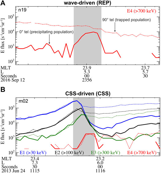
FIGURE 1. Examples of (A) a wave-driven (REP) precipitation event and (B) a CSS-driven (CSS) precipitation event. Electron flux observed by POES n19 (A) and MetOp m02 (B) satellites is color-coded by energy channel (as indicated in panel (B)), and shown as a function of time and satellite trajectory expressed in L and MLT. Dashed (solid) lines are relative to the 90° (0°) telescope, indicating the trapped (precipitating) electrons. The precipitation events are highlighted by the gray rectangles.

So far, existing analyses aiming to distinguish the precipitation drivers have either focused on a limited time span (Yahnin et al., 2016; 2017) or on a limited MLT sector (Capannolo et al., 2022). Identifying precipitation events and visually inspecting their precipitation patterns to categorize their driver (waves or CSS) is a rather time-expensive task. Algorithms that find relativistic electron precipitation events (based on count rate or flux thresholds) exist in literature (e.g., Shekhar et al., 2017; Gasque et al., 2021; Capannolo et al., 2022), but they do not include the distinction between wave-driven precipitation and CSS-driven precipitation, which is a much more complex task to perform using algorithms. The goal of this work is to take advantage of deep learning techniques not only to find precipitation events, but also to categorize them into wave-driven (REP) and CSS-driven (CSS) events. We use the dataset of precipitation events analyzed in Capannolo et al. (2022), which were visually classified between wave-driven (REPs) and CSS-driven (CSSs) precipitation events (details in Capannolo et al., 2022). This work is an example of an application of supervised deep learning classification in space sciences that is able to provide a large dataset of precipitation events classified by driver (waves or CSS) after an initial manual classification of events.

2 Satellite Data Description

We use data from the POES and MetOp network of sun-synchronous satellites in polar orbits at ∼800–850 km of altitude (Evans and Greer, 2004). The Medium Energy Proton and Electron Detector (MEPED) provides electron (and proton) flux in three integral channels with cutoff energies of >30 keV (E1), >100 keV (E2), and >300 keV (E3) (Rodger et al., 2010). The P6 proton channel is designed to measure >6.9 MeV protons, however, it is also sensitive to electrons at >700 keV (Yando et al., 2011) in absence of high energy protons. Thus, we use the P6 channel as a fourth virtual electron channel, E4 (Green, 2013). Additionally, each satellite is equipped with two telescopes: one oriented along zenith (0° telescope) and one perpendicular to it (90° telescope), both with full field-of-view angle of 30°. At mid-to-high latitudes, the 0° telescope provides measurements of electrons precipitating deep into the loss cone and the 90° telescope provides observations of trapped electrons. Strong precipitation typically occurs when the flux observed by the 0° telescope approaches the flux observed by the 90° telescope, indicating that a large percentage of trapped electrons are precipitating. Precipitation events are marked in gray in Figures 1–3, and highlighted in brown (REP) and blue (CSS) in Figure 4. The resolution of the electron flux is 2 s, and the constellation of satellite covers a rather broad L-shell range and MLT sectors. Typical observations of POES/MetOp are shown in the Supplementary Figure S1. Each panel shows ¼ orbit of a POES/MetOp satellites (one pass through the radiation belts) and highlights the significant variability of flux during the satellite trajectory.

3 Methods

In this section, we describe how we prepared the dataset of precipitation events in order to obtain a well-performing model. We also describe the model architecture and how it was decided, as well as how we trained the deep learning model.

3.1 Dataset Preparation

Capannolo et al. (2022) analyzed relativistic electron precipitation events observed by POES/MetOp from 2012 to 2020 over 22–02 MLT and classified these events between those driven by waves (called REP events in this work) from those driven by CSS (CSSs hereafter) using their characteristic precipitation profile (Figure 1). Note that this dataset was obtained after careful event classification: only events that clearly belonged to either category (REP or CSS) were considered, while ambiguous precipitation events were carefully discarded. More details on the classification are provided in Capannolo et al. (2022). In this work, we use this dataset of precipitation events classified over 22–02 MLT with additional preprocessing to improve the model performance as explained below.

Our goal is to build a dataset of precipitation events randomly stacked one after the other. We consider all four POES/MetOp electron channels and the two look directions (0° and 90°) for a total of eight inputs at a given time. The model output (or target) is the data point class (or label, used interchangeably hereafter): 0 is for no-event, 1 is for REP, and 2 is for CSS. Given one event, the data points are labeled as 1 or 2 during the precipitation (gray regions of Figure 1) and the adjacent data points (to the left and right of the event) are labeled with 0. Fluxes ≤0 for all channels are set to 0.01 (100) s⁻¹cm⁻²sr⁻¹ for the 0° (90°) telescope measurements (negative values in POES/MetOp data indicate unreliable flux measurements). We apply the natural logarithm to the fluxes and normalize the whole dataset using the normalization parameters of the train dataset.

As shown in Supplementary Figure S1, each pass through the radiation belts highlights a significant flux variability observed by POES/MetOp, while the precipitation events are rather short-lived (<30–60 s). As a result, if we use the full day of data when a given REP/CSS event occurs, we will obtain a label of mostly zeroes (no-event) and only a few data points at 1 or 2 (indicating the REP/CSS). This would make the full dataset of stacked events extremely imbalanced, where only a few percent of the labels are non-zero. With such dataset, the deep learning model is unable to perform well and it identifies only the no-events correctly. In order to overcome this obstacle, we consider a much shorter window of data for each event: given one event, we label the data points during precipitation with 1 or 2, but label with 0 only the data points adjacent to the left and right of the event such that the total number of data points is 50. In this way, we have windows of 50-point-long for each event which we stack one after the other in a random order. Additionally, we ensure that no other nearby events were occurring within the 50-point-long window such that in this window there is only one type of non-zero label (either 1 or 2). Note that if two events of different classes are adjacent to each other, we rule out both. Instead, if two REP events are adjacent to each other within the 50-point-long window, we widen the label of one to include both to ensure that in each 50-point-long window, there is only one continuous non-zero label. For the CSS events, we also manually extended the boundary of the precipitation events to include the full energy dispersion observed by POES/MetOp because we do not limit ourselves to the E4 precipitation alone (as done in Capannolo et al., 2022). This ensures that the full precipitation pattern (from low to high electron energy) is identified as a CSS event and used to train the model. Using the boundaries as in Capannolo et al. (2022) worsens the model performance because the full extent of the energy-dependent pattern is not correctly learned by the model. We show a portion of the dataset in Figure 2: panel A) indicates the label and panel B) shows the electron flux for all energy channels and look directions, where the precipitation events are highlighted in gray.

FIGURE 2

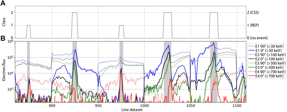
FIGURE 2. Portion of the training dataset: (A) class of each data point and b) electron flux for different energies. Dashed and solid lines in panel (B) indicate the 90° and 0° telescope observations, respectively, as in Figure 1. Precipitation events are highlighted in gray in panel (B) and their relative class is shown in panel (A), where class 0 indicates “no event”, class 1 indicates “REP event” and class 2 indicates “CSS event”.

In order to augment our dataset and provide the model with a wider variety of precipitation patterns, we also mirror each precipitation event about its main axis. This does not introduce data redundancy since each precipitation event (either mirrored or not) carries a meaningful information. In other words, a REP/CSS event can be directly observed by a POES/MetOp satellite following its actual trajectory (e.g., from low to high L shells), but the precipitation pattern would still be observed (though symmetrically) if the same POES/MetOp satellite was travelling along its opposite orbit (e.g., from high to low L shells) through the precipitation region at the same time. Note that this is possible since we are only interested in the profile of the precipitation (i.e., flux evolution as a function of dataset index) and not its temporal evolution. By using this methodology, we obtain a dataset of 460 REPs and 348 CSSs for a total dataset length of 40,400 data points. Although only ∼20% of the data points are labeled with 1 or 2 (making this dataset still imbalanced with respect to the 0 class), the REP and CSS classes are approximately balanced (∼10% data points are REPs and ∼8% data points are CSSs) and the model is able to identify correctly no-events, REPs and CSSs as we show in the following sub-sections.

3.2 Model Structure and Training

We adapt a long short-term memory (LSTM; Hochreiter and Schmidhuber, 1997) architecture (a type of artificial recurrent neural network, RNN; Rumelhart et al., 1986) for the deep learning model because it retains input information at much earlier time steps, making it more efficiently than RNNs for problems that treat time series. As a matter of fact, the problem of our work is a time series classification. Although the time variable is not explicitly used, it is instead intrinsically represented by the shape of the precipitation. It is indeed the evolution of the precipitation pattern (isolated vs energy-dependent) that differentiates between the two drivers of precipitation, as mentioned in Section 1.

The input format required by LSTM is a tensor, which is composed of a stack of snapshots of the dataset identified by a sliding window with stride one and length 7. The label in each snapshot is assigned as the most probable one (i.e., if the majority of data points have label of 0, the label assigned to that snapshot is also 0) and is one-hot encoded. The length of seven is set after trying different sliding window lengths and choosing the one that provided the best model performance.

The metrics we use are those of a standard classification problem and we focus on the F1 score (calculated as the weighted average of the precision and recall; it expresses how many events the classifier identifies correctly quantifying also how many are missed or mislabeled), the AUC (area under the ROC (Receiver Operating Characteristic) recall vs false-positive-rate curve) and the AUPRC (area under the precision vs. recall curve). We perform a k-fold cross validation with k = 10: the whole dataset is split into 10 portions of which one is used as a test set and the remaining nine are used as training set. We also consider a validation set that is 15% of the training set in each k-fold. The k-fold cross validation consists in training the model on k different datasets (described above) and estimating the model performance for each of the k iterations. The final model performance is the average of the k performances and the final model weights are obtained by training the model on the whole dataset (with the exception of 15% of the dataset used for testing purposes). During training, we use early stopping (with patience of 10 epochs) on the AUC calculated for the validation dataset.

4 Model Performance

We tried different model configurations, all made of a LSTM layer followed by a fully connected (i.e., dense) layer, ending with a dense layer of three neurons that outputs one predicted class. There are two dropout layers (with 0.5 dropout rate) after the LSTM layer and after the first dense layer. We validated each model configuration using the k-fold cross-validation (mentioned above) and we selected the model configuration with the highest F1 score, AUC and AUPRC. Out of all the configurations we tried (64 LSTM cells + 256 dense cells; 128 LSTM cells + 128 dense cells; 128 LSTM cells + 256 dense cells; 64 bidirectional LSTM cells + 256 dense cells; 64 bidirectional LSTM cells + 64 bidirectional LSTM cells + 128 dense cells) the model with the best performance is the one with a layer of 64 bidirectional LSTM cells followed by a fully connected layer of 256 cells (total number of free parameters is 71,171). The metrics resulting from the k-fold cross-validation for this model are: F1∼0.948, AUC∼0.995, and AUPRC∼0.990. Note that the performance among the different model configurations is similar and differs only on the second or third decimal figure. Supplementary Table S1 shows the performance scores (F1, AUC, AUPRC) resulting from the k-fold cross-validation for each architecture tested. As an example, Supplementary Figure S2 (panels a–e) shows the metrics as a function of epoch for the k = 3 fold. Panel f) shows the confusion matrix averaged from all the confusion matrices of each k-fold: the highest values are focused along the diagonal, indicating that the model performs well in assigning the correct class to each snapshot.

To highlight that the model appropriately identifies and classifies precipitation events, we show in Figure 3 three examples of how the model performs on three portions of the test dataset. Panels A), C), and E) present the model (solid) and original (dashed) labels and panels B), D), F) show the electron fluxes in a similar format as Figure 2. The precipitation events (originally assigned) are highlighted in gray and their associated class is reported in the panels A), C), E). Not only the model identifies all precipitation events, but each event is categorized in the class originally assigned. Note that the indices where the labels are non-zero only indicate that nearby that region the probability of finding an event is higher than the probability of a no-event, but these indices do not necessarily represent the exact precipitation event boundaries (as the original class does). Nevertheless, the labels predicted by the model are in good agreement with the original location and class of the events highlighted in gray. The model labels seem to be shifted to the left by a few data points compared to the original classes, due to the fact that we assign a class to each snapshot of length 7 (described in Section 3.1). In other words, the very first snapshot is classified with the most probable label in the first seven data points. As the sliding window progresses with stride 1, each label is associated with the following seven data points resulting in anticipating the snapshot classification.

FIGURE 3

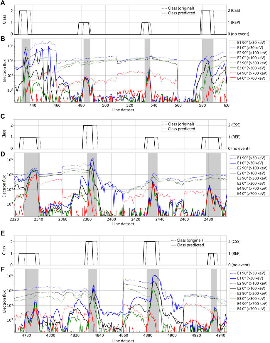
FIGURE 3. Three different portions of the test dataset in a similar format as Figure 2. Panels (A), (C) and (E) show the original class of each event in the dashed gray line and the class of each event predicted by the model in solid black. Panels (B), (D) and (F) show the electron flux in a similar format as Figure 2B, where each event (originally identified) is highlighted in gray.

4.1 Model Application on Several Days of POES/MetOp Data: Preliminary Results

As we showed in Section 3.1, the dataset used for training has been significantly shrunk to only 50 data points for each precipitation event observed by POES/MetOp. In this section, we explore the model performance on longer time periods (full day of POES/MetOp data, the significant flux variability of which is shown in Supplementary Figure S1 to test its generalization ability.

We apply the model to several POES/MetOp days and show the results in Figure 4 and Supplementary Figure S3. Each panel in these figures is from a different date and none of the events shown belong to the dataset prepared in Section 3.1 (they are all out-of-sample). Here, we are only considering events occurring in the outer radiation belt, thus we filter out any events occurring at L < 2.5 or L > 8.5 (L is expressed using the International Geomagnetic Reference Field, IGRF, model in POES/MetOp data). The panels on the left column of Figure 4 show REP events (highlighted in brown), whereas the events on the right column are CSSs (highlighted in blue). This classification is accurate because the classified REPs indeed show isolated E4 precipitation, while the classified CSSs display an energy-dependent precipitation. During REP events (Figures 2–4), although the low-energy electrons (E1, E2 and E3 channels) appear to precipitate as well, their flux is likely the result of proton contamination, which is known to affect the electron measurements onboard POES/MetOp satellites (e.g., Evans and Greer, 2004; Yando et al., 2011; Capannolo et al. 2019, 2021). Note again that the location where these events are identified by the model differs from the exact event location by a few data points. This is not a major concern as this shift appears to be systematic and can be corrected in the post-processing by shifting the predicted model class by a few data points.

FIGURE 4

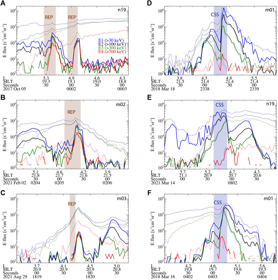
FIGURE 4. Identification and classification of precipitation events on 6 days of POES/MetOp data. Each panel shows the electron flux color-coded in energy (legend in panel (A)) as a function of L, MLT, and time. Dashed (solid) lines indicate observations of trapped (precipitating) electrons from the 90° (0°) telescope. REP events identified by the model are highlighted in brown, while CSS events identified by the model are marked in blue.

On the contrary, Supplementary Figure S3 shows examples when the model does not perform very well and identifies two adjacent precipitation events belonging to different classes (panels a and b), mislabeled events (panel c) or false positive events (panel d). The cases in panel a) only last one data point and could be potentially disregarded since the model does not identify a long enough non-zero label. The event in panel d) shows a precipitating E4 flux that is higher than the others, which could indicate a potential issue in the recorded POES/MetOp data. Events in panels b) and c) instead must be appropriately ruled out or inspected further (e.g., what is the probability of each class? Is the probability of the CSS class comparable to that of the REP?). Handling false positives is beyond the scope of this work and we are aware that post-processing on the model output is needed before using these results for scientific research. The post-processing should rule out events lasting only one data point, adjacent events belonging to different non-zero classes, and events in the South Atlantic Anomaly, as well as improving the L shell calculation for each event (using Tsyganenko models such as the T89 (Tsyganenko, 1989) or T05 (Tsyganenko and Sitnov, 2005)) used to consider events occurring only in the outer radiation belt.

5 Conclusions and Discussion

In this work, we showed an example of an application of supervised deep learning to space sciences. Understanding when, where and why relativistic electrons precipitate into the Earth’s atmosphere has a longstanding relevance for a variety of reasons (from improving our knowledge on plasma dynamics to study the space weather impacts of electron precipitation). In this work, we focused specifically on relativistic electron precipitation. Our goal was to classify the relativistic electron precipitation events depending on their spatial precipitation pattern, which in turn corresponds to their magnetospheric driver (waves or current sheet scattering). We used data from the POES/MetOp constellation of low-Earth-orbit satellites. Our task was supervised because we used the list of events studied by Capannolo et al. (2022), which were visually classified. Note that these events were classified only in a limited MLT sector (22–02); however, their MLT value was not used as input in the model, and in fact, our model is able to identify precipitation events at any MLT.

The dataset preparation was key to obtain a satisfying model performance. By considering only a short time window around each event instead of the full day of POES/MetOp data, using non-zero labels to indicate REPs (class of 1) or CSSs (class of 2) and labels at 0 to indicate the no-event, and including electron fluxes observed at different energies and look directions, we were able to obtain an appropriate dataset to use for training. We found that the LSTM architecture is suitable for identifying precipitation events and classifying them by precipitation pattern given its ability to consider the data history (in our case the precipitation pattern profile evolution along the satellite trajectory).

Our model is composed of one layer of 64 bidirectional LSTM cells, one layer of 256 fully connected neurons, and one layer of three dense cells. The inputs are the electron fluxes at different energies and look directions, and the output is the class of each data point. We obtained the model metrics (F1∼0.948, AUC∼0.995, and AUPRC∼0.990) by conducting a k-fold cross-validation (k = 10). Our model is able to learn the dataset properties correctly. The model is not only able to identify the electron precipitation events, but it also appropriately classifies them by their drivers.

Since the dataset used for training and testing purposes has been specifically designed to obtain a good model performance, it shows less variability than that typically observed by POES/MetOp over an entire orbit. Nevertheless, our model is still able to identify and classify the precipitation events when applied to a full day of data (Figure 4), though some false positives might still be identified (Supplementary Figure S3). Post-processing of these results is needed before being able to use the model outputs for scientific research; however, this is beyond the scope of this paper and left for future investigation. Once the post-processing routine is developed, this model could be easily used as a tool to produce lists of relativistic electron precipitation events in a very short amount of time, overcoming the complex task of developing deterministic algorithms based on flux thresholds to delineate the precipitation patterns and the time-expensive task of visually classifying these events by driver. In this way, we would be able to extend the study conducted in Capannolo et al. (2022) to the whole MLT range and statistically investigate on where the CSS effects should be considered for radiation belt and precipitation modeling, as well as compare them with the precipitation driven by waves. Such event dataset would also potentially open additional avenues of machine learning applications to space sciences; for example, from a space weather point of view, we could investigate if the electron precipitation events can be predicted by using solar images, solar wind data and/or geomagnetic indices.

Data Availability Statement

Publicly available datasets were analyzed in this study. This data can be found here: https://satdat.ngdc.noaa.gov/sem/poes/data/processed/ngdc/uncorrected/full/. The dataset preparation and model training are done on a Linux OS (version 3.10.0-1160.49.1.el7.x86_64) machine (Shared Computer Cluster at Boston University) in Python (version 3.8.6), using the TensorFlow library (version 2.5.0, https://www.tensorflow.org) and the Python packages: Matplotlib (https://matplotlib.org), Scikit Learn (https://scikit-learn.org/stable/), Xarray (https://xarray.pydata.org/en/stable/), Joblib (https://joblib.readthedocs.io/en/latest/), Seaborn (https://seaborn.pydata.org/), Numpy (https://numpy.org), and Pandas (https://pandas.pydata.org). Figures 1,4 and Supplementary Figures S1,S3 have been produced in IDL (version 8.6.0). The trained model and a sample Python script to apply the model on any POES/MetOp date can be found in the GitHub repository here: https://github.com/luisacap/REPs_classifier_codes_for_paper.git.

Author Contributions

LC conducted the core of this work (dataset preparation, model development, model training, etc.). WL and SH contributed equally by offering feedback during the preparation of this work, and they share the last authorship.

Funding

This research is supported by the NSF grants AGS-1723588 and AGS-2019950, the NASA grants 80NSSC20K0698 and 80NSSC20K1270, and the Alfred P. Sloan Research Fellowship FG-2018-10936. SH would like to acknowledge the NASA FINESST Award 80NSSC21K1385.

Conflict of Interest

The authors declare that the research was conducted in the absence of any commercial or financial relationships that could be construed as a potential conflict of interest.

Publisher’s Note

All claims expressed in this article are solely those of the authors and do not necessarily represent those of their affiliated organizations, or those of the publisher, the editors and the reviewers. Any product that may be evaluated in this article, or claim that may be made by its manufacturer, is not guaranteed or endorsed by the publisher.

Acknowledgments

LC would like to acknowledge M. Capannolo for the insightful conversations on machine and deep learning. LC also acknowledges her teammates in the 2020 Heliophysics hackweek (B. Tremblay, A. K. Tiwari, A. Hu, B. Thompson, S. Shekhar, M. Shumko, S. Forsyth, J. Li, and D. Linko).

Supplementary Material

The Supplementary Material for this article can be found online at: https://www.frontiersin.org/articles/10.3389/fspas.2022.858990/full#supplementary-material.

References

Büchner, J., and Zelenyi, L. M. (1989). Regular and Chaotic Charged Particle Motion in Magnetotaillike Field Reversals: 1. Basic Theory of Trapped Motion. J. Geophys. Res. 94 (A9), 11821–11842. doi:10.1029/JA094iA09p11821

CrossRef Full Text | Google Scholar

Capannolo, L., Li, W., Ma, Q., Shen, X. C., Zhang, X. J., Redmon, R. J., et al. (2019). Energetic Electron Precipitation: Multievent Analysis of its Spatial Extent during EMIC Wave Activity. J. Geophys. Res. Space Phys. 124, 2466–2483. doi:10.1029/2018ja026291

CrossRef Full Text | Google Scholar

Capannolo, L., Li, W., Millan, R., Smith, D., Sivadas, N., Sample, J., et al. (2022). Relativistic Electron Precipitation Near Midnight: Drivers, Distribution, and Properties. J. Geophys. Res. Space Phys. 127, e2021JA030111. doi:10.1029/2021ja030111

CrossRef Full Text | Google Scholar

Capannolo, L., Li, W., Spence, H., Johnson, A. T., Shumko, M., Sample, J., et al. (2021). Energetic Electron Precipitation Observed by FIREBIRD-II Potentially Driven by EMIC Waves: Location, Extent, and Energy Range from a Multievent Analysis. Geophys. Res. Lett. 48, e2020GL091564. doi:10.1029/2020gl091564

CrossRef Full Text | Google Scholar

Dubyagin, S., Apatenkov, S., Gordeev, E., Ganushkina, N., and Zheng, Y. (2021). Conditions of Loss Cone Filling by Scattering on the Curved Field Lines for 30 keV Protons during Geomagnetic Storm as Inferred from Numerical Trajectory Tracing. J. Geophys. Res. Space Phys. 126, e2020JA028490. doi:10.1029/2020ja028490

CrossRef Full Text | Google Scholar

Dubyagin, S., Ganushkina, N. Y., and Sergeev, V. (2018). Formation of 30 keV Proton Isotropic Boundaries during Geomagnetic Storms. J. Geophys. Res. Space Phys. 123, 3436–3459. doi:10.1002/2017ja024587

CrossRef Full Text | Google Scholar

Duderstadt, K. A., Huang, C.-L., Spence, H. E., Smith, S., Blake, J. B., Crew, A. B., et al. (2021). Estimating the Impacts of Radiation belt Electrons on Atmospheric Chemistry Using FIREBIRD II and Van Allen Probes Observations. J. Geophys. Res. Atmospheres 126, e2020JD033098. doi:10.1029/2020jd033098

CrossRef Full Text | Google Scholar

Evans, D. S., and Greer, M. S. (2004). Polar Orbiting Environmental Satellite Space Environment Monitor-2: Instrument Descriptions and Archive Data Documentation, NOAA Tech. Mem., 93. Boulder, Colo: Space Weather Predict. Cent.

Google Scholar

Fytterer, T., Mlynczak, M. G., Nieder, H., Pérot, K., Sinnhuber, M., Stiller, G., et al. (2015). Energetic Particle Induced Intra-seasonal Variability of Ozone inside the Antarctic Polar Vortex Observed in Satellite Data. Atmos. Chem. Phys. 15, 3327–3338. doi:10.5194/acp-15-3327-2015

CrossRef Full Text | Google Scholar

Ganushkina, N. Y., Pulkkinen, T. I., Kubyshkina, M. V., Sergeev, V. A., Lvova, E. A., Yahnina, T. A., et al. (2005). Proton Isotropy Boundaries as Measured on Mid- and Low-Altitude Satellites. Ann. Geophys. 23, 1839–1847. doi:10.5194/angeo-23-1839-2005

CrossRef Full Text | Google Scholar

Gasque, L. C., Millan, R. M., and Shekhar, S. (2021). Statistically Determining the Spatial Extent of Relativistic Electron Precipitation Events Using 2-s Polar-Orbiting Satellite Data. J. Geophys. Res. Space Phys. 126, e2020JA028675. doi:10.1029/2020ja028675

CrossRef Full Text | Google Scholar

Gilson, M. L., Raeder, J., Donovan, E., Ge, Y. S., and Kepko, L. (2012). Global Simulation of Proton Precipitation Due to Field Line Curvature during Substorms. J. Geophys. Res. 117, a–n. doi:10.1029/2012JA017562

CrossRef Full Text | Google Scholar

Green, J. C. (2013). MEPED Telescope Data Processing Algorithm Theoretical Basis Document, Natl. Oceanic and Atmos. Admin. Boulder, Colorado: National Geophysical Data Center.

Google Scholar

Hochreiter, S., and Schmidhuber, J. (1997). Long Short-Term Memory. Neural Comput. 9 (8), 1735–1780. doi:10.1162/neco.1997.9.8.1735

PubMed Abstract | CrossRef Full Text | Google Scholar

Horne, R. B., and Thorne, R. M. (1998). Potential Waves for Relativistic Electron Scattering and Stochastic Acceleration during Magnetic Storms. Geophys. Res. Lett. 25 (15), 3011–3014. doi:10.1029/98gl01002

CrossRef Full Text | Google Scholar

Khazanov, G. V., Robinson, R. M., Zesta, E., Sibeck, D. G., Chu, M., and Grubbs, G. A. (2018). Impact of Precipitating Electrons and Magnetosphere-Ionosphere Coupling Processes on Ionospheric Conductance. Space Weather 16, 829–837. doi:10.1029/2018sw001837

CrossRef Full Text | Google Scholar

Li, W., and Hudson, M. K. (2019). Earth's Van Allen Radiation Belts: From Discovery to the Van Allen Probes Era. J. Geophys. Res. Space Phys. 124, 8319–8351. doi:10.1029/2018JA025940

CrossRef Full Text | Google Scholar

Liang, J., Donovan, E., Ni, B., Yue, C., Jiang, F., and Angelopoulos, V. (2014). On an Energy-Latitude Dispersion Pattern of Ion Precipitation Potentially Associated with Magnetospheric EMIC Waves. J. Geophys. Res. Space Phys. 119, 8137–8160. doi:10.1002/2014JA020226

CrossRef Full Text | Google Scholar

Meraner, K., and Schmidt, H. (2018). Climate Impact of Idealized winter Polar Mesospheric and Stratospheric Ozone Losses as Caused by Energetic Particle Precipitation. Atmos. Chem. Phys. 18, 1079–1089. doi:10.5194/acp-18-1079-2018

CrossRef Full Text | Google Scholar

Millan, R. M., and Thorne, R. M. (2007). Review of Radiation belt Relativistic Electron Losses. J. Atmos. Solar-Terrestrial Phys. 69, 362–377. doi:10.1016/j.jastp.2006.06.019

CrossRef Full Text | Google Scholar

Mironova, I. A., Aplin, K. L., Arnold, F., Bazilevskaya, G. A., Harrison, R. G., Krivolutsky, A. A., et al. (2015). Energetic Particle Influence on the Earth's Atmosphere. Space Sci. Rev. 194 (1-4), 1–96. doi:10.1007/s11214-015-0185-4

CrossRef Full Text | Google Scholar

Reeves, G. D., McAdams, K. L., Friedel, R. H. W., and O’Brien, T. P. (2003). Acceleration and Loss of Relativistic Electrons During Geomagnetic Storms. Geophys. Res. Lett. 30 (10), 1529. doi:10.1029/2002GL016513

CrossRef Full Text | Google Scholar

Robinson, R. M., Vondrak, R. R., Miller, K., Dabbs, T., and Hardy, D. (1987). On Calculating Ionospheric Conductances from the Flux and Energy of Precipitating Electrons. J. Geophys. Res. 92 (A3), 2565–2569. doi:10.1029/JA092iA03p02565

CrossRef Full Text | Google Scholar

Rodger, C. J., Clilverd, M. A., Green, J. C., and Lam, M. M. (2010). Use of POES SEM-2 Observations to Examine Radiation belt Dynamics and Energetic Electron Precipitation into the Atmosphere. J. Geophys. Res. 115, a–n. doi:10.1029/2008JA014023

CrossRef Full Text | Google Scholar

Rumelhart, D. E., Hinton, G. E., and Williams, R. J. (1986). Learning Representations by Back-Propagating Errors. Nature 323, 533–536. doi:10.1038/323533a0

CrossRef Full Text | Google Scholar

Schulz, M., and Lanzerotti, L. J. (1974). “Particle Diffusion in the Radiation Belts,” in Physics and Chemistry in Space (Berlin: Springer), 7. doi:10.1007/978-3-642-65675-0

CrossRef Full Text | Google Scholar

Sergeev, V. A., Malkov, M., and Mursula, K. (1993). Testing the Isotropic Boundary Algorithm Method to Evaluate the Magnetic Field Configuration in the Tail. J. Geophys. Res. 98 (A5), 7609–7620. doi:10.1029/92JA02587

CrossRef Full Text | Google Scholar

Sergeev, V. A., Sazhina, E. M., Tsyganenko, N. A., Lundblad, J. Å., and Søraas, F. (1983). Pitch-angle Scattering of Energetic Protons in the Magnetotail Current Sheet as the Dominant Source of Their Isotropic Precipitation into the Nightside Ionosphere. Planet. Space Sci. 31 (Issue 10), 1147–1155. doi:10.1016/0032-0633(83)90103-4

CrossRef Full Text | Google Scholar

Shekhar, S., Millan, R., and Smith, D. (2017). A Statistical Study of the Spatial Extent of Relativistic Electron Precipitation with Polar Orbiting Environmental Satellites. J. Geophys. Res. Space Phys. 122 (11), 284. doi:10.1002/2017JA024716

CrossRef Full Text | Google Scholar

Sinnhuber, M., Tyssoy, H. N., Asikainen, T., Bender, S., Funke, B., Hendrickx, K., et al. (2021). Heppa III Intercomparison experiment on Electron Precipitation Impacts, Part II: Model-Measurement Intercomparison of Nitric Oxide (NO) during a Geomagnetic Storm in April 2010. J. Geophys. Res. Space Phys. 126, e2021JA029466.

Google Scholar

Thorne, R. M. (2010). Radiation Belt Dynamics: The Importance of Wave-Particle Interactions. Geophys. Res. Lett. 37, L22107. doi:10.1029/2010GL044990

CrossRef Full Text | Google Scholar

Tsyganenko, N. A. (1989). A Solution of the Chapman-Ferraro Problem for an Ellipsoidal Magnetopause. Planet. Space Sci. 37 (9), 1037–1046. doi:10.1016/0032063389900767

CrossRef Full Text | Google Scholar

Tsyganenko, N. A., and Sitnov, M. I. (2005). Modeling the Dynamics of the Inner Magnetosphere during strong Geomagnetic Storms. J. Geophys. Res. 110, A03208. doi:10.1029/2004JA010798

CrossRef Full Text | Google Scholar

Tyssøy, H. N., Sandanger, M. I., Degaard, L. K. G., Stadsnes, S., Aasnes, A., and Zawedde, A. E. (2016). Energetic Electron Precipitation into the Middle Atmosphere—Constructing the Loss Cone Fluxes from MEPED POES. J. Geophys. Res. Space Phys. 121, 5693–5707. doi:10.1002/2016JA022752

CrossRef Full Text | Google Scholar

Yahnin, A. G., Yahnina, T. A., Raita, T., and Manninen, J. (2017). Ground Pulsation Magnetometer Observations Conjugated with Relativistic Electron Precipitation. J. Geophys. Res. Space Phys. 122, 9169–9182. doi:10.1002/2017JA024249

CrossRef Full Text | Google Scholar

Yahnin, A. G., Yahnina, T. A., Semenova, N. V., Gvozdevsky, B. B., and Pashin, A. B. (2016). Relativistic Electron Precipitation as Seen by NOAA POES. J. Geophys. Res. Space Phys. 121, 8286–8299. doi:10.1002/2016JA022765

CrossRef Full Text | Google Scholar

Yando, K., Millan, R. M., Green, J. C., and Evans, D. S. (2011). A Monte Carlo Simulation of the NOAA POES Medium Energy Proton and Electron Detector Instrument. J. Geophys. Res. 116, A10231. doi:10.1029/2011ja016671

CrossRef Full Text | Google Scholar

Yu, Y., Jordanova, V. K., McGranaghan, R. M., and Solomon, S. C. (2018). Self‐Consistent Modeling of Electron Precipitation and Responses in the Ionosphere: Application to Low‐Altitude Energization during Substorms. Geophys. Res. Lett. 45, 6371–6381. doi:10.1029/2018gl078828

CrossRef Full Text | Google Scholar