Investigation of the Differences in Onset Times for Magnetically Conjugate Magnetometers

Introduction

The Time History of Events and Macroscale Interactions during Substorms (THEMIS) mission has five spacecraft dedicated to observing and understanding the onset and development of magnetospheric substorms. The mission was designed to distinguish between the two most prominent substorm models: the current disruption model (inside-out) (Lui et al., 1988; 1996) and the near-earth neutral line model (outside-in) (Hones, 1976; Baker et al., 1996; Baumjohann et al., 1989). The inside-out and outside-in substorm models postulate specific time sequences of events (Angelopoulos et al., 2008a) that are not the same. The inside-out model states that the substorm begins with a current instability around 10 Re that launches a rarefaction wave down tail and leads to reconnection in the mid-tail. In the inside-out scenario, the auroral onset begins about 30 s after the current disruption and 30 s before reconnection starts. The outside-in model starts with reconnection in the mid-magnetotail followed by earthward flows that lead to current disruption within the inner magnetosphere. This is followed by an auroral onset in the ionosphere about 120 s after reconnection begins. This clear outline of the sequence of events for both models puts the auroral onset about 30 s to 2 min after the magnetotail onset of the substorm and high temporal resolution measurements on the order of 1–10 s on the ground and in the tail are required to address the timing. However, three different studies using conjugate auroral observations have observed differences in the auroral onset time on the order of 1–2 min (Sato et al., 1998; Frank and Sigwarth, 2003; Morioka et al., 2011). This extreme difference in onset times in the opposite hemispheres raises questions about the sequence of events in the substorm process and needs to be better explained by substorm models.

As far as we are aware, there are only the aforementioned three reports on differences in the auroral onset times in opposite hemispheres. Sato et al. (1998) observed auroral brightening on 12 September 1988 in the southern hemisphere at Syowa (SYO), Antarctica before the northern hemisphere at Husafell (HLL), Iceland by ∼1 min using an all-sky imager with a temporal resolution of 1 s. However, the difference in the onset time observed in the 2 s magnetometer data from opposite hemispheres is not clear. Sato et al. (1998) suggested that the discrepancy in the auroral onset times was due to ionospheric conductivity differences, and the ionospheric conductivity differences were due to dissimilar particle precipitation. Frank and Sigwarth (2003) documented a difference in auroral onset time of about 1 min with simultaneous images of the northern and southern hemisphere with the Earth Camera for ultraviolet emissions, which had a cadence of 54 s, onboard the Polar spacecraft for a substorm on the 1 November 2001. The authors suggested that the difference in onset time is associated with ionospheric conductivity due to particle precipitation and could be explained by two facts: 1) higher electron energy in the winter hemisphere (dark hemisphere) relative to that in the summer hemisphere (sunlight hemisphere) and 2) lower electron fluxes in winter hemisphere than those in the summer hemisphere with a net effect of dimmer auroras in the summer hemisphere. These observations are inconsistent with Ohtani et al. (2009) and Newell et al. (2010). Ohtani et al. (2009) used the DMSP F7–F15 magnetic field and particle data to examine the differences in the ion and electron precipitation for the Region 1 and Region 2 current systems in the midnight sector during sunlit and dark ionosphere periods. They found the following: 1) for the Region 1 currents, the ion and electron energy flux and energy is higher in the dark ionosphere; 2) for the Region 2 currents, the ion and electron energy flux is higher in the dark ionosphere, but the electron energy is about the same in the sunlit and dark ionosphere; and 3) the occurrence rate of large height integrated Pedersen conductivity is larger in the dark ionosphere (>10 S). In addition, the occurrence rate of weak height integrated Pedersen conductivity is larger in the sunlit ionosphere (2–8 S).

Newell et al. (2010) used 10 years of DMSP particle data to examine the differences in the ion and electron precipitation in the southern and northern hemispheres. They found in the nightside of the auroral region that the ratio of the winter to summer electron energy fluxes were typically larger than 1 for diffuse electrons (∼1.18) and monoenergetic electrons (1.10) during weak solar wind driving, but about 1 for broadband electron precipitation. The ratio of the winter to summer ion energy fluxes, however, was 0.89. These observed differences in particle precipitation energy flux indicate a difference in ionospheric conductivity in the opposite hemispheres.

Morioka et al. (2011) examined a number of auroral kilometric radiation events using both Cluster/WHISPER and IMAGE/RPI in 2003 and found some events where field aligned acceleration occurred in one hemisphere and not another. This observation indicated to them that the substorm current wedge does not complete its current system in both the northern and southern hemispheres. To support their statement, Morioka et al. (2011) examined conjugate all-sky camera data. One auroral onset on 19 September 2006 in their study was recorded at both SYO (Syowa, Antarctica) and HLL (Husafell, Iceland) with a difference in auroral onset time of about 2 min. However, the difference seen in the magnetometer data was of order 10 s (see their Figure 9), and they do not comment on the 10 s difference. Unfortunately, no IMAGE/RPI data was available for this event. Morioka et al. (2011) concluded from the spacecraft and auroral data that ionospheric conductivity controls auroral onset time difference between the hemispheres. Furthermore, they predicted that there should be seasonal and/or dipole tilt dependence in the difference in the onset time.

All three studies that observed hemispheric differences in the substorm onset time suggest that the ionospheric conductivity plays a role in the apparent onset of auroral activity. Ionospheric conductivity can be altered in two ways: particle precipitation and sunlight. Simultaneous spacecraft observations of precipitating particles differences in opposite hemispheres are difficult to obtain because two spacecraft are rarely hemispherically and magnetically conjugate. Conjugate auroral image observations from spacecraft are available, but most spacecraft auroral imagers to date have had low temporal and/or spatial resolution to be able to identify timing asymmetries less than 1–2 min and aid with the substorm onset identification. Ionospheric conductivity values can be derived from incoherent scatter radar measurements; but as far as we are aware, there are no hemispheric conjugate incoherent scatter radars to make conjugate measurements of ionospheric conductivity. Finally, using ground-based auroral images to investigate an annual variation in auroral onset time differences associated with seasonal changes of ionospheric conductivity with sunlight is impossible because the ground-based auroral imagers cannot obtain data in the sunlight. Furthermore, two of the three studies discussed before (Sato et al., 1998; Morioka et al., 2011) reported that the ground magnetometer onset differences between the two hemispheres were significantly shorter than those identified by the all-sky imagers, 2 and 10 s, respectively. This magnetometer observation indicates that while there may be time differences in the substorm onset time in the two hemispheres, they are more likely on the order of few to several seconds rather than minutes.

The magnetometers function year round with time resolution in seconds or better, and onsets associated with substorms, pseudo breakups, and PBIs are clearly visible as sharp drops in the H component of the magnetometer data. Fortunately, there are a number of hemispheric conjugate pairs of magnetometer stations available, which provides a good tool for the study of onset timing asymmetries between hemispheres. One of the most likely causes of onset timing asymmetries between hemispheres is the orientation of the IMF. Kivelson et al. (1996) have shown that the IMF By may twist the magnetic field in the tail, and Østgaard et al. (2004; 2007) have demonstrated that the relative displacement of onset locations in the conjugate hemispheres is found to be controlled by IMF By and the IMF clock angle. Thus, if the conjugate location of the onset is further to the west in one hemisphere, say the northern hemisphere, than the other, then a substorm may appear to begin first in the southern hemisphere magnetometer and then a little later in the northern hemisphere at the near conjugate location once the westward traveling surge reaches the northern conjugate foot point. Østgaard et al. (2007) showed that the difference in magnetic local time (MLT) between the southern and northern location of the substorm onset can be as large as 1.4 h in MLT, and it has been shown that the speed of the westward traveling surge is on the order of 1 h of MLT per min (Angelopoulos et al., 2008b). Combining these facts led us to the conclusion that a maximum difference in onset time from the perspective of hemispheric conjugate ground magnetometers for a magnetic field line twisted by the IMF can be about 80 s, which is similar to the previously published observations from the all-sky imagers. Therefore, it is essential to also determine if differences in onset time are associated with IMF twisting of the Earth’s magnetic field, specifically with IMF By.

In a study similar to Østgaard et al. (2007), Ganushkina et al. (2013) demonstrated the variation in the conjugacy between Syowa, Antarctica and Tjörnes, Iceland as a function of dipole tilt, IMF By, IMF Bz, and solar wind dynamic pressure. They found that the difference in latitude and longitude in the midnight sector was as large as 1° in magnetic latitude and 15° in magnetic longitude at maximum dipole tilt values. The differences were less than 0.5° in magnetic latitude and 15° in magnetic longitude for nominal solar wind dynamic pressure values < 6 nPa. For the IMF Bz between ±6 nT, the differences were less than 1° in magnetic latitude and 7° in magnetic longitude. Finally, Ganushkina et al. (2013) found that for IMF By≤|6| nT differences were less than 0.5° in magnetic latitude and 7° in magnetic longitude. Using the maximum longitudinal displacement value of 15° (associated with both the dynamic pressure and the dipole tilt) with a westward traveling surge on the order of 1 h of MLT per min, the potential differences in onset time for the displaced foot points is about 60 s. Note that this value does not take into account the latitudinal displacement.

The objective of this study is to compare differences in onset times observed by conjugate ground magnetometers and understand the cause of these differences. In the next section, we have reviewed the data we used in this study. In the third section, we have presented our results using two pairs of hemispheric conjugate ground magnetometers, and in the last section, we have discussed the importance of our results and summarized.

Data

The data for this study come from two distinct sources: two pairs of hemispheric conjugate ground magnetometers and ACE interplanetary magnetic field (IMF) data and solar wind plasma data. The pairs of magnetometer stations used are WSD/SNKQ (West Antarctic Ice Sheet divide/Sanikiluaq, Canada) and SYO/TJO (Syowa, Antarctica/Tjörnes, Iceland). The temporal resolution of the WSD magnetometer is 10 s, and the resolution of the other three is 1 s or better. The WSD magnetometer is a part of the South American Meridional B-Field Array (SAMBA) (Boudouridis and Zesta, 2007), and the SNKQ magnetometer is part of the Canadian Magnetic Observatory System (CANMOS) magnetometer array. Data from January 2008 to June 2013 are available for this pair, but with a number of data gaps. Both SYO and TJO stations are operated by Japan’s National Institute of Polar Research (http://www.nipr.ac.jp). Columns 2–8 in Table 1 provide the geographic (GEO) and corrected geomagnetic (CGM) coordinates of the four stations, declination, and the geographic coordinates of the magnetically conjugate point of each station. We determined the magnetic conjugate location using the online International Geomagnetic Reference Field (IGRF) at (http://omniweb.gsfc.nasa.gov/vitmo/cgm_vitmo.html) with 2010 as the input year, and we remind the reader that the IGRF model is an ensemble average of different models.

TABLE 1

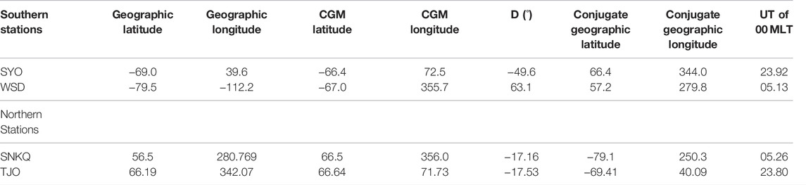
TABLE 1. Station location information for the southern and northern ground magnetometer data. From left to right the columns are station name, geographic latitude and longitude, corrected geomagnetic latitude and longitude, magnetic declination, and conjugate geographic latitude and longitude.

ACE IMF data from the magnetic field instrument (MFI) (Smith et al., 1998) and solar wind plasma data from the Solar Wind Electron, Proton, and Alpha Monitor (SWEPAM) (McComas et al., 1998) have been propagated from their original position near the L1 point to just in front of the nose of the magnetosphere at X = 17 R_E (Weygand and McPherron, 2006a; b). This was done by using Weimer mapping technique (Weimer et al., 2003, 2004) that uses a variation of the minimum variance method to estimate the orientation of IMF structures. These data are used to investigate correlations between the differences in onset times and the IMF and solar wind plasma properties.

Procedure and Observations

The first step is to identify onset events. For the first part of this study, we selected events with a sharp drop in the H component of the magnetic field in just the southern hemisphere stations, but not necessarily accompanied by any of the following: sharp drop in the H component in the opposite hemisphere, sharp drop in the AL index, auroral onset, auroral expansion phase, auroral recovery phase, magnetotail dipolarizations, or particle injections. This loose definition of onset could include PBIs, substorms, and pseudo breakups. All events were identified visually using the magnetometer data from either WSD/SNKQ or SYO/TJO. The criteria to qualify as an onset included 1) sharp drop in the H component over approximately 20 min period in both hemisphere, 2) H decrease ≥ 80 nT in both hemispheres, 3) event duration of more than 30 min, 4) the Z component in the northern and southern hemisphere to have approximately a 180° phase shift (as expected for a current wedge), 5) ≥ 3 h between onsets, and 6) the events should occur within 3 h of local midnight. Just under 1,000 onsets were identified using about 3.5 years of conjugate WSD/SNKQ and 12 years of SYO/TJO ground magnetometer data.

We understand there are a number of automated systems for selecting onsets, specifically substorm onsets, but none of these methods obtain the same results when compared with one another. Therefore, we have selected our events by-eye because it is the difference in the onset time between the opposite hemispheres that is the focus of this study, not the specific identification of substorms.

Figure 1 and Figure 2 show two examples of onsets that are observed at both WSD (blue curve, southern hemisphere) and SNKQ (black curve, northern hemisphere). The top panel shows the H component of the magnetic field, and the bottom panel shows the Z component. The black vertical line marks the visually selected onset time in the southern hemisphere, and the blue vertical line marks the visually selected onset time in the northern hemisphere, which will be discussed in the second part of this study. The cross correlation value for the H component and the difference in onset time determined from the cross covariance are shown in the bottom left portion of the top panel, while the bottom panel notes the cross correlation value for the Z component. Figure 1 shows an onset that occurred on 28 July 2010 at 0612:50 UT, and there was zero onset time difference between the two hemispheres. Figure 2 shows an onset that occurred in the southern hemisphere at 0643:20 UT on 22 February 2008 and ∼2.5 min after the onset in the northern hemisphere.

FIGURE 1

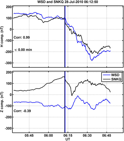
FIGURE 1. Example of onsets that simultaneously occur in both WSD (blue curve) in the southern hemisphere and the SNKQ (black curve) in the northern hemisphere. In the top panel is the H component of the magnetic field data and cross correlation coefficient and the onset time difference determined from cross covariance. The southern hemisphere onset is marked with the blue vertical line, and the northern hemisphere onset is marked with the black vertical line. In the bottom panel is the Z components and the cross correlation value.

FIGURE 2

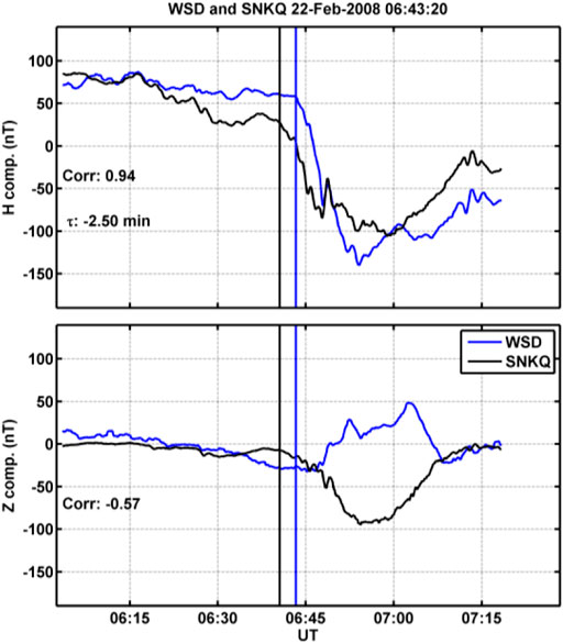
FIGURE 2. Example of onsets that occur at different times in the southern and northern hemispheres. This figure has the same format as Figure 1. In the top panel, the sharp drop in the H component of the magnetic field begins at SNKQ about 2.5 min before the WSD station.

While onset times were identified visually only in the southern hemisphere for the first part of this study, we performed a standard cross covariance between the north and south station of the pair to determine the lag time, for which there was a maximum correlation between the northern and southern time series. The cross covariance curve for the H component of the magnetometer data was determined using a data window extending 40 min before the onset and 35 min after the onset. We will explain below how this window was derived using a southern auroral electrojet index. This method provides an unbiased, clear, quantitative, and reproducible means for determining differences in onset time. The only potential weakness of this method is if the two onsets have significantly different slopes in their shape and different magnitudes of the change in the H component, then the cross correlation can underestimate the difference in onset time. This difference in the onset slope occurs in about 27% of the events.

We determined the size of the data window we used in each cross covariance of the H components of the magnetic field data by performing a superposed epoch of the cross covariance curves from over 440 onset events identified in the lower envelope of the southern auroral electrojet (SAL) index and the lower northern auroral electrojet (NAL) index developed by Weygand et al., (2008, 2014). The SAL index was developed using the same method as the standard world data center AL index from eight ground magnetometers in the auroral region in the southern hemisphere, and the NAL index is a near conjugate version of the SAL index. See Weygand et al., (2008, 2014) for more details. The SAL and NAL indices are used in the superposed epoch because they are, for the most part, an independent data set from the individual pairs of conjugate ground magnetometers. The AL index cross covariance curves were derived using 5 h of SAL and NAL index data on either side of an SAL onset time. The SAL onset time was identified visually using the criteria in Hsu and McPherron (2012), and that selection criteria included 1) sharp drop in the lower southern auroral electrojet (SAL) index over about 20 min period, 2) drop ≥100 nT, 3) ≥ 3 h between onsets, and 4) the SAL index accompanied by a decrease in the northern hemisphere NAL index.

Figure 3 shows the superposed epoch of the SAL/NAL cross covariance curves from 440 onset events. The time along the x-axis is the time lags from the cross covariance routine, and the y-axis is the cross correlation values. Epoch time zero is defined as the SAL index onset time. In Figure 3 we have defined the range of time to include in the cross covariance of the H components of the magnetic field (35–40 min) as the full width half max of the superposed epoch of the SAL/NAL cross covariance curves. See the horizontal red dash–dot curve in Figure 3. This range of time of 35–40 min is then used for the cross covariance of the onsets observed in the H component of the pairs of hemispheric conjugate magnetometer stations.

FIGURE 3

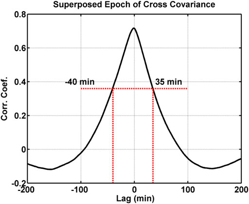
FIGURE 3. Superposed epoch of cross covariance curves for SAL and NAL indices for over 440 onsets identified in the SAL index. Epoch time zero is the onset time in the SAL index and the red horizontal dashed line is the full width half max of the peak of the cross correlation curve.

Figure 4 is a histogram of differences in onset time between the northern and southern hemisphere determined from the cross covariance of the H component of the conjugate pairs of ground magnetometers. Along the x-axis is the difference in onset time and the bin size is 1 min, and the histogram peaks off the y-axis scale at 753. Furthermore, the difference in onset time of the 0 s bin means the absolute value of the difference is less than 0.5 min. We have limited the y-axis range to 150 to better display the wings of the distribution, which are the important features of the distribution in this study. We note here that the temporal resolution of the SNKQ magnetometer data was decimated to 10 s in order to obtain differences in the onset time from cross covariance technique. The temporal resolution of the data used for the SYO-TJO pair was 1 s. The mean, standard deviation, and error of the mean are given in the upper right corner. The histogram consists of 976 events, and we have excluded events outside of three sigma and events with a cross correlation coefficient of the northern and southern H components of less than 0.6. Of the 976 event in the histogram, 518 (53%) have a difference in onset time of zero, and the other 47% have a non-zero different in onset time. In this figure, negative values indicate that the onset occurs earlier in the northern hemisphere, and positive values indicate the onset occurs earlier in the southern hemisphere. This is a significant result indicated that approximately half of the onsets exhibit interhemispheric timing differences. In our analysis, we attempted to unravel the causes for these differences.

FIGURE 4

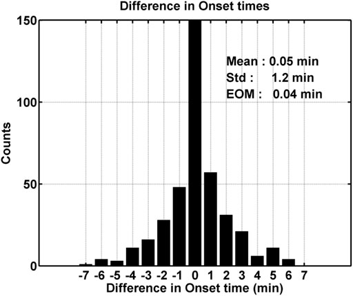
FIGURE 4. Histogram of differences in the onset time in the H component. The peak of the histogram at zero is off the y-axis scale and is at ∼800.

With all 976 hemispheric conjugate onsets, we examined any correlation that could occur between the differences in onset time and the IMF, solar wind plasma, season, UT, dipole tilt, and difference in the magnetic field line length. When we include all the hemispheric conjugate onsets, we found no strong correlation between the difference in onset time and IMF (including clock angle), solar wind speed, dynamic pressure that varied from 0.4 to 6.4 nPa, season, dipole tilt, and UT. Our results are described later in order. Figure 5 shows the difference in onset time with respect to the IMF By component using all the onsets including those with zero difference in offset time. The IMF By values are 1 h averages of the IMF taken from 68 min before the onset time to 8 min before the onset time. The 8 min delay is added to account for the time the solar wind propagates from the nose of the magnetosphere about 17 Re up stream to the approximate location of reconnection point in the magnetotail. The gray points are the individual events, the black points are means of the differences in onset time for IMF By bins 2 nT wide, and the mauve points are medians of the differences in onset time for IMF By bins 2 nT wide. The black error bars are the error of the mean, and the mauve error bars are the error of the median. We noted that 35 of the individual events are outside of the range of the y-axis. A shorter y-axis has been selected to better show the means of Δτ near 0 s. There is a small but statistically significant difference in the means of ∼+12 s for IMF By for the By bins at −2 and 0 nT. There is also the opposite time difference in the means of ∼ −12 s for IMF By in the + 4 nT bin. We see that negative time differences, that is, onset occurring first in the Northern Hemisphere, occur for positive or duskward IMF By. The median values, on the other hand, show no statistical difference from zero.

FIGURE 5

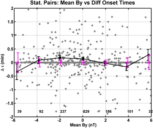
FIGURE 5. Differences in onset time versus IMF By. The gray points are the individual events, the black points are means of bins 2 nT wide, and the mauve points are medians of bins 2 nT wide. The error bars are the error of the mean and median. The values at the base of the figure indicate the number points per bin.

Figure 6 shows the same time difference with respect to IMF By as in Figure 5, except only the events that had a measurable, non-zero onset difference in time between the hemispheres are included. A comparison of Figures 5, 6 demonstrated that systematic trends are not immediately discernible for differences in onset times. However, the calculation of binned means reveal clear trends. When we subset our data in Figure 6 to only include differences in onset time within three standard deviations, cross correlation greater than 0.6, and include no 0 s differences in onset time, we found significant systematic trends in the differences in onset time as a function of the IMF By and season. In Figure 6, the differences in onset time in the IMF By mean bins at −2 and 0 nT have grown to about 24 s, and the difference in onset time is now about −24 s for the IMF By mean bin at + 4 nT. We believe the differences in onset time between 2 and 0 nT are due to twisting of the Earth’s magnetic field lines by IMF By that reduces the conjugacy between the station pairs. We will discuss this topic in more detail in the next section. However, the medians show no statistical difference from zero.

FIGURE 6

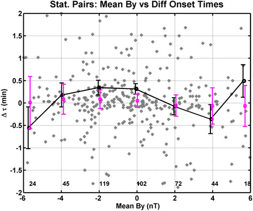
FIGURE 6. Format of this figure is the same as Figure 5, except for this figure we have excluded differences in onset time equal to 0 s.

Another systematic trend is also present when we plot the differences in onset times versus the difference in field line length. The assumption is that reconnection in the plasma sheet in the magnetotail is start of the onset whether it is a PBI, substorm, or pseudo break up. Differences in onset time could be associated with differences in the arrival of Alfvén waves produced at the reconnection point, which potentially have to traverse different distances due to warping of the tail field lines associated with dipole tilt or some other mechanism. To determine the difference in field line length, the magnetic field was mapped using the T96 model from the location of both magnetometers to the central plasma sheet, where the magnetic field changes direction in the Bx component. Figure 7 shows the difference in onset time as a function of the difference in the field line length between the southern and northern stations. The gray points in the figure are the individual events. We have widened the y-axis to better display the trend in the data. The black squares are means of the differences in onset time for bins 2 Re wide and the error bars are the error of the mean, and the mauve squares are medians of the differences in onset time for bins 2 Re wide and the error bars are the error of the mean and error of the median, respectively. Below each black square is the number of points in the bin. We have defined this trend as a very weak trend because the differences in onset time are only visible at the extreme differences in field line length where a small fraction of the data set is available (9 of 404 events use for the plot or ∼2% of the data). We also note that the extreme differences in field line length (−3.5, 3.9, and 5.5 Re) cannot be clearly associated with a specific range of dipole tilt, season, or IMF By values. That is to say, the individual events are distributed throughout the different seasons. Nearly all median values show no statistical difference from zero except for the value at about −3.5 Re.

FIGURE 7

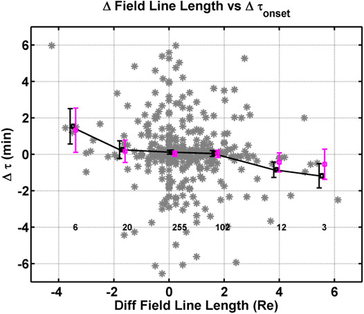
FIGURE 7. Differences in onset time versus as a function of the difference in the magnetic field line length (from the station to the central plasma sheet). The gray points are the individual events, the black points are means of bins 2 Re wide, and the mauve points are medians of bins 2 Re wide. The error bars are the error of the mean. The values at the base of the figure indicate the number points per bin.

The only other systematic change in the differences in onset time we found are seasonal. Figure 8 displays the difference in onset time as a function of the season (day of year). The gray points in the figure are the individual events. In addition, 10 points are off the scale, and we have shorted the y-axis to better display the trend in the data. The black squares are means of the difference in the onset time of bins 90 days wide centered on the black square, and the error bars are the error of the mean. The mauve squares are medians of the difference in the onset time of bins 90 days wide centered on the mauve square, and the error bars are the error of the median. Below each black square is the number of points in the bin. The blue vertical lines mark the spring equinox, summer solstice, autumnal equinox, and the winter solstice. The red curve is least squares fit of a sine wave to the median binned data points. The amplitude of the fit is 23.2 ± 4.4 s, the period of the sine wave is fixed to 365 days, and the phase is 65.5 ± 11.1 days. We remind the reader that the spring equinox occurs on the 79th day of the year. For Figure 8, we have only used IMF By values between 0.5 and 2.5 nT to limit the amount of twisting of the Earth’s magnetic field lines by IMF By. Finally, the extreme values from Figure 7 for differences in the field line lengths greater than 5.5 Re and less than −3.5 Re have not been included within Figure 8.

FIGURE 8

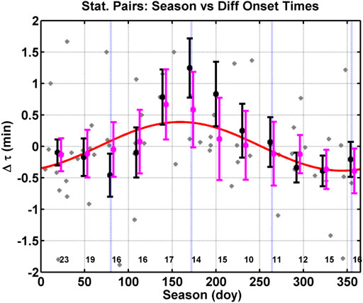
FIGURE 8. Difference in onset time versus season (day of year). The gray points are the individual events, the black squares are means of bins 90 days wide, and the mauve squares are medians of bins 90 days wide. The number of points per bin is given at the base of the plot. The error bars are errors of the mean and medians. The blue vertical lines mark the equinoxes and the solstices. The red curve is a sine wave fit to the black squares.

Figure 9 shows two examples of differences in the onset time for one summer solstice event on 17 July 201 at 0007:59 UT (left side) and one winter solstice event on 11 December 2003 at 2230:47 UT (right side). These plots both use the SYO-TJO pair of hemispheric conjugate stations and have approximately the same format as Figure 2. The red dashed line marks the onset time in the southern hemisphere. The purpose of these events is to show that the differences in onset time switches between summer and winter for individual events and is not just a statistical result in Figure 8. In the left side, the difference in the onset time is 0.5 min and the correlation coefficient is 0.96. The top left panel shows that the H component of SYO (blue) decreases before the H component of TJO (black). In the right side, the difference in onset time is −1.78 min and the correlation coefficient is 0.87. In this event the H component of TJO decreases before the H component of SYO.

FIGURE 9

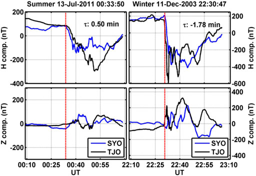
FIGURE 9. Format of this figure is approximately the same as Figure 2. The left side shows a summer solstice event and the right side shows a winter solstice event. The blue curve is associated with SYO, and the black curve shows the data from TJO. The red dashed line shows the onset time at SYO.

Discussion and Conclusion

In total, we have 976 hemispheric conjugate onsets with correlations above 0.6 and onsets in both hemispheres to investigate correlations with the IMF, solar wind plasma, and season. When we included all 976 events in our statistics, we found little to no correlation with the IMF, solar wind plasma, dipole tilt, UT, and season. However, when we subset the data to exclude differences in onset time equal to zero, then we saw a weak systematic variation associated with the IMF By, weak correlation with the difference in field line lengths, and a correlation with season. Here, we justify subsetting our data to exclude differences in onset time equal to zero. The correlation between the differences in onset time and season suggests that the ionospheric conductivity due to solar flux is responsible for the annual variation. There are a number of studies that have developed methods to determine the conductivity due to solar irradiation. Two of the more popular studies are Robinson and Vondrak (1984), which is an empirical model, and the other is the one used in the assimilative mapping of ionospheric electrodynamics (AMIE) procedure, which was develop developed by Richmond and Kamide (1988). These two studies indicate that the ionospheric conductivity for the stations with geographic latitudes similar to SYO and TJO would have a range of conductivity between 0.8 and 17 S for solar zenith angles between about 50° and 90° and f10.7 cm fluxes between 50 and 200 s. f.u. The average daily conductivity value varies systematically with season in both models such that the conductivity will be low in the midnight sector in the winter season and higher in the midnight sector in the summer season. However, it is well known that in addition to solar irradiance, particle precipitation from electron and ions determine the ionospheric conductivity. It has been shown for studies using electron precipitation from spacecraft measurements that during quiet and moderate geomagnetic conditions that the height integrated Hall conductivity, which would be most relevant to the onsets in the H component of the magnetic field, ranges between 0.5 and 17 S in the midnight sector (Vickrey et al., 1981; Hardy et al., 1987; Fuller-Rowel and Evans, 1987; McGranaghan et al., 2015). Moreover, during more active conditions, including substorm conditions, the height integrated Hall conductivity can be greater than 26 S (Hardy et al., 1987; Gjerloev and Hoffman, 2000), and in the study of Semeter and Doe (2002), it can be greater than 100 S in the midnight sector. If we assume that the particle precipitation is roughly equal in both hemispheres, then during some onsets the ionospheric conductivity due to particle precipitation may dominate ionospheric conductivity due to solar irradiance. Thus, ionospheric conductivity due to particle precipitation could obscure the systematic pattern associated with the differences in onset time associated with season. We used this assumption to justify removing the differences in onset that are equal to zero, which includes 518 onsets (53%). Note that the mean world data center AE index value for these 518 onsets is about 441 nT, the median is about 392 nT, and the error of the mean is 13 nT and for the not zero onset differences ,the mean is about 500 nT, the median is ∼460 nT, and the error of the mean is 15 nT. This simplistic examination of the AE indices does not support our assumption. However, the only way to test our assumption would require particle precipitation at the two conjugate locations, and this test is not feasible at this time.

Figure 6 shows the weak systematic correlation between the differences in onset time and means of the IMF By. The differences in onset time in the median bins versus IMF By show that from −2 to 0 nT the differences in onset time are on the order of 24 s and from 0 to 4 nT the differences in onset time are on the order of 0 s. We believe the difference in the onset time from −4 to 0 nT is due to twisting of the magnetic field lines by the IMF in the magnetotail. We support this statement by determining the conjugate position of the SYO and WSD stations on 12 September 2010 (arbitrarily selected date) using the T01 magnetic field model (Tsyganenko, 2002a; 2002b) with the model inputs: IMF Bz = −1 nT, dynamic pressure of 2.1 nPa, a Dst = −10 nT, and a range of IMF By from −6 nT to +6 nT. Figure 10 shows the change in position of the SYO station foot point location plotted over a map of Iceland with seven different IMF By values for times between 20 UT and 3 UT (left panel) and the change in position of the WSD station location plotted over a map of Falherty Island in Hudson bay with seven different IMF By values between 2 and 8 UT (right panel). Included on each plot are the geographic coordinates (black dashed lines) and the magnetic coordinates (gray dashed lines) some of which have been labeled. The red curve is for IMF By = + 6 nT, the orange curve for By = + 4 nT, the gold curve for By = + 2 nT, the black curve for By = 0 nT, the blue curve for By = −2 nT, the green curve for By = −4 nT, and the mauve curve for By = −6 nT. Each curve shows the change in the foot point over the 3 h on either side of local midnight for each station pair. For IMF By = +2 nT the TJO station and SYO foot point are approximately at the same MLT and the largest differences in magnetic longitude are about 7° for By = −6 nT, which would equate to an approximate difference in onset time of about 28 s for a westward surge of 1 MLT/min. In the right panel of Figure 10, the SNKQ station and WSD foot point are approximately at the same MLT for IMF By = 0 nT, and the largest differences in magnetic longitude are about 8° for By = +6 nT, which would equate to an approximate difference in onset time of about −32 s for a westward surge of 1 MLT/min. The difference in the IMF By aligned for the SYO/TJO and WSD/SNKQ pair of stations explains why our allowed IMF By range extends from 0.5 to 2.5 nT. We do not include 0 nT because the WSD/SNKQ pair contributes few onsets to this study and we want to limit the range of IMF By as much as possible to eliminate contribution from westward surges. These alignments for certain IMF By values explains why the difference in onset time is approximately zero in the By range of 0–4 nT. For IMF By of −2 nT, the foot point of the SYO station is located further toward the dawn where the SYO station could potentially record a westward surge before the TJO station. A similar statement can be made for the WSD/SNKQ pair of stations. This shift to the east explains why the difference in onset time is positive in Figure 6. However, the mean difference in onset time reverses sign for IMF By = −6 and 6 nT. Why these two difference in onset time at IMF By = −6 and 6 nT do not appear to follow the same trend as the other points is not clear at this time and may be due to low counting statistics.

FIGURE 10

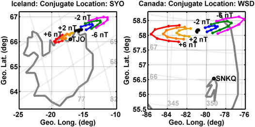
FIGURE 10. Map of Iceland and Hudson bay Canada showing the location of the TJO and SNKQ stations, which are indicated with the circle, and the change in the location of the SYO and WSD conjugate foot point with IMF By from −6 nT to +6 nT and dipole tilt for 3 h around local midnight.

Østgaard et al. (2004) also demonstrated the twisting of the magenotail field with IMF By with simultaneous substorm auroral onsets observed in opposite hemispheres. They showed in their study that the magnetic foot point of a magnetic field line in the southern hemisphere is duskward of the foot point in the northern hemisphere for IMF By < −2 nT and the foot point in the southern hemisphere is dawnward of the foot point in the northern hemisphere for IMF By > −1 nT. From this observations, we determined that for IMF By < −2 nT if an onset that occurs on a magnetic field line with its foot point directly over a southern hemisphere magnetometer station, then the northern magnetometer stations, which is conjugate to the southern station for IMF By = 0 nT, would record the onset later once the westward surge propagates to the northern station. More specifically, Østgaard et al. (2004) showed the difference in the MLT onset location shifted 0.13 MLT per 1 nT of IMF By. If we make three assumptions about our data set: 1) the onset in our study are substorm onsets, 2) the MLT difference between those onsets is about 0.26 MLT for 2 nT of IMF By, and 3) the typical westward surge for these substorms is about 1 MLT per minute (Angelopoulos et al., 2008a), then the difference in onset time with the twisting of the magnetic field is on the order of 16 s. The value of 16 s is consistent with the mean value of 24 ± 10 s in our Figure 6 at 2 nT.

If we now consider the medians, then no trend is apparent as a function of IMF By. This result does not agree with Østgaard et al. (2004). Even if we consider the results of Figure 8, which shows a seasonal dependence on the difference in onset time, and subset our data to the equinoxes, the median values still show no trend with IMF By. Ganushkina et al. (2013) showed a maximum displacement in the magnetic foot points on the order of 7° for an IMF By of |6| nT. For a westward surge moving with a speed of 1 MLT per min, this would amount to a potential difference in onset time of 30 s, which is smaller than the size of the error of the medians. The same can be said for smaller values of IMF By. With this data set, we cannot make definitive statements on the differences in onset time as a function of IMF By.

Figure 7 shows the difference in onset time as a function of the difference in the field line length between the southern and northern stations. The bulk of the medians are not statistically different from zero (only one data bin), and only half the means are statistically difference from zero. We questioned whether the values that are statistically different from zero have reasonable differences in onset time for the differences in field line length for typical plasma sheet Alfvén speeds. Using only the statistically significant points, we divided the difference in the field line length by the difference in onset time to determine the approximate Alfvén speed and obtained values ranging from 240 to 500 km/s. Typical plasma sheet Alfvén speeds are on the order of 300–1400 km/s (Lui, 1987; Angelopoulos et al., 2002; 2008b; Kan et al., 2011) depending on the location within the plasma sheet. These results suggest that the difference in onset time could be due to the differences in field line length; however, these results are only meaningful at the extremes and apply to only 21 events in those three difference bins of a total of 398 events used to produce the plot. Furthermore, we have made simplistic assumptions about Alfven travel times and used a magnetic field line model that is not ideal for activity periods within the magnetotail. We note that the relationship between magnetotail reconnection and onsets within the ionosphere is complicated and future studies should be performed to more rigorously investigate these findings.

In this study, we used cross covariance in order to determine the difference in onset time between the southern and northern magnetometer data. This method was used in order to minimize potential bias and provide a clear reproducible technique. However, as a means of further validating our results, we went through our onset events a second time and identified the possible onset time by-eye in the northern hemisphere data along with the southern hemisphere observations. See the black vertical lines in Figures 1, 2. Figure 11 displays the difference in onset time determined from the cross covariance method (x-axis) versus the difference in onset time determined from the by-eye method (y-axis). The gray points are individual events, and the black line is a linear fit to the data. The fit to the data is given in the upper left corner. The slope to the fit 1.15 ± 0.11 and the intercept is 0.31 ± 0.11 min. The slope indicates that the by-eye method for the northern hemisphere appears to result in a higher difference in onset time, but in general the results are similar.

FIGURE 11

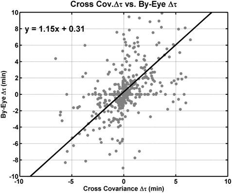
FIGURE 11. Difference in onset time determined from the cross covariance method versus the difference in onset time determined from the by-eye method. The gray points are individual events, and the black line is a linear fit to the data. The fit to the data is given in the upper left corner.

Our attempt to validate Figures 6–8 using the by-eye method to determine the difference in onset time produced several results. First, the trend observed in the difference in onset time versus magnetic field line length (i.e., our reexamination of Figure 7) is no longer present in both the means and the medians. Figure of the difference in onset time versus magnetic field line length redone using the northern hemisphere by-eye method data is not included in this study. Second, the trend in the difference in onset time versus IMF By is more apparent. See Figure 12, which has the same format as Figure 6. In Figure 12, the difference in onset time is now the difference between the onset in the southern and northern onsets that were selected by-eye. In general, the trend in both the means (black squares) and medians (mauve squares) is same within the uncertainties, and all the values are statistically different from zero. The difference in onset time between −4 and 0 nT is ∼21 s, with uncertainties around ±16 s in the median value. Furthermore, the difference in onset time become negative (about −26 s), with uncertainties on the order of ±19 s for IMF By values of 2 and 4 nT. These values are consistent with estimates, using the Ganushkina et al. (2013) results and westward surge propagation speed of 1 MLT/min.

FIGURE 12

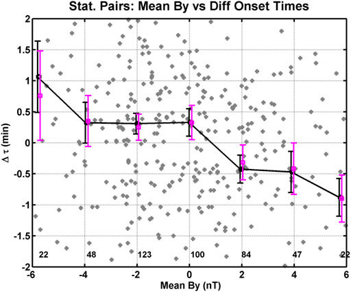
FIGURE 12. Format of this figure is the same as Figure 6, except for this figure we have used the southern and northern hemisphere onsets identified by-eye to determine the difference in onset time and excluded differences in onset time equal to 0 s.

Finally, the difference in onset time (using the results of the by-eye method) as a function of season is still present in the means even with the larger errors of the mean, but not as clear in the medians. Only the summer solstice value and the value at day of year 23 are statistically different from zero in the median because the errors on the medians have increased. See Figure 13, which has the same format as Figure 8. To be consistent with Figure 8 we have again limited the IMF By to a range of 0.5–2.5 nT. The amplitude of the sinusoidal fit to the median values is 28.8 ± 8.5 s, the period of the sine wave is fixed to 365 days, and the phase is 70.5 ± 16.9. Thus, we have obtained roughly the same results using the by-eye method for the difference in onset time as a function of season, but not for the difference in onset time as a function of IMF By and the difference in field line length.

FIGURE 13

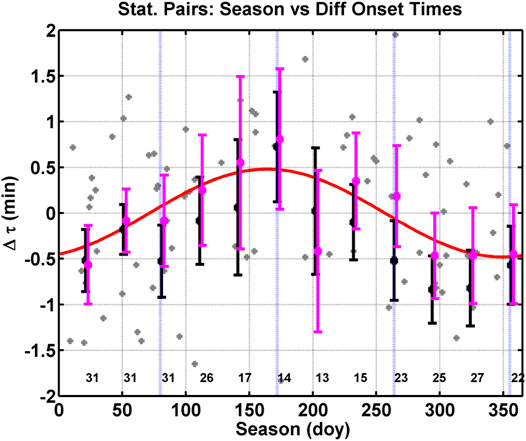
FIGURE 13. Format of this figure is the same as Figure 8. In this figure, we have used the southern and northern hemisphere onsets identified by eye to determine the difference in onset time.

In order to produce the results in many of the figures (i.e., Figures 5–8, 11 and Figure 12), we removed the differences in onset time equal to zero. However, there is information in these events. If the differences in onset time were due to IMF or solar wind plasma, then the number of onsets with differences in onset time equal to zero should be evenly distributed throughout the year and should have no seasonal dependence. Figure 14 is the fraction of onset times equal to zero per day of year bin as a function season for bins 90 days wide (i.e., the same size as for Figures 8, 13). To be consistent with Figure 8, we have limited the IMF By to a range of 0.5–2.5 nT. The vertical dashed lines mark the equinoxes and solstices. The figure displays peaks at the equinoxes and minima at the solstices validating our conclusion with this semi-independent method that the differences in onset time are a function of season.

FIGURE 14

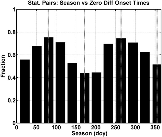
FIGURE 14. Fraction per bin of differences in onset time with a value of zero as a function of season (doy). The black bars are counts in bins 90 days wide, and the dotted vertical lines mark the equinoxes and the solstices.

In Figures 8, 13, 14, we limited the IMF By affects by limiting the range of IMF By to 0.5–2.5 nT. This range was selected to include enough events for good statistics. With the remaining onsets, we showed, in Figure 8, that the difference in onset time is dependent on the season or more likely annual variation of ionospheric conductivity due to sunlight. In Figure 15, we demonstrated the annual variation in ionospheric conductivity and plotted the solar radio flux (S) f10.7 cm in the top panel, the solar zenith angle (SZA) for both TJO (blue) and SYO (red) in the second panel, and the TJO (third panel) and SYO (fourth panel) height integrated conductivity ∑ = 1.5 (S cos (SZA))^0.5 derived in Robinson and Vondrak (1984). The first panel shows the radio flux varies between 50 and 200 s.f.u. The second panel shows the SZA varies between about 50° and 140°, and for values above 90° (marked with the dashed line) the station is in the nightside and receives no sunlight. Note that the scattering on the TJO station is larger than that on the SYO station because TJO is at a lower geographic latitude and experiences a larger range of solar zenith angles. In the third panel, the height integral solar ionospheric conductivity is largest for TJO in the northern summer season, and in the fourth panel, the conductivity for SYO is largest in the southern summer season. We noted that the height integrated conductivity is set to 1 S in Robinson and Vondrak (1984) when the ionosphere is not sunlit. The second, third, and fourth panels of Figure 15 demonstrate the seasonal change in ionospheric conductivity due to solar illumination.

FIGURE 15

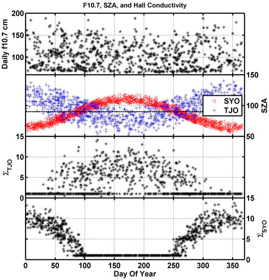
FIGURE 15. Variation of height-integrated ionospheric conductivity due to solar illumination as a function of the day of year for all our onset events. In the top panel is the solar radio flux at 10.7 cm, and in the second panel is the solar zenith angle for TJO (blue) and SYO (red). The dashed line marked a SZA = 90°. The third panel show the TJO height-integrated ionospheric conductivity, and the forth panel show the conductivity for SYO.

The sinusoidal variation in the differences in onset time has a significant impact on substorm models. Figure 8 shows that onsets occur first in the unlit midnight sector by about 23 s before the sunlit hemisphere during the summer and winter solstices. To explain this difference in onset time, we can think of the ionosphere as an inductor resistor (LR) series circuit. In LR circuit the growth time of the current is τ = L/R or τ = L∑, where ∑ is the conductance. If we assume that the inductance is the same in both hemispheres, then when the conductance is large, as in the sunlit ionosphere, the growth time of the ionospheric current is long and when the conductance is small, like in the unlit ionosphere, the growth time is small. Substorm onset models do not take the differences in ionospheric conductivity into account at this time; a difference of 23 s between the two hemispheres may influence the identification of an ideal substorm model. Recall that the difference between the start of the tail reconnection and the auroral onset in the outside-in model is about 120 s, where a 23 s difference in the auroral onset is about 19%. The difference between the start of current disruption and the auroral onset is 30 s for the inside-out, where a 23 s difference in the auroral onset is about 76%. Hence, our results cannot distinguish between the outside-in or inside-out models. However, we believe it is important for substorm models and future substorm studies to take into account the state of the ionosphere. Fortunately, most substorm studies identify auroral onsets with all sky images in the unlit hemisphere because they are limited to visible wavelengths; however, ultraviolet imagers onboard spacecraft are not restricted to unlit conditions. Future ultraviolet imagers with a cadence better than 23 s should be able to observe this difference in onset time as a function of season.

Data Availability Statement

The raw data supporting the conclusions of this article will be made available by the authors, without undue reservation.

Author Contributions

AK provided ground magnetometer data from Antarctica and Iceland. EZ provided ground magnetometer data from Antarctica, funding, data analysis, data interpretation, guidance, and helped with editing this manuscript. DMO provided funding and helped with editing this manuscript. JMW wrote the manuscript, performed the data analysis, performed the data interpretation, produced the figures, and helped with editing this manuscript.

Funding

This study was made possible by NASA THEMIS contract NAS5-02099 at UCLA; NSF Antarctic Aeronomy and Astrophysics, Office of Polar Programs grant ANT-1043621; and NSF Directorate of Atmospheric and Geosciences grant 1606014, and NASA HGI grant 80NSSC22K0756.

Conflict of Interest

The authors declare that the research was conducted in the absence of any commercial or financial relationships that could be construed as a potential conflict of interest.

Publisher’s Note

All claims expressed in this article are solely those of the authors and do not necessarily represent those of their affiliated organizations, or those of the publisher, the editors, and the reviewers. Any product that may be evaluated in this article, or claim that may be made by its manufacturer, is not guaranteed or endorsed by the publisher.

Acknowledgments

We thank the many different groups operating magnetometer arrays for providing data for this study including: The Canadian Magnetic Observatory Network (CANMON) for data from SNKQ is maintained and operated by the Geological Survey of Canada—http://gsc.nrcan.gc.ca/geomag and National Institute of Polar Research in Japan for data from the TJO and SYO stations. We thank the CSA for logistical support in fielding and data retrieval from the GBO stations. The authors thank E. Yizengaw, M. B. Moldwin, and the rest of the SAMBA team for the WSD magnetometer data. SAMBA was also operated by UCLA and funded by NSF. We would also like to thank M.G. Kivelson, K.K. Khurana, R.L. McPherron, R.J. Strangeway, V. Angelopoulos, and R.J. Walker for their invaluable input. We acknowledge the IUGONET system for providing the data from Tjornes and Syowa Station and contribution of Dr. Yoshimasa Tanaka who is the leader of the IUGONET development team.

References

Angelopoulos, V., Chapman, J. A., Mozer, F. S., Scudder, J. D., Russell, C. T., Tsuruda, K., et al. (2002). Plasma Sheet Electromagnetic Power Generation and its Dissipation along Auroral Field Lines. J. Geophys. Res. Space Phys. 107 (A8). doi:10.1029/2001ja900136

CrossRef Full Text | Google Scholar

Angelopoulos, V., McFadden, J. P., Larson, D., Carlson, C. W., Mende, S. B., Frey, H., et al. (2008b). Tail Reconnection Triggering Substorm Onset. Science 321 (5891), 931–935. doi:10.1126/science.1160495

PubMed Abstract | CrossRef Full Text | Google Scholar

Angelopoulos, V., Sibeck, D., Carlson, C. W., McFadden, J. P., Larson, D., Lin, R. P., et al. (2008a). First Results from the THEMIS Mission. Space Sci. Rev. 141, 453–476. doi:10.1007/s11214-008-9378-4

CrossRef Full Text | Google Scholar

Baker, D. N., Pulkkinen, T. I., Angelopoulos, V., Baumjohann, W., and McPherron, R. L. (1996). Neutral Line Model of Substorms: Past Results and Present View. J. Geophys. Res. 101 (A6), 12975–13010. doi:10.1029/95JA03753

CrossRef Full Text | Google Scholar

Baumjohann, W., Paschmann, G., and Cattell, C. A. (1989). Average Plasma Properties in the Central Plasma Sheet. J. Geophys. Res. 94, 6597–6606. doi:10.1029/ja094ia06p06597

CrossRef Full Text | Google Scholar

Boudouridis, A., and Zesta, E. (2007). Comparison of Fourier and Wavelet Techniques in the Determination of Geomagnetic Field Line Resonances. J. Geophys. Res. 112, a–n. doi:10.1029/2006JA011922

CrossRef Full Text | Google Scholar

Frank, L. A., and Sigwarth, J. B. (2003). Simultaneous Images of the Northern and Southern Auroras from the Polar Spacecraft: An Auroral Substorm. J. Geophys. Res. 108 (A4), 8015. doi:10.1029/2002JA009356

CrossRef Full Text | Google Scholar

Fuller-Rowell, T. J., and Evans, D. S. (1987). Height-integrated Pedersen and Hall Conductivity Patterns Inferred from the TIROS-NOAA Satellite Data. J. Geophys. Res. 92, 7606–7618. doi:10.1029/ja092ia07p07606

CrossRef Full Text | Google Scholar

Ganushkina, N. Y., Kubyshkina, M. V., Partamies, N., and Tanskanen, E. (2013). Interhemispheric Magnetic Conjugacy. J. Geophys. Res. Space Phys. 118, 1049–1061. doi:10.1002/jgra.50137

CrossRef Full Text | Google Scholar

Gjerløv, J. W., and Hoffman, R. A. (2000). Height‐integrated Conductivity in Auroral Substorms: 1. Data. J. Geophys. Res. Space Phys. 105 (A1), 215–226.

Google Scholar

Hardy, D. A., Gussenhoven, M. S., Raistrick, R., and McNeil, W. J. (1987). Statistical and Functional Representations of the Pattern of Auroral Energy Flux, Number Flux, and Conductivity. J. Geophys. Res. 92 (A11), 12275–12294. doi:10.1029/ja092ia11p12275

CrossRef Full Text | Google Scholar

Hones, E. W. (1976), “The Magnetotail: its Generation and Dissipation,” in Physics of Solar Planetary Environments, Editor D. J. Williams, (Washington, D.C., USA: AGU), Vol. 558.

Google Scholar

Hsu, T.-S., and McPherron, R. L. (2012). A Statistical Analysis of Substorm Associated Tail Activity. Adv. Space Res. 50 (10), 1317–1343. doi:10.1016/j.asr.2012.06.034

CrossRef Full Text | Google Scholar

Kan, J. R., Li, H., Wang, C., Frey, H. U., Kubyshkina, M. V., Runov, A., et al. (2011). Brightening of Onset Arc Precedes the Dipolarization Onset: THEMIS Observations of Two Events on 1 March 2008. Ann. Geophys. 29 (11), 2045–2059.

CrossRef Full Text | Google Scholar

Kivelson, M. G., Khurana, K. K., Walker, R. J., Kepko, L., and Xu, D. (1996). Flux Ropes, Interhemispheric Conjugacy, and Magnetospheric Current Closure. J. Geophys. Res. 101 (27), 341350. doi:10.1029/96ja02220

CrossRef Full Text | Google Scholar

Lui, A. T. (1987). Magnetotail Physics. Baltimore, MD: Johns Hopkins University Press.

Google Scholar

Lui, A. T. Y. (1996). Current Disruption in the Earth's Magnetosphere: Observations and Models. J. Geophys. Res. 101, 13067–13088. doi:10.1029/96ja00079

CrossRef Full Text | Google Scholar

Lui, A. T. Y., Lopez, R. E., Krimigis, S. M., McEntire, R. W., Zanetti, L. J., and Potemra, T. A. (1988). A Case Study of Magnetotail Current Sheet Disruption and Diversion. Geophys. Res. Lett. 15, 721–724. doi:10.1029/gl015i007p00721

CrossRef Full Text | Google Scholar

McComas, D. J., Bame, S. J., Barker, P., Feldman, W. C., Phillips, J. L., Riley, P., et al. (1998). Solar Wind Electron Proton Alpha Monitor (SWEPAM) for the Advanced Composition Explorer. Space Sci. Rev. 86, 563–612. doi:10.1007/978-94-011-4762-0_20

CrossRef Full Text | Google Scholar

McGranaghan, R., Knipp, D. J., Matsuo, T., Godinez, H., Redmon, R. J., Solomon, S. C., et al. (2015). Modes of High‐latitude Auroral Conductance Variability Derived from DMSP Energetic Electron Precipitation Observations: Empirical Orthogonal Function Analysis. J. Geophys. Res. Space Phys. 120, 11,013–11,031. doi:10.1002/2015JA021828

CrossRef Full Text | Google Scholar

Morioka, A., Miyoshi, Y., Tsuchiya, F., Misawa, H., Kasaba, Y., Asozu, T., et al. (2011). On the Simultaneity of Substorm Onset between Two Hemispheres. J. Geophys. Res. 116, a–n. doi:10.1029/2010JA016174

CrossRef Full Text | Google Scholar

Newell, P. T., Sotirelis, T., and Wing, S. (2010). Seasonal Variations in Diffuse, Monoenergetic, and Broadband Aurora. J. Geophys. Res. 115, a–n. doi:10.1029/2009JA014805

CrossRef Full Text | Google Scholar

Ohtani, S., Wing, S., Ueno, G., and Higuchi, T. (2009). Dependence of Premidnight Field-Aligned Currents and Particle Precipitation on Solar Illumination. J. Geophys. Res. 114, a–n. doi:10.1029/2009JA014115

CrossRef Full Text | Google Scholar

Østgaard, N., Mende, S. B., Frey, H. U., Immel, T. J., Frank, L. A., Sigwarth, J. B., et al. (2004). Interplanetary Magnetic Field Control of the Location of Substorm Onset and Auroral Features in the Conjugate Hemispheres. J. Geophys. Res. 109, A07204. doi:10.1029/2003JA010370

CrossRef Full Text | Google Scholar

Østgaard, N., Mende, S. B., Frey, H. U., Sigwarth, J. B., Åsnes, A., and Weygand, J. M. (2007). Auroral Conjugacy Studies Based on Global Imaging. J. Atmos. Solar-Terrestrial Phys. 69, 249–255. doi:10.1016/j.jastp.2006.05.026

CrossRef Full Text | Google Scholar

Richmond, A. D., and Kamide, Y. (1988). Mapping Electrodynamic Features of the High-Latitude Ionosphere from Localized Observations: Technique. J. Geophys. Res. 93, 5741–5759. doi:10.1029/ja093ia06p05741

CrossRef Full Text | Google Scholar

Robinson, R. M., and Vondrak, R. R. (1984). Measurements ofEregion Ionization and Conductivity Produced by Solar Illumination at High Latitudes. J. Geophys. Res. 89 (A6), 3951–3956. doi:10.1029/JA089iA06p03951

CrossRef Full Text | Google Scholar

Sato, N., Nagaoka, T., Hashimoto, K., and Saemundsson, T. (1998). Conjugacy of Isolated Auroral Arcs and Nonconjugate Auroral Breakups. J. Geophys. Res. 103, 11641–11652. doi:10.1029/98JA00461

CrossRef Full Text | Google Scholar

Semeter, J., and Doe, R. (2002). On the Proper Interpretation of Ionospheric Conductance Estimated through Satellite Photometry. J. Geophys. Res. 107 (A8), 19. doi:10.1029/2001JA009101

CrossRef Full Text | Google Scholar

Smith, C. W., L’Heureux, J., Ness, N. F., Acuña, M. H., Burlaga, L. F., and Scheifele, J. (1998). The ACE Magnetic Fields Experiment. Space Sci. Rev. 86, 613–632. doi:10.1007/978-94-011-4762-0_21

CrossRef Full Text | Google Scholar

Tsyganenko, N. A. (2002a). A Model of the Near Magnetosphere with a Dawn-Dusk Asymmetry 1. Mathematical Structure. J. Geophys. Res. 107 (A8), 12. doi:10.1029/2001JA000219

CrossRef Full Text | Google Scholar

Tsyganenko, N. A. (2002b). A Model of the Near Magnetosphere with a Dawn-Dusk Asymmetry 2. Parameterization and Fitting to Observations. J. Geophys. Res. 107 (A7), 10–11. doi:10.1029/2001JA000220

CrossRef Full Text | Google Scholar

Vickrey, J. F., Vondrak, R. R., and Matthews, S. J. (1981). The Diurnal and Latitudinal Variation of Auroral Zone Ionospheric Conductivity. J. Geophys. Res. 86 (A1), 65–75. doi:10.1029/ja086ia01p00065

CrossRef Full Text | Google Scholar

Weimer, D. R. (2004). Correction to “Predicting Interplanetary Magnetic Field (IMF) Propagation Delay Times Using the Minimum Variance Technique. J. Geophys. Res. Space Phys. 109, A12. doi:10.1029/2004ja010691

CrossRef Full Text | Google Scholar

Weimer, D. R., Ober, D. M., Maynard, N. C., Collier, M. R., McComas, D. J., Ness, N. F., et al. (2003). Predicting Interplanetary Magnetic Field (IMF) Propagation Delay Times Using the Minimum Variance Technique. J. Geophys. Res. 108. doi:10.1029/2002JA009405

CrossRef Full Text | Google Scholar

Weygand, J. M., and McPherron, R. L. (2006b). ACE SWEPAM Solar Wind Weimer Propagated 60 S Resolution Data in GSM Coordinates. doi:10.21978/P8S62R

CrossRef Full Text | Google Scholar

Weygand, J. M., and McPherron, R. L. (2006a). ACE Weimer Propagated 60 S Resolution Tri-axial Fluxgate Magnetometer in GSM Coordinates. doi:10.21978/P8933R

CrossRef Full Text | Google Scholar

Weygand, J. M., and Zesta, E. (2008). Comparison of Auroral Electrojet Indices in the Northern and Southern Hemispheres. J. Geophys. Res. 113, a–n. doi:10.1029/2008JA013055

CrossRef Full Text | Google Scholar

Weygand, J. M., Zesta, E., and Troshichev, O. (2014). Auroral Electrojet Indices in the Northern and Southern Hemispheres: A Statistical Comparison. J. Geophys. Res. Space Phys. 119, 4819–4840. doi:10.1002/2013JA019377

CrossRef Full Text | Google Scholar