Making an executable paper with the Python in Heliophysics Community to foster open science and improve reproducibility

1 Introduction

We recount how we made this paper, the first executable paper in Heliophysics, to highlight the benefits of our process. Executable papers are a new kind of paper written in software that combines text, data, and code to enable readers to reproduce every step taken to arrive at the paper’s conclusions (Lasser 2020). Our executable paper is centered around an adaptable Python workflow to compare magnetosphere models to spacecraft observations. It is one example of many other workflows that can be developed through collaborations between software developers and scientists in a move towards open science. We detail how our process was facilitated by such a collaboration and guided by open science principles.

The following subsections provide the background to understand this work. We set the scene in Section 1.1 by discussing open science and how it relates to issues with reproducibility. Then we describe the organization from which our team originates, the Python in Heliophysics Community (PyHC), and how our goals align with this work in Section 1.2. Then we fully explain the concept of executable papers in Section 1.3—what they are, why they benefit reproducibility, and how they compare to traditional papers. Next, we discuss the cross-disciplinary collaboration underpinning our work and why it was crucial to our success in Section 1.4. Then we give the science background to follow the workflow presented in our executable paper before actually presenting it in Section 1.5. The following “Method” section contains the workflow (Section 2). We will showcase it fully, from the underlying concepts to the implementation using our PyHC packages. Section 3 covers the results and outcomes from our work. Finally, we end the paper with our closing remarks in Section 4.

1.1 Open science and reproducibility

Open science is a disruptive new approach to the scientific process based on cooperative work and new ways of diffusing knowledge by using digital technologies and new collaborative tools (FOSTER 2022). It is about extending the principles of openness to the whole research cycle, fostering sharing and collaboration as early as possible. These principles are at the heart of this work, but it may be intriguing to note that this is our interpretation of open science. It is a new enough concept that it does not yet have an exact formal definition. One systematic literature review came up with the concise definition: “Open science is transparent and accessible knowledge that is shared and developed through collaborative networks” (Vicente-Saez and Martinez-Fuentes 2018). However it is interpreted, we aim to make it a pivotal conversation within the field of Heliophysics. The increased ease of reproducing research gained from the sharing of raw data and research materials is a strong motivator for our work.

It has been six years since a Nature survey “lifted the lid on the reproducibility crisis” (Baker 2016) and scientific communities are still grappling with the issue. The frequency of crisis narratives in publications has skyrocketed (Fanelli 2018; Nelson et al., 2021), but progress has been hampered by a lack of technical computer skills needed to make the results and supporting work in publications reproducible (Bajpai et al., 2017; Cacho and Taghva 2020) along with disagreements on what “reproducibility” means (Baker 2016b). The severity of the crisis (or whether there is one at all) is still debated, but it spawned a growing push to bring reproducible, open science practices into the mainstream. A significant outcome of this push has been the NASA TOPS (Transform to OPen Science) initiative (Gentemann et al., 2021). This five-year initiative designates 2023 as the “Year of Open Science,” and it will accelerate the engagement of the scientific community in open science practices through coordinated events and activities.

PyHC embraces open science, and as members of PyHC, we support this push by encouraging the Heliophysics community to create executable papers. We describe how we developed our executable paper by coordinating efforts between scientists and software developers. The purpose of this work is to present our methodology as an example to the community of a more sustainable approach to reproducibility, particularly lessening the increasing demand on the scientists involved.

1.2 The Python in Heliophysics Community

PyHC is an international, multi-organizational community that serves as a knowledge base for performing Heliophysics research in the Python programming language (Ware and Roberts 2019). Our mission is to facilitate scientific discovery by promoting the use and development of sustainable open-source Python software across the solar and space physics community; to improve communication and collaboration between disciplines, developers, and users; to establish and maintain development standards (PyHC 2022d); and to foster interoperability and reproducibility.

Recent years have seen an incredible boom in both the amount of space science data and the software tools used to dissect and investigate it. The problem of today is not “does a tool exist to do this research,” but rather “how does one quickly find which tool is used to do this research?” PyHC was formed in 2018 to help answer this problem for the Heliophysics and space weather communities. PyHC has done the work of bringing together key members in these communities, organizing community activities, and identifying potential areas for collaboration and integration. This information is housed in a centralized location, the PyHC website (PyHC 2022c), which has over 60 Heliophysics Python packages (PyHC 2022a) and a gallery of examples (PyHC 2022b) about how to use them.

The idea behind this project came from a PyHC telecon during which we were brainstorming new examples for the PyHC Gallery. We wanted an example that showed multiple packages chained together in a unified workflow, which led us to the workflow we demonstrate in the “Method” section below. As we worked on this, however, we came to realize that others could benefit from learning how we conducted our work. So, the idea grew into this paper at hand. Comparing magnetosphere models to spacecraft observations is an interesting scientific use case, and in chaining together our packages we made a novel workflow that is easier than previous ones, but we are putting the spotlight on our process rather than the science. We could have easily written about any number of other use cases and still made the same point.

1.3 Executable papers

Traditional publications face a variety of issues in the context of reproducibility: missing raw or original data, lack of a tidied-up version of the data, no source code available, or lacking the software to run the experiment. Furthermore, even when all these tools are available, a lack of documentation or deprecated dependencies can make replicating the research a non-trivial task (Cacho and Taghva 2020). In contrast, executable papers include all components of the research. As such, developing one is a significant effort worthy of recognition independent of the typical publication. A current lack of recognition discourages significant effort in this area, however, as indicated by the publication history described in Dr. Jana Lasser’s article “Creating an executable paper is a journey through Open Science” (2020):

There was a short outburst of activity back in 2011, driven by Elsevier (Elsevier n.d.), but other than that little turns up when searching for the term online. Other than a couple of templates (Akhlaghi n.d.), very short guidelines (Reproducible Research n.d.), or very detailed but not very broadly applicable how-to’s (CodaLab 2020), there is currently not much to build on.

In that spirit, this work aims to provide a broadly applicable example of how to build an executable paper in Heliophysics—the first of its kind.

The idea of an executable paper is to enable readers to reproduce the steps taken to arrive at a publication’s conclusions, from the raw data to polished figures and everything in-between, and to build directly upon the work. It is an interactive document that puts the publication’s text inline with the code used in the research, in an environment with the data and dependencies needed to run the code. The environment holding these components is an internal container such as a Docker container (Docker 2022). This containerization means there is never a need to find and download data nor install any software. It also means the executable paper is isolated from any problems that may arise with future versions of the installed software packages, because the current package versions are preserved in working order inside the container.

Executable papers are a fairly new concept with little standardization, but have been gaining traction, particularly with Python-related research, due to the growing popularity of Jupyter notebooks (Jupyter 2022). At present, executable papers are Jupyter notebooks—for Python code, at least. It does not have to be this way; executable papers are a concept more abstract than Jupyter notebooks. There just does not yet exist an alternate implementation that satisfies the requirements. Because readers can copy a Jupyter notebook and modify it without changing (and potentially breaking) it for others, the executable paper format gives readers a better launching point than traditional papers to produce new research based on the same or similar processes. In contrast, when a paper’s methods are only described generically in prose, one might easily come up with different “false cognate” solutions that do not directly replicate the original work. This is especially true when multiple packages are used. Executable papers prevent this by unambiguously showing what code to run when—typically referred to as “direct replication” (American Society for Cell Biology 2015)—and by enabling users to directly build upon the work.

We encourage the Heliophysics community to make executable papers, although we recognize that most impactful journals do not yet accept executable papers as formal submissions. They therefore fulfill the role of an extended preprint that exists next to the publication in the journal (Lasser 2020). Most journals do not typically accept executable papers because there are unsolved problems with them. Chief among them is the maintenance and background support required to keep them working for long periods of time. For example, it is not unheard of to reference papers that are, say, 80–100 years old. It is hard to fathom that level of support being supplied to executable papers (or any software, for that matter) for such a long period of time. Containerization adds stability to executable papers, but only when 100% of all the research’s components are inside the container. If, for example, the data were stored on a separate server because it did not fit in the container, then that executable paper’s reproducibility would only be valid for as long as the linked data was available. Additionally, making executable papers takes extra work and a certain level of technical proficiency. We recognize the stability problem as well outside the scope of this paper. However, we address the technical proficiency problem by forming a collaboration between a collection of scientists and software developers, distributing the work according to their expertise. We pause here to briefly describe the notebook platform we chose for this project, Deepnote, because it uniquely facilitated this collaborative development.

1.3.1 Deepnote

Deepnote is a cloud-based notebook platform with all the standard Jupyter functionalities as well as real-time collaboration (Deepnote 2022). It is newer than its well-established competitors (which we discuss in “Supplementary Appendix B”) and, in fact, just came out of beta in May 2022. Despite its newness, Deepnote’s real-time collaborative editing capability swayed us into choosing it. Users of Google Docs will be familiar with this feature; everyone works on the same document simultaneously, and all edits are immediately reflected in real-time for everyone.

In addition to this feature, Deepnote supports everything necessary to make an executable paper. It offers fully-customizable environments for each notebook to handle software dependencies (through Docker images). It offers a persistent file system within these environments to store data, other media, and the notebooks themselves. It offers integrations with third-party large-file storage services to manage data files that exceed the default storage limits. It even has a feature to publish and host notebooks as publicly-available “articles”, which is particularly well-suited for sharing executable papers. We shared ours using that feature.¹ Although, in recognition that platforms can change and links can break, we also uploaded our Docker image files to Zenodo in order to obtain a DOI.²

1.4 Collaboration

Our team consists of scientists and PyHC members, most serving a software development role, some serving as topic experts to help with the science. Some have backgrounds in both roles but served in only one role for this project. This cross-disciplinary collaboration made us more capable. A single team member aiming to complete the entire task would have been faced with either a lack of scientific, software, or technical expertise, depending on the team member’s background, which typically makes such a project too time consuming. Our developers did not know enough about the science of magnetospheres and our scientists did not know enough about the software. But, in distributing work according to our expertise, we completed the task with relative ease. We hope this is encouragement for readers finding themselves daunted by a similar task.

We developed this executable paper together in a single shared Jupyter notebook. Deepnote’s real-time collaboration made this simple and convenient. Effort was taken from the beginning by everyone to document and explain the steps of their work as comments in the notebook, instead of separately elsewhere. This allowed us to understand each other’s work and made it so that much of the paper was already written by the time development ended. To give two examples of task distribution: Eric Grimes wrote the portions of this paper that use pySPEDAS because he leads development of the pySPEDAS project, and Yihua Zheng provided guidance about the magnetosphere models we used because she is one of our topic experts. We note that more scientists could easily be included in the group, and the number of software developers in the group could easily be fewer, all depending on the complexity of the science question being addressed and the software needed. See “Supplementary Appendix A” for descriptions of our team members, including their backgrounds and contributions to this project.

1.5 Comparing magnetosphere models to spacecraft observations

We present the current executable workflow as an example of the level of open science and reproducibility possible through this approach. We have covered our process for developing the workflow, so, let us finally turn to the science of its contents: comparing magnetosphere models to spacecraft observations. The magnetosphere is the region in which Earth’s magnetic field is the predominant effective magnetic field (NASA 2022). The magnetopause is the magnetosphere’s outer limit (Merriam-Webster 2022). In this simple workflow, we can detect where the magnetopause is by observing magnetopause crossings in spacecraft readings, test the accuracy of empirical magnetopause models by comparing the observed locations to modeled ones, and validate physics-based magnetosphere models by virtually flying spacecraft through them and comparing the modeled readings to the observed data. This is made possible by five PyHC packages: pySPEDAS, SpacePy, PlasmaPy, PyTplot, and Kamodo. We describe these packages in “Supplementary Appendix C.”

Empirical magnetopause models, such as the one created by Shue et al., estimate where the magnetopause is by deriving a functional form that depends on solar wind parameters. The Shue et al. function represents the shape of the magnetopause and its scale (represented by the standoff distance on the Sun-Earth line) depending on the solar wind parameters (Shue et al., 1998). Physics-based models, such as the Open Geospace General Circulation Model (OpenGGCM), model the magnetosphere by deriving its properties from physical first principles, and provide the global state of the entire geospace (which includes the magnetosphere) (Community Coordinated Modeling Center, 2022). We compare these modeled data to data from NASA’s Magnetospheric Multiscale Mission (MMS), which orbit Earth and regularly cross the magnetopause boundary.

We demonstrate how to use SpacePy functions to calculate metrics from MMS data to detect where these crossings happen and compare the calculated locations to those estimated by the Shue et al. model to test the model’s accuracy. MMS also takes other magnetosphere readings as it orbits, such as magnetic field components, which can be used to calculate plasma parameters. We show how to use PlasmaPy to calculate plasma parameters from these readings to augment our detections of magnetopause crossings. We also show how to virtually fly MMS through the OpenGGCM model and compare the modeled readings to the observed data using Kamodo’s flythrough capability, again to test the model’s accuracy. This workflow is depicted in Figure 1. Although we use MMS data with the Shue et al. and OpenGGCM models in this example, the workflow can be easily adapted to numerous datasets and models available through these and other packages.

FIGURE 1

FIGURE 1. A flowchart depicting our workflow to compare magnetosphere models to spacecraft observations.

1.5.1 Data specifics

We use science-quality level 2 fast survey data from MMS probe 1 that is preloaded into our container’s file system. Specifically, we use: MMS Ephemeris and Coordinates (MEC) data to retrieve the spacecraft’s location, Fluxgate Magnetometer (FGM) data to measure the magnetic field strength experienced by the spacecraft, and Ion moments from the Fast Plasma Investigation (FPI) data to show how the ion population changes as the spacecraft crosses the magnetopause. We look at data from 16 October 2015 because data from that date is used in several papers to compare observational data to model data (Burch et al., 2016; Alm et al., 2017; Egedal et al., 2017).

The OpenGGCM model data we use was generated by CCMC for this work and is also stored in our file system. Other model data outputs are freely available to the public by request (https://ccmc.gsfc.nasa.gov/). Our model (ID Yihua_Zheng_040122_1) uses default settings with OpenGGCM 5.0, Rice Convection Model (RCM) 1.0, and OMNI data (Qin et al., 2007) as solar wind input. Specific input parameters are given as a footnote.³ To save storage space, our model was intentionally generated at such a coarse resolution that it is not useful for deep scientific analysis.⁴

2 Methods

We turn to our workflow to compare magnetosphere models to spacecraft observations.

2.1 Imports

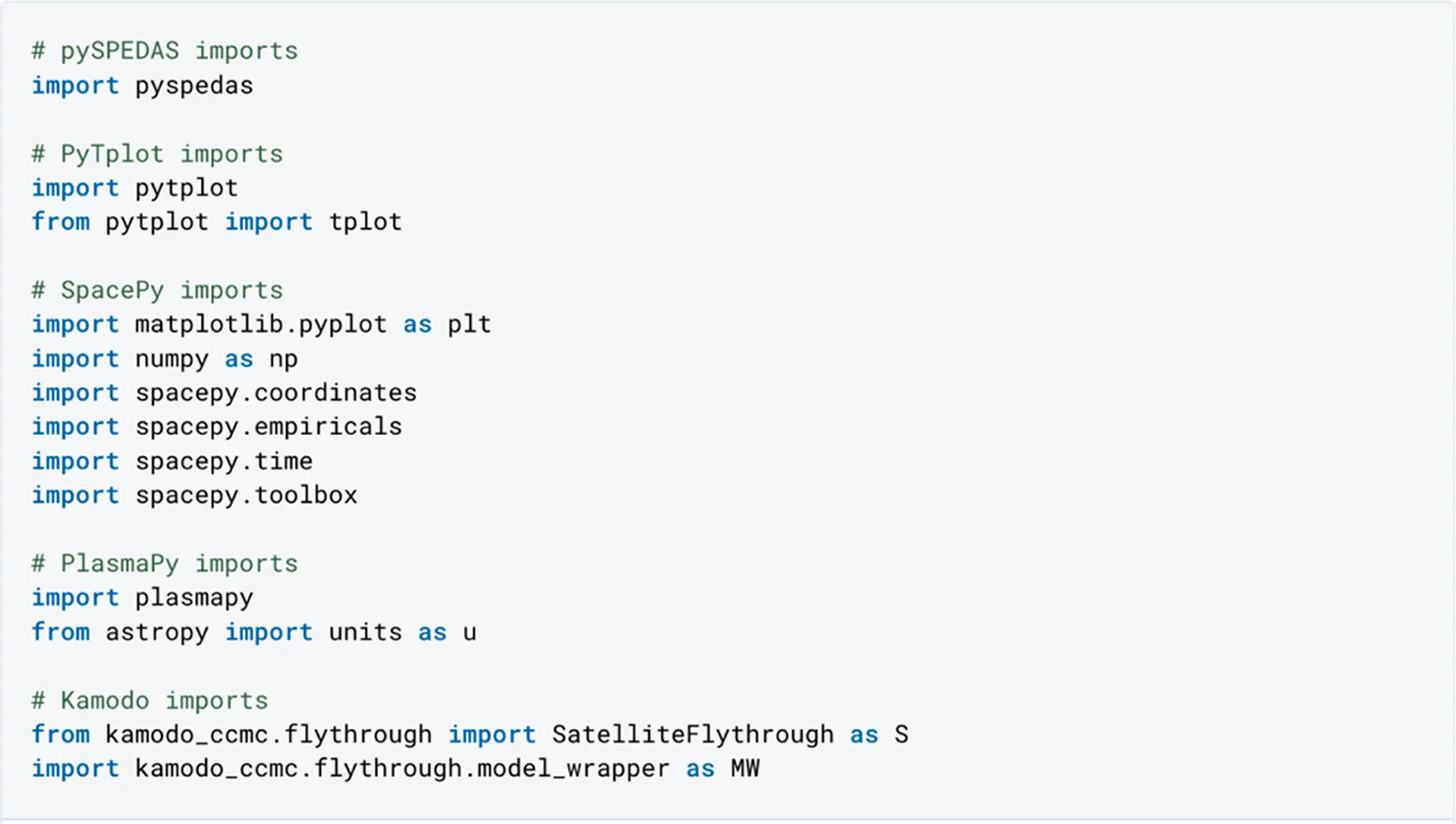
First, we need to import everything. We import pyspedas to load the MMS data and tplot from pytplot to plot it. Then we configure the necessary CDF library environment variables and make sure we have the solar wind data updated in our “.spacepy/” directory before importing the spacepy modules relevant to our magnetopause location calculations (plus numpy and matplotlib). We import plasmapy (plus astropy units) to augment our detections of magnetopause crossings. Finally, we import the kamodo modules relevant to performing our model flythrough.

2.2 Get MMS data

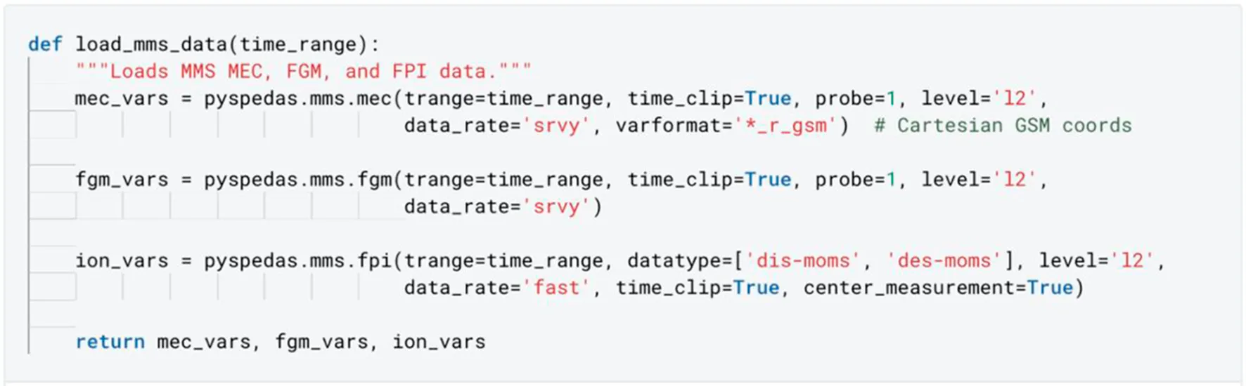
We retrieve MMS data using pySPEDAS for the time range specified in the trange variable. Note that pySPEDAS can retrieve data from any supported project (pySPEDAS 2022b) and that trange can be adjusted to any time range. The data gets downloaded into the pydata directory. No download is necessary if the data is already in the directory, such as ours is.

2.2.1 Set the time range for loading the data

2.2.2 Load the MEC, FGM and DIS data from pySPEDAS

Data can be loaded by calling pyspedas.mission.instrument() with options set via keyword arguments. For example, MEC data can be loaded by calling pyspedas.mms.mec(). There is, by default, a prompt to enter a science data center (SDC) username (which could be blank) before getting the MMS data. We avoid the prompt by creating an mms_auth_info.pkl file during our initialization. Data automatically gets loaded into Tplot variables upon loading (PyTplot 2022b).

MMS ephemeris and coordinates (MEC) data

These data show the spacecraft location at the times of the magnetopause crossings.

Fluxgate magnetometer (FGM) data

These data show the magnetic field as the spacecraft crosses the magnetopause.

Ion moments from the fast plasma investigation (FPI) data

These data show how the ion population changes as the spacecraft crosses the magnetopause.

2.3 Compare MMS data to an empirical model

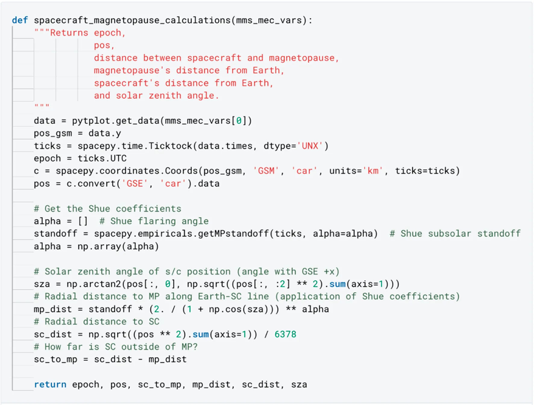
We use SpacePy to calculate where our MMS spacecraft is in relation to the magnetopause. SpacePy implements the empirical magnetopause model of Shue et al. (1998). A simple function supports calculating positions in the equatorial plane. For the out-of-plane calculations used here, more flexible functions are available. Upstream solar wind outputs, which are required for the model, are supported via SpacePy’s omni module using the OMNI data stored in our “.spacepy/” directory. We first perform the calculations then plot the results to visualize them.

SpacePy can work with other empirical models which also offer plasmapause distance and last closed drift shell as outputs.

2.3.1 Perform SpacePy calculations with MMS data

2.3.2 Detect magnetopause crossings

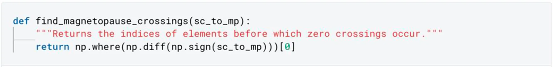
Since we can calculate the distance between the spacecraft and the magnetopause, we can find crossings by collecting the indices where that distance crosses 0 (i.e., changes sign):

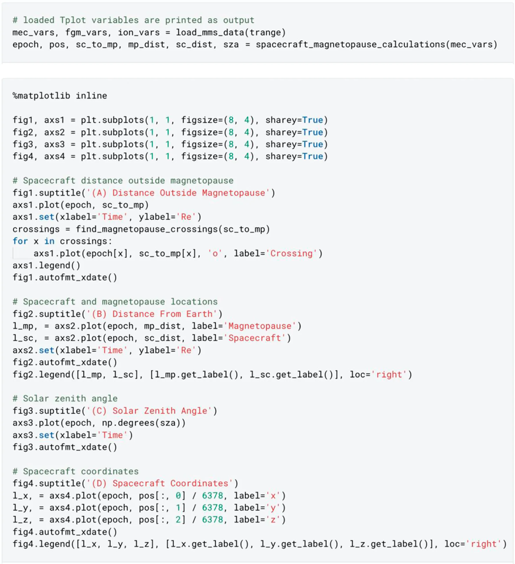
2.3.3 Plot distance outside magnetopause, spacecraft and magnetopause locations, and solar zenith angle

The following blocks of code plot each for our time range, using the helper functions we have so far defined.

2.4 Augment comparison with plasma parameters

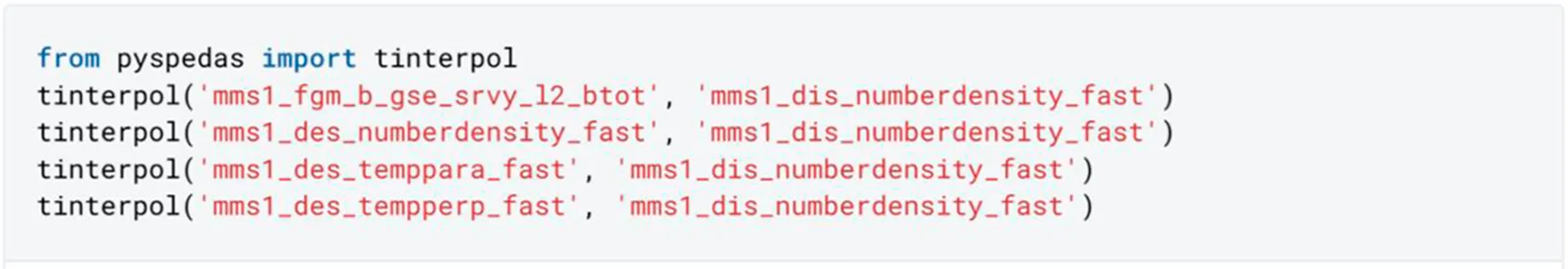
We use PlasmaPy to calculate various plasma parameters from the MMS data to help detect when MMS crosses the magnetopause boundary. Note that we calculate only a subset of the parameters PlasmaPy supports (PlasmaPy 2022a). The MMS data is retrieved from its Tplot variables and goes through some preparation before PlasmaPy can use it. We interpolate to a common set of times using the tinterpol function from pySPEDAS. We calculate the total temperature from the two temperature components given to us. And, lastly, we add Astropy units to the data (Astropy, 2022). Once we have these plasma parameters, we can plot them and visually compare them to plots of the MMS data. If the plots show sudden dramatic changes around a particular time, we can be reasonably confident that a magnetopause crossing happened then.

2.4.1 Prepare data for plasmaPy

2.4.1.1 Interpolate to a common set of times

We need to interpolate the B-field and DES (electron) data to the DIS (ion) time stamps. Note that tinterpol creates a new Tplot variable containing the interpolated output with the suffix ‘-itrp'.

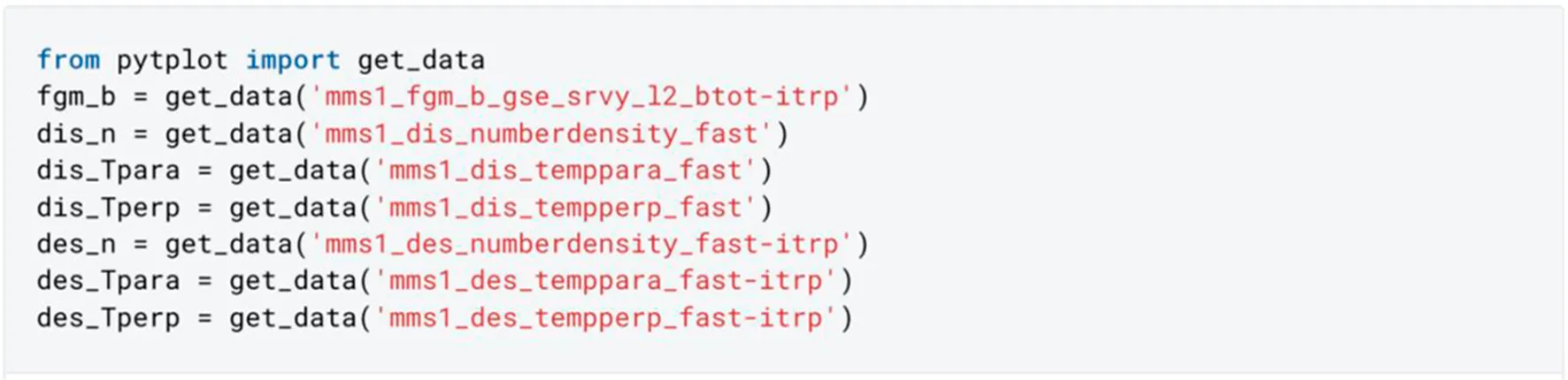
2.4.1.2 Extract the data values

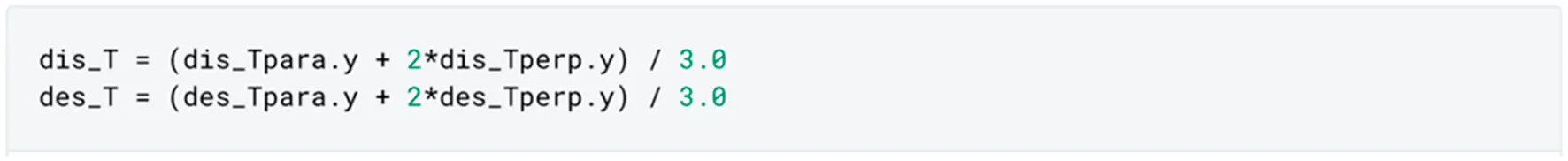
2.4.1.3 Calculate temperature

Temperature data released by the FPI team come as parallel and perpendicular components, but we need the total temperature. For details on this calculation, see the FPI Data Product Guide (LASP, 2022).

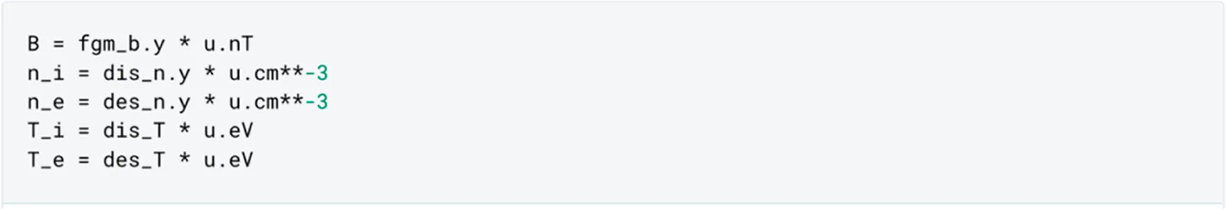
2.4.1.4 Add units to the data

PlasmaPy requires us to specify the units of the data using Astropy units.

2.4.2 Calculate plasma parameters

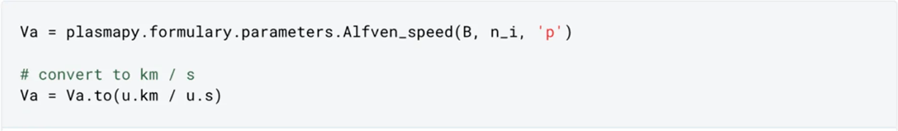
2.4.2.1 Alfvén speed

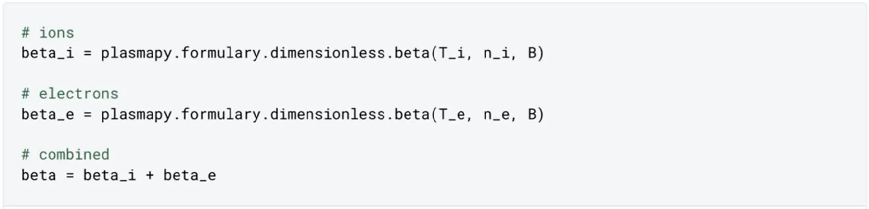
2.4.2.2 Plasma beta

2.4.2.3 Ion inertial length

2.4.2.4 Debye length

2.4.2.5 Ion gyrofrequency

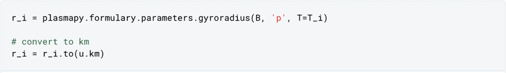
2.4.2.6 Ion gyroradius

2.4.2.7 Bohm diffusion coefficient

2.4.2.8 Lower hybrid frequency

2.4.2.9 Upper hybrid frequency

2.4.3 Generate plots with PyTplot

We can plot the calculated the plasma parameters with PyTplot.

2.4.3.1 Save the data in tplot variables

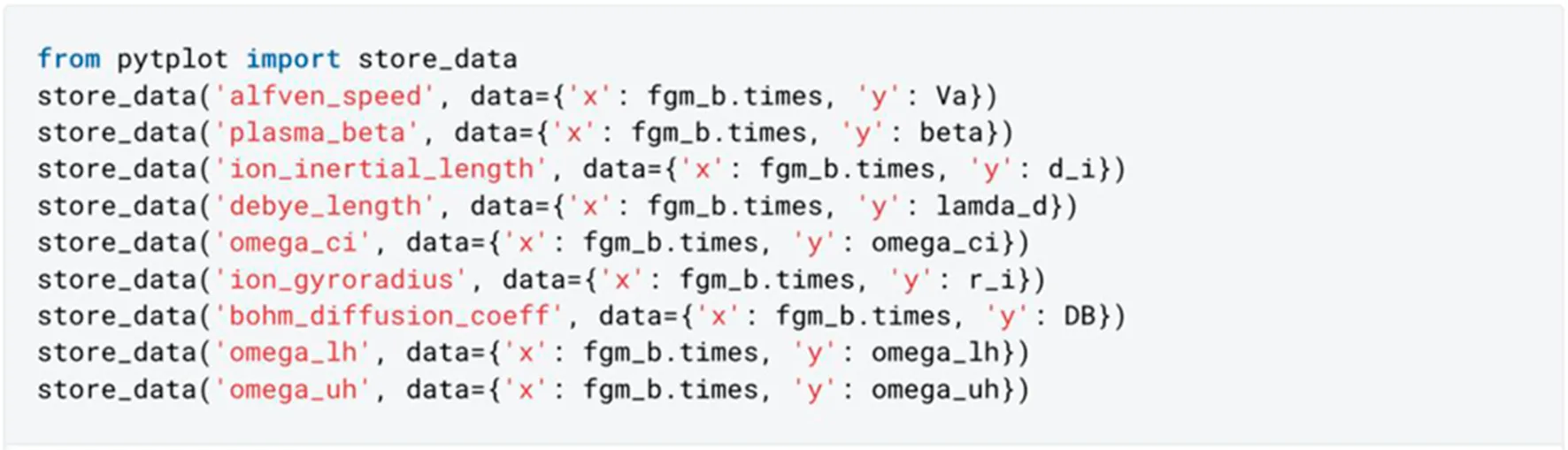
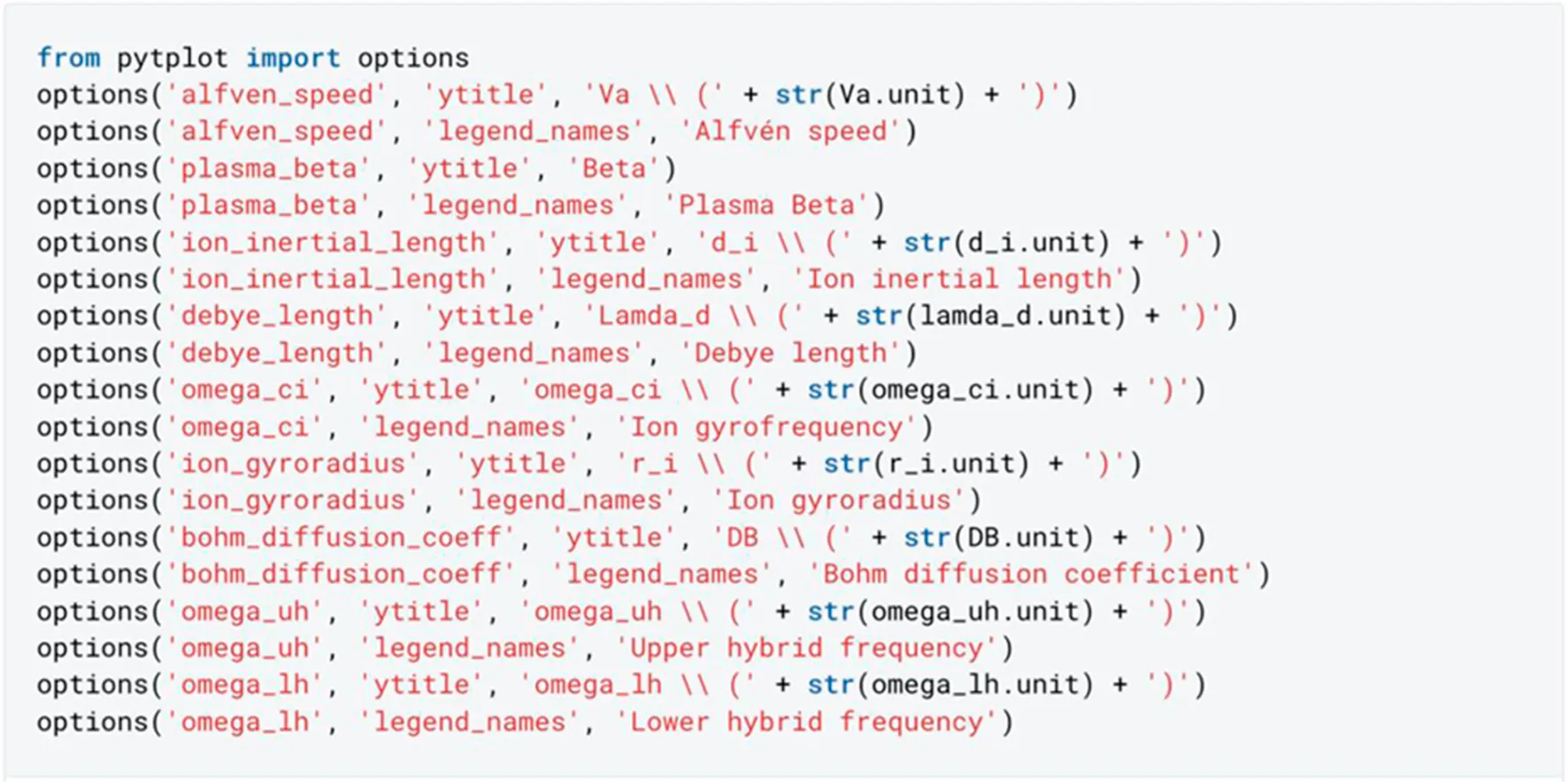
2.4.3.2 Set some plot metadata

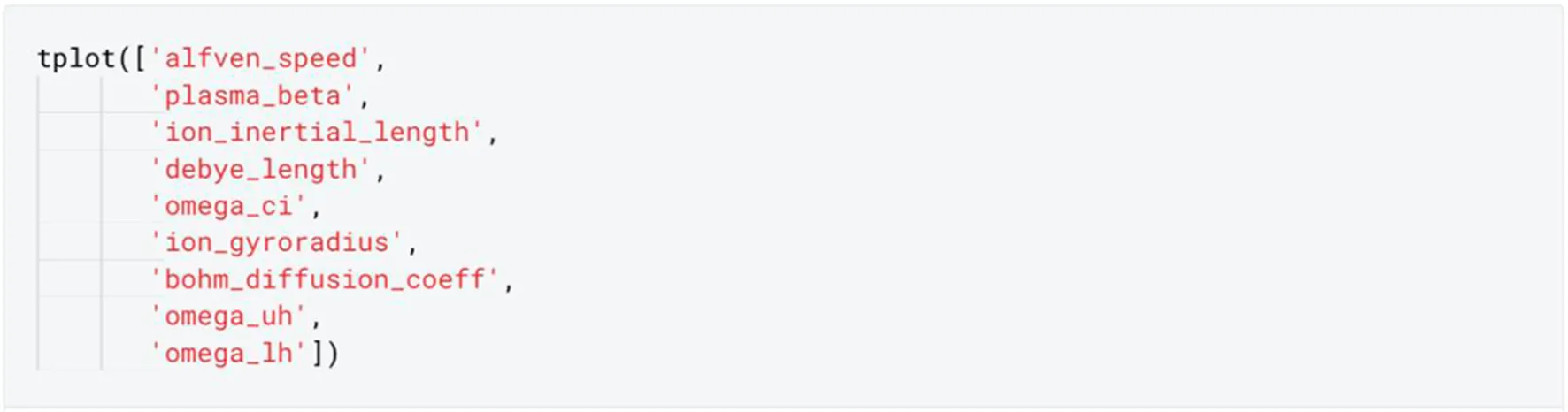
2.4.3.3 Plot the plasma parameters

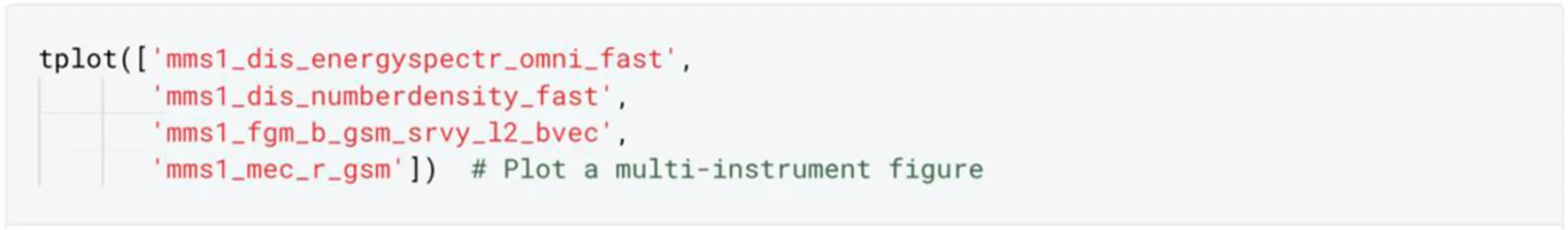
2.4.3.4 Plot the MMS data

2.4.4 Visual comparison

We can identify magnetopause boundary crossings in our data by looking for sudden changes around particular times. Both Figure 2 and Figure 3 show dramatic visual changes between 13:00–14:00 and spikes just before 15:00. These indicate at least two magnetopause crossings. If we compare these times with the earlier plot of a predicted crossing, Figure 4, we find a disagreement. The Shue et al. model predicted a crossing would have happened close to 16:00. Therefore, we can conclude the magnetopause was farther from Earth than the Shue et al. model predicted.

FIGURE 2

FIGURE 2. Time series plots showing (A) the distance between the MMS spacecraft and the modeled magnetopause, (B) the distances between the Earth and both the MMS spacecraft and the modeled magnetopause, (C) the solar zenith angle, and (D) the X, Y, and Z Cartesian coordinates of the MMS spacecraft. Note how plot (A) shows a predicted magnetopause crossing slightly before 16:00.

FIGURE 3

FIGURE 3. Time series plots showing the calculated plasma parameters. Note the dramatic visual changes between 13:00–14:00 and the spikes just before 15:00.

FIGURE 4

FIGURE 4. Time series plots showing the observed MMS data. Note the dramatic visual changes between 13:00–14:00 and the spikes just before 15:00.

2.5 Compare MMS data to a physics-based model

We use Kamodo to virtually fly the MMS spacecraft through the OpenGGCM magnetosphere model (Ringuette et al., 2022). Note that Kamodo’s flythrough capability provides access to various physics-based models and works on a variety of model types, not just magnetospheric models. See Kamodo’s flythrough documentation for more information (Kamodo 2022e). The choice of model is specified with a String variable (Kamodo 2022d). Run MW.Choose_Model(‘’) to see which Strings are allowed. A writable path to the model data files must be given to the ModelFlythrough function. The path must be writable because, upon running the ModelFlythrough function, Kamodo adds a CSV file to that directory which will have all available time ranges covered by the model’s data files.

2.5.1 Perform model flythrough with kamodo

2.5.1.1 Specify the model

2.5.1.2 See what variable names are available from the model

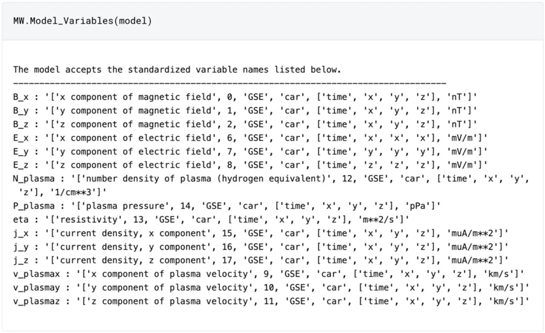
Note: although the model accepts all the variable names above, we have only populated our model files with data for B_x, B_y, and B_z to conserve space.

2.5.1.3 Prepare input variables

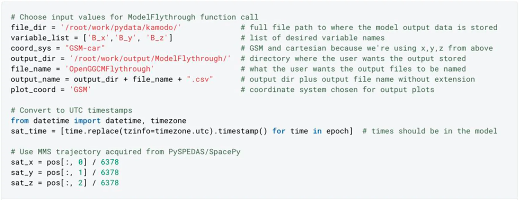
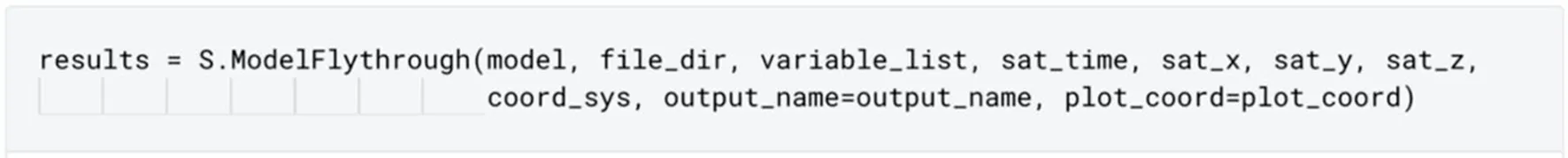
2.5.1.4 Perform the flythrough

The numeric results of this flythrough are exported to a file we named with the output_name variable. If a file by that name already exists, the ModelFlythrough function tells the user through an error message in order to prevent them from accidentally overwriting previous results. If the results have already been exported, they can be read from the file with a reader function as shown below.

Run ModelFlythrough with user-supplied trajectory to generate results:

If results have been previously generated, use the data import function to reload them:

2.5.1.5 Interact with flythrough plots

After the flythrough completes, the output plot files are exported to the directory output_dir; open them in a separate browser window for interactivity—nothing will open here. Both 3D and 1D plots are generated (Figures 5, 6).

FIGURE 5

FIGURE 5. A screenshot of a 3D plot produced by the Kamodo flythrough.

FIGURE 6

FIGURE 6. A screenshot of a 1D plot produced by the Kamodo flythrough.

3D plots will look like:

1D plots will look like:

2.5.2 Visual comparison

We now have values from a model of the magnetic field components measured by our MMS spacecraft. We can plot the modeled and observed values together to see how accurate the model is.

We do so using Kamodo’s built-in plotting capability, rather than matplotlib, because it produces interactive plots with very little code. We “Kamodofy” the results before we can plot them. “Kamodofication” is a concept Kamodo uses to “functionalize” callable functions, something that allows many problems in scientific data analysis to be posed in terms of function composition and evaluation. See the Kamodofication documentation for details about this concept (Kamodo 2022c).

Note that the model data files we use contain only the variables output by MW.File_Variables(model, file_dir) as compared to the full list of variables listed by MW.Model_Variables(model). We included only magnetic field component variables in our model data to conserve space, but OpenGGCM can model any of the full list of variables. Any of the modeled variables can be compared to the corresponding observed ones.

2.5.2.1 Extract the modeled and observed magnetic field components

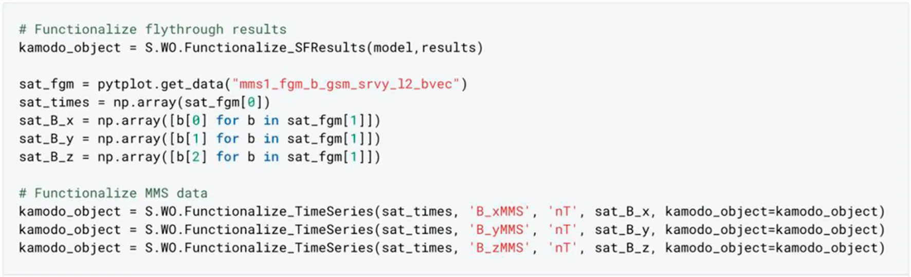
2.5.2.2 Plot the modeled and observed magnetic field components

The three plots in Figure 7, Figure 8, and Figure 9 show how well the OpenGGCM model simulates our real-world data. Recall that our model was intentionally generated at a coarse resolution to save storage space, so the simulation is only a rough approximation.

FIGURE 7

FIGURE 7. Time series plot of the observed B_x magnetic field component (blue) with the modeled one (red).

FIGURE 8

FIGURE 8. Time series plot of the observed B_y magnetic field component (blue) with the modeled one (red).

FIGURE 9

FIGURE 9. Time series plot of the observed B_z magnetic field component (blue) with the modeled one (red).

The sudden increases in B_x, B_y, and B_z in blue indicate that the MMS spacecraft transitioned from the magnetosheath (high plasma density, lower magnetic field strength) into the magnetosphere (low density, high magnetic field strength). The 10-min samples from the OpenGGCM model roughly follow the trend of the magnetosheath magnetic field. After about 13:40, when the satellite is in the magnetosphere, the model seems to predict that the satellite is still in the magnetosheath until about 14:50. In Figure 8, we see that the satellite moves about 0.25 R_E/hour in X towards the Earth. Encountering the magnetosphere in the sampling of the model outputs translates to an under-estimation of the magnetopause position in X by about 0.3 R_E. Confirmation of such an estimate, however, would require considerably higher temporal and spatial model resolution.

3 Results

In this work, we have described how open science principles guided the process of making this first executable paper in Heliophysics. The effort required for this process was sustainable and demonstrated how scientists and software developers can work together to more easily produce research of this quality and reproducibility. In presenting this example of our workflow, we showed that, during the time range used, the magnetopause was farther from Earth than the Shue et al. model predicted. We also showed how well the OpenGGCM model simulated the magnetic field components measured by MMS. By building this work into an executable paper, we have enabled not only direct reproducibility, but also made it so that anyone can easily build upon these results. We encourage others in our community to use this work as a launching point for their own research.

The open-source Python packages in our workflow (pySPEDAS, SpacePy, PlasmaPy, PyTplot, and Kamodo) made the analysis simple and guarded against reinventing the wheel. They constitute a great improvement over the outdated paradigm of siloed scientists writing scripts that ultimately never leave their machines. By using these packages in this format, we have lowered the barriers for others to reproduce our work. All they must do is run the same functions from the same package versions with the same data. The executable version of this paper makes that task trivially easy (all it takes is a few button clicks) due to the containerization provided by the Deepnote platform. Moreover, because our paper unambiguously showed what code to run when—something a generalized description of our method would have lacked—we prevented others from accidentally coming up with “false cognate” solutions that would not directly replicate our work. We promote this novel paper format as a vital supplemental tool to improve the reproducibility of traditional papers.

4 Discussion

There is some poetry in a newer organization like PyHC using a new platform like Deepnote to make a new kind of paper. But there are already well-established alternatives to Deepnote that may be more appropriate for other kinds of work. We discuss these alternatives in “Supplementary Appendix B” to guide the reader in their choice of platform. We note it is possible to create and share executable papers with any of these platforms. The decision of which platform to use may ultimately come down to the level of effort the authors are willing to put in. For example, the platform’s file size limits will be a crucial consideration for most projects since most platforms do not offer enough persistent storage space to hold hundreds of gigabytes. If the research requires a large amount of data, the authors might want to use a platform like JupyterLab where the executable paper could be shared from their own servers, rather than a platform like Deepnote which does not come with that much storage space. The trade-off would be the effort required to maintain the servers.

Now that we have published this executable paper, it is our responsibility to maintain it indefinitely. If anything breaks, we have to fix it and then update the DOI if necessary. We have no way of knowing how much work this will turn out to be. However, the likelihood of anything breaking was dramatically reduced by putting 100% of our research materials in our container. We predict the main thing to watch out for will be problems with future versions of the underlying containerization software. Still, this is a drawback to this paper format and a leading reason why it cannot yet replace traditional papers. Significant new infrastructure will be needed if the scientific community ever decides to dedicate themselves to executable papers. But the format offers too many reproducibility benefits to ignore it.

We encourage all researchers to make executable versions of their papers, but especially Heliophysics researchers who use Python. PyHC’s goal, after all, is to bring such people into our community and unite them. Imagine with us: a beautiful world where all Python-using Heliophysicists use the same Python packages when doing the same work to answer the same questions. Furthermore, they share executable versions of their resulting research papers, giving them all a faster launching point to reproduce and use each other’s work. At the same time, they are satisfying the necessary requirements to do responsible open science. If you like this vision, join us! [See our contact page (Polson and Barnum 2022)]. Our field would be more on the same page, making it easier to answer our questions about the Universe. And is that not the whole point of why we do this research in the first place?

4.1 Future work

At present, our OpenGGCM data is too coarse for deep scientific analysis. We would like to improve our model data to better capture nuances at the magnetopause boundary. For example, we could increase the 10-min cadence to, say, one second. Or, to avoid increasing the file sizes excessively, the model output conversion step to NetCDF files could include the possibility to extract a subset of the model data in space around the satellite location.

Such improvements could potentially make the data files too large to fit in this container despite the mentioned possibilities to decrease it, but if it does, we could start storing everything in a container that we host ourselves. Once we have this better model data, we will shift to focus on scientific applications of our workflow and compare more magnetosphere models to spacecraft data. We plan to publish an in-depth comparison that will examine more time ranges, spacecrafts, and models and delve deeper into the relevant science questions.

The approach used to create this paper was valuable and sustainable. We will do more work in the future to share this approach in an effort to convince our field to adopt our practices. This will include presenting talks about our approach at conferences and organizing PyHC activities around the matter (such as telecon presentations and hackathons during our biannual community meetings). We will also investigate matters of interoperability with other executable papers and how to describe our executable papers with metadata. Finally, we will offer direct support to any researchers who contact us for guidance.

Data availability statement

All data used in this work are stored inside the Docker container that houses this executable paper (https://doi.org/10.5281/zenodo.7412347). Further inquiries can be directed to the corresponding author.

Author contributions

All authors contributed to manuscript revision, read, and approved the submitted version. Individual contributions are described in Supplementary Appendix A.

Funding

This work is supported by NASA under award 80NSSC22K0326, managed by the Goddard Space Flight Center.

Acknowledgments

We gratefully acknowledge Darren De Zeeuw for valuable discussions and code contributions to the Kamodo project in support of this work. We gratefully acknowledge Bryan Harter for technical assistance and code contributions to the PyTplot project in support of this work. Simulation results have been provided by the Community Coordinated Modeling Center at Goddard Space Flight Center through their publicly available simulation services (https://ccmc.gsfc.nasa.gov). The OpenGGCM model was developed by J. Raeder at the University of California, Los Angeles, and T. Fuller-Rowell at NOAA/SEC. The RCM model was developed by R. K. Jaggi, R. A. Wolf, R. W. Spiro, and F. J. Rich at Rice University and at the Phillips Laboratory of the United States Air Force (Wolf et al., 2016). The Shue et al. model was developed by J.-H. Shue et al. at Nagoya University in Toyokawa, Japan. We thank the Magnetospheric Multiscale Mission team for the use of data from their instruments, the OMNI team for their assimilative solar wind datasets, and J. Gannon for USGS Dst data. We also thank contributors to the NumPy, SciPy, and matplotlib tools, and our SpacePy co-authors at Los Alamos National Laboratory. And lastly, we thank the Frontiers Design Team for the special treatment and extra effort needed to typeset this paper in its novel format.

Conflict of interest

RR was employed by ADNET Systems Inc.

The remaining authors declare that the research was conducted in the absence of any commercial or financial relationships that could be construed as a potential conflict of interest.

Publisher’s note

All claims expressed in this article are solely those of the authors and do not necessarily represent those of their affiliated organizations, or those of the publisher, the editors and the reviewers. Any product that may be evaluated in this article, or claim that may be made by its manufacturer, is not guaranteed or endorsed by the publisher.

Supplementary material

The Supplementary Material for this article can be found online at: https://www.frontiersin.org/articles/10.3389/fspas.2022.977781/full#supplementary-material

Footnotes

¹Link to the executable version of this paper on Deepnote: https://deepnote.com/@shawn-polson/PyHC-Paper-101b9646-3fd0-4978-a48e-a4f3e708a0ac.

²DOI to the files of the executable version of this paper on Zenodo: https://doi.org/10.5281/zenodo.7412347.

³OpenGGCM input parameters:• run ID: Yihua_Zheng_031022_1• model: OpenGGCM• version: 5.0• IM_model: RCM• IM_version: 1.0• cs_input: GSM• cs_output: GSE• event_date: 16 October 2015• start_time: 2015/10/16 11:30• end_time: 2015/10/16 17:00• run_type: event• solarwind: var• sw_source: OMNI• despike solar wind data: 0• despike: threshold (sigmas): 3• despike: number of samples: 5• setting option for Bx: user• constant-Bx: 0• By-coefficient: 0• Bz-coefficient: 0• b_abs: 2.19• b_angle: 123.13• iono_conductance: auroral• Pedersen Conductance: default• Hall Conductance: default• f10.7: 108.4.

⁴The OpenGGCM model was run with a low-resolution grid (“dayside emphasis grid with 3,500,000 cells” with 355 × 100 × 100 cells) in the simulation domain extending from -350 to 33 R_E in X_GSM, and up to 49 R_E in |Y_GSE| and |Z_GSE| with a 0.3 R_E resolution around the Earth. During the packaging of magnetosphere model outputs into Kamodo, NetCDF files were reduced to only include magnetic field components (B_x, B_y, B_z) at a 600-s time cadence to limit model outputs to 1.6 GB. The near-Earth boundary conditions at 2.5 R_E distance includes 100 particles/cm³, a temperature of 100 eV, and a shielding latitude of 45° in the ionosphere electric field potential solver.

References

Akhlaghi, M. reproducible-paper. GitLab. Available at: https://gitlab.com/makhlaghi/reproducible-paper.

Google Scholar

Alm, L., Argall, M. R., Torbert, R. B., Farrugia, C. J., Burch, J. L., Ergun, R. E., et al. (2017). EDR signatures observed by MMS in the october 16 event presented in a 2D parametric space. American Geophysical Union.

Google Scholar

American Society for Cell Biology (2015). Task force on scientific reproducibility calls for action, reform: Public concern about reproducibility is legitimate, scientists must respond effectively, say experts. Science Daily. Available at: https://www.sciencedaily.com/releases/2015/07/150715090508.htm.

Google Scholar

Astropy, (2022). Units and quantities. Available at: https://docs.astropy.org/en/stable/units/index.html (Accessed April 8).

Google Scholar

Bajpai, V., et al. (2017). Challenges with reproducibility.” in Proceedings of the reproducibility workshop.

CrossRef Full Text | Google Scholar

Baker, M. (2016a). 1, 500 scientists lift the lid on reproducibility. Nature 533, 452–454. doi:10.1038/533452a

PubMed Abstract | CrossRef Full Text | Google Scholar

Baker, M. (2016b). Stat-checking software stirs up psychology. Nature 540, 151–152. doi:10.1038/540151a

PubMed Abstract | CrossRef Full Text | Google Scholar

Binder, (2022). Binder documentation. Binder User Guide. Available at: https://mybinder.readthedocs.io/en/latest/.

Google Scholar

Burch, J. L., Torbert, R. B., Phan, T. D., Chen, L.-J., Moore, T. E., Ergun, R. E., et al. (2016). Electron-scale measurements of magnetic reconnection in space. Science 352 (6290), aaf2939. doi:10.1126/science.aaf2939

PubMed Abstract | CrossRef Full Text | Google Scholar

Cacho, J. R., and Taghva, K. (2020). The state of reproducible research in computer science.” in 17th International Conference on Information Technology–New Generations (ITNG 2020). Springer.

CrossRef Full Text | Google Scholar

CodaLab (2020). Executable papers. CodaLab Worksheets Documentation. Available at: https://codalab-worksheets.readthedocs.io/en/latest/Executable-Papers/.

Google Scholar

Community Coordinated Modeling Center (2022). OpenGGCM model information. NASA GSFC. Available at: https://ccmc.gsfc.nasa.gov/models/modelinfo.php?model=OpenGGCM.

Google Scholar

Deepnote, (2022). Data science notebook for teams. Deepnote. Available at: https://deepnote.com.

Google Scholar

Docker, (2022). What is a container? Docker. Available at: https://www.docker.com/resources/what-container/. (Accessed April 8).

Google Scholar

Egedal, J., Le, A., William, S., and Daughton, S. (2017). The kinetic structure of the electron diffusion region observed by MMS during asymmetric reconnection. AGU Fall Meeting, SM22B–01.

Google Scholar

Elsevier, Executable Papers - improving the article format in computer science. Elsevier News. Available at: https://www.journals.elsevier.com/the-journal-of-logic-and-algebraic-programming/news/introducing-executable-papers.

Google Scholar

Fanelli, D. (2018). Opinion: Is science really facing a reproducibility crisis, and do we need it to? Proc. Natl. Acad. Sci. U. S. A. 11511, 2628–2631. doi:10.1073/pnas.1708272114

CrossRef Full Text | Google Scholar

Foster, (2022). What is open science? Introduction. FOSTER Open Science. Available at: https://www.fosteropenscience.eu/content/what-open-science-introduction.

Google Scholar

Gentemann, C., Ivey, Y., Crawford, S., Baynes, K., Murphy, K., Ward, K., et al. (2021). NASA open-source science initiative: Transform to open science (TOPS). Zenodo. October 29. doi:10.5281/zenodo.5621674

CrossRef Full Text | Google Scholar

Google Research (2022a). Colaboratory frequently asked questions.” Google Colab. Google. Available at: https://research.google.com/colaboratory/faq.html.

Google Scholar

Google Research (2022b). Welcome to colaboratory. Google Colab. Google. Available at: https://colab.research.google.com/ (Accessed April 8).

Google Scholar

Jupyter, (2022). Jupyter NotebookProject Jupyter. Available at: https://jupyter.org/.

JupyterLab, (2022). JupyterLab documentation. Jupyter. Available at: https://jupyterlab.readthedocs.io/en/stable/(Accessed April 8).

Google Scholar

Kamodo, (2022a). kamodo-core.” GitHub. Available at: https://github.com/EnsembleGovServices/kamodo-core (Accessed April 8).

Google Scholar

Kamodo, (2022b). GitHub. Available at: https://ccmc.gsfc.nasa.gov/Kamodo (Accessed April 8).

Google Scholar

Kamodo, (2022c). Kamodofication tutorial.” CCMC. Available at: https://ccmc.gsfc.nasa.gov/Kamodo/notebooks/Kamodofying_Models/ (Accessed April 8).

Google Scholar

Kamodo, (2022d). notebooks. GitHub. Available at: https://github.com/nasa/Kamodo/tree/master/notebooks (Accessed April 8).

Google Scholar

Kamodo, (2022e). model_wrapper.py.” GitHub. Available at: https://github.com/nasa/Kamodo/blob/b8823e5e37875f4b8aae473551b76a4d9c8aef7a/kamodo_ccmc/flythrough/model_wrapper.py#L50 (Accessed April 8).

Google Scholar

Lasp, (2022). FPI data product guide. Available at: https://lasp.colorado.edu/galaxy/pages/viewpage.action?pageId=37618954 (Accessed April 8).

Google Scholar

Lasser, J. (2020). Creating an executable paper is a journey through Open Science. Commun. Phys. 31, 143. doi:10.1038/s42005-020-00403-4

CrossRef Full Text | Google Scholar

Merriam-Webster, (2022). Magnetopause definition & meaning. Merriam-Webster. Available at: https://www.merriam-webster.com/dictionary/magnetopause (Accessed April 8).

Google Scholar

Morley, S. K., et al. (2011). “Spacepy - a Python-based library of tools for the space sciences,” in Proceedings of the 9th Python in science conference. SciPy 2010). doi:10.25080/Majora-92bf1922-00c

CrossRef Full Text | Google Scholar

NASA (2022). Magnetospheres.” NASA science. NASA. Available at: https://science.nasa.gov/heliophysics/focus-areas/magnetosphere-ionosphere (Accessed April 8).

Google Scholar

Nelson, N. C., Ichikawa, K., Chung, J., and Malik, M. M. (2021). Mapping the discursive dimensions of the reproducibility crisis: A mixed methods analysis. Plos one 167 (2021), e0254090. doi:10.1371/journal.pone.0254090

CrossRef Full Text | Google Scholar

Niehof, J. T., et al. (2022). SpacePy: Tools for space science applications. doi:10.5281/zenodo.3252523

CrossRef Full Text | Google Scholar

PlasmaPy, (2022a). Plasma parameters. Available at: https://docs.plasmapy.org/en/stable/formulary/parameters.html (Accessed April 8).

Google Scholar

PlasmaPy, (2022b). PlasmaPy.” GitHub. Available at: https://github.com/PlasmaPy/plasmapy (Accessed April 8, 2022).

Google Scholar

Polson, S., and Barnum, J. (2022). Heliopython. Available at: https://heliopython.org/contact/ (Accessed April 8, 2022).

Google Scholar

PyHC (2022a). Projects. Available at: https://heliopython.org/projects/ (Accessed April 8).

Google Scholar

PyHC (2022b). Python in Heliophysics community gallery. Available at: https://heliopython.org/gallery/generated/gallery/index.html (Accessed April 8).

Google Scholar

PyHC (2022c). Python in Heliophysics community (PyHC). Available at: https://heliopython.org (Accessed April 8).

Google Scholar

PyHC. (2022d). Python in Heliophysics community (PyHC) standards. (Accessed April 8). doi:10.5281/zenodo.2529131

CrossRef Full Text | Google Scholar

pySPEDAS (2022a). pySPEDAS. GitHub. Available at: https://github.com/spedas/pyspedas (Accessed April 8).

Google Scholar

pySPEDAS (2022b). Load routines. Available at: https://pyspedas.readthedocs.io/en/latest/projects.html (Accessed April 8, 2022).

Google Scholar

PyTplot (2022a). PyTplot. GitHubAvailable at: https://github.com/MAVENSDC/pytplot (Accessed April 8).

Google Scholar

PyTplot, (2022b). Tplot variables. Available at: https://pytplot.readthedocs.io/en/latest/tplot_variables.html (Accessed April 8).

Google Scholar

Qin, Z., Denton, R. E., Tsyganenko, N. A., and Wolf, S. (2007). Solar wind parameters for magnetospheric magnetic field modeling. Space weather. 5, 11. doi:10.1029/2006SW000296

CrossRef Full Text | Google Scholar

Ragan-Kelley, B., and Willing, C. (2018). “Binder 2.0-Reproducible, interactive, sharable environments for science at scale.” in Proceedings of the 17th Python in Science conference Editors F. Akici, D. Lippa, D. Niederhut, and M. Pacer 113–120.

Google Scholar

Reproducible Research How to make a paper reproducible? Available at: https://reproducibleresearch.net/how-to-make-a-paper-reproducible/.

Google Scholar

Ringuette, R., De Zeeuw, D., Rastaetter, L., and Pembroke, A. (2022). Kamodo's model-agnostic satellite flythrough: Lowering the utilization barrier for Heliophysics model outputs. Front. Astron. Space Sci. 9, 1005977. doi:10.3389/fspas.2022.1005977

CrossRef Full Text | Google Scholar

Shue, J.-H., Song, P., Russell, C. T., Steinberg, J. T., Chao, J. K., Zastenker, G., et al. (1998). Magnetopause location under extreme solar wind conditions. J. Geophys. Res. 103 (A8), 17691–17700. doi:10.1029/98ja01103

CrossRef Full Text | Google Scholar

SpacePy GitHub. Available at: https://spacepy.github.io (Accessed April 8, 2022).

Google Scholar

Vicente-Saez, R., and Martinez-Fuentes, C. (2018). Open science now: A systematic literature review for an integrated definition. J. Bus. Res. 88, 428–436. doi:10.1016/j.jbusres.2017.12.043

CrossRef Full Text | Google Scholar

Ware, A., and Roberts, D. A. (2019). The Python in Heliophysics community. Geophys. Res. Abstr. 21.

Google Scholar

Wolf, R. A., Spiro, R. W., Sazykin, S., Toffoletto, F. R., and Yang, J. (2016). Forty-seven years of the Rice convection model. doi:10.1002/9781119066880.ch17

CrossRef Full Text | Google Scholar