The predictive power of magnetospheric models for estimating ground magnetic field variation in the United Kingdom

1 Introduction

Research into the hazard posed by space weather events to in-orbit and ground-based technology has grown rapidly in recent years. Geomagnetic storms cause rapid fluctuations in the Earth’s magnetic field (B) resulting in the induction of geoelectric fields in the subsurface. These give rise to geomagnetically induced currents (GICs) which negatively affect high voltage power networks, pipelines and railways (Boteler, 1994; 2021; Boteler et al., 1998; Pirjola, 2000; Zhang et al., 2015; Rajput et al., 2021). Variations in the geomagnetic field can also affect navigation in directional drilling used in the oil and gas industry (Reay et al., 2005). The negative effects of extreme geomagnetic activity have been observed many times. The first recorded example is known as the Carrington event in 1859, which is believed to be the most severe magnetic storm ever observed (Chapman et al., 2020), causing significant interference with telegraph lines (Cliver and Dietrich, 2013; Hayakawa et al., 2019). Another example is the large storm from March 1989 which is considered one of the most significant magnetic storms of the 20th century, strongly affecting the northern regions of the United States and Europe. Geomagnetic disturbances caused transformer damage resulting in the collapse of the Hydro-Quebec power system, which left millions of people without power for several hours (Bolduc, 2002; Boteler, 2019). A more recent example is the moderate storm from February 2022, during which the majority of Starlink satellites launched into a very low orbit (200 km) were deorbited due to enhanced atmospheric drag. This event shows that even minor storms can have severe financial consequences (Dang et al., 2022). To prevent and mitigate such negative impacts, reliable space weather forecasting methods are essential for providing early warning to infrastructure operators.

Over the past decades, many space weather prediction models have been developed. They aim to simulate the complexity of the solar wind-magnetosphere-ionosphere coupling by solving the magnetohydrodynamic (MHD) equations. Many currently available models rely on solar wind parameters, obtained upstream of the Earth at the L1 Lagrange point by satellite, as their input which are then propagated further down into the Earth’s magnetosphere and ionosphere. Using post-processing tools and techniques, the magnetic field perturbations at a given location on the ground can be then estimated from snapshots of the field-aligned and ionosphere height-integrated currents produced by the simulations (Rastätter et al., 2014). Such MHD models are increasingly being used for operational services for predicting values of ground magnetic fields and to provide hazard assessments and warnings up to several hours in advance of an anticipated space weather event. Hence it is important to understand their performance, uncertainties and limitations, particularly as secondary and tertiary services become reliant on their forecasts. In general, the MHD approach is believed to correctly describe the large-scale interaction of solar wind with magnetosphere and ionosphere theoretically by using constant solar wind parameters and interplanetary magnetic field as input. With the availability of more and more observational data from ground-based and space-borne observatories, researchers have tried to model the responses of the magnetosphere to real-time observations by using data-driven global MHD simulations with realistic observed parameters as input. Feng and Feng (2020) present an overview of such global MHD models of magnetosphere, with the focus on numerical implementations.

The performance of such models has been assessed in multiple validation challenges and studies in the past, focusing mainly on large high latitude regions in the northern hemisphere during geomagnetically disturbed periods (Yu and Ridley, 2008; Pulkkinen et al., 2011; Rastätter et al., 2011; Pulkkinen et al., 2013; Rastätter et al., 2013; Welling et al., 2017; Kwagala et al., 2020). These studies use a variety of metrics to evaluate the performance of chosen models in replicating ground field variations, as well as their rate of change with time measured at selected ground magnetic observatories. However, less attention has been paid to low and mid-latitudes where the majority of the global population live and much of the potentially vulnerable infrastructure is located (Zhang et al., 2016; Oughton et al., 2019).

Large variations of the horizontal magnetic field component are the main driver of the resulting geoelectric field at the Earth’s surface (Bolduc et al., 1998; Viljanen et al., 2001; Smith et al., 2021). Since the induced electric field also depends on the relative geometry and properties of the power network, the orientation of the magnetic field (North-South, B_x, and East-West, B_y) should also be considered to provide more detailed and effective GIC forecast (Kelly et al., 2017). Therefore, in the work presented here, individual components B_x and B_y are the main focus, though the horizontal field $(B_H=\sqrt{B_x^2+B_y^2})$ is also considered. Accurate values of ground magnetic fields, particularly time-series, allow geoelectric fields and GICs to be computed with greater confidence through magnetotelluric transfer functions and models of the response of high voltage power grids to variation in ground electric field (Beggan et al., 2021).

The following section (Section 2) describes the validation setting, including the selected space weather events, location of the United Kingdom observatories and information about the MHD models investigated. Data-model comparison metrics selected for performance assessment are described in Section 3. The results and data-model comparison analysis can be found in Section 4, followed by a brief discussion and concluding remarks in Section 5.

2 Magnetohydrodynamic model validation setting

2.1 Selected geomagnetic storms

In this study, two of the largest geomagnetic storms from solar cycle 24 are investigated. The details and duration of each can be found in Table 1. Both selected events cover the most disturbed 24-h period of the respective storm. The severity of each event can be determined by various space weather indices. The planetary Kp index quantifies magnetic activity in the range from 0 to 9, where 0 describes quiet conditions and 5 or greater indicates a storm (Bartels et al., 1939). The Dst index describes the variation in the ring current intensity and is believed to reflect the global magnetic field reduction during storms. It is derived from the horizontal magnetic field component measured at four nearly equatorial magnetic observatories and the resulting Dst is calculated at 1 h intervals. Similarly to Dst, SYM-H index represents the symmetric part of the horizontal component but relies on data from six observatories instead, providing more even distribution in longitude. The resulting SYM-H is given in 1-min resolution. Detailed description of the differences between the two indices can be found in Wanliss and Showalter (2006). The values of selected indices for each event presented in Table 1 were acquired from World Data Center for Geomagnetism, Kyoto¹.

TABLE 1

TABLE 1. Details of the space weather events analysed.

Early September 2017 is considered one of the most geomagnetically active periods of solar cycle 24, where a significant number of sunspots caused several major flares and coronal mass ejections (CMEs). This period has been analysed in many studies, for example by Rodger et al. (2020); Clilverd et al. (2018); Dimmock et al. (2019); Qian et al. (2019); Piersanti et al. (2019); Simpson and Bahr (2021). Severe geomagnetic activity observed on the Earth was a consequence of multiple X-class and M-class solar flares that occurred on the 6th and 7th of September. In the following analysis we investigate the period associated with the sudden storm commencement caused by the solar shock arrival just after 23:00 UT on the 7th, when solar wind speed drastically increased.

The second event is another well-known storm, commonly referred to as the St. Patrick’s Day event. It is considered the first super geomagnetic storm of solar cycle 24. This storm was associated with a CME that occurred on 15 March 2015, reaching Earth on March 17th. Just like the September 2017 storm, this event is also a popular research topic within the space weather research community (Zhang et al., 2015; Carter et al., 2016; Guerrero et al., 2017; Huba et al., 2017; Divett et al., 2018; Ngwira et al., 2018).

2.2 Ground magnetic observatories

We use data from three United Kingdom geomagnetic observatories operated by the British Geological Survey: Hartland (HAD) in Devon, England; Eskdalemuir (ESK) in the Southern Uplands of Scotland and Lerwick (LER) in the Shetland Islands. Detailed location information for each of them can be found in Table 2 and on the map in Figure 1.

TABLE 2

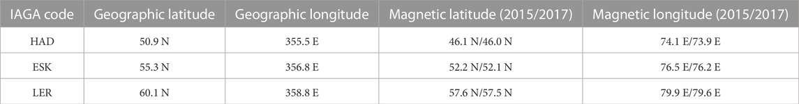
TABLE 2. Locations in degrees of the United Kingdom geomagnetic observatories, including both geographic and magnetic coordinates (magnetic coordinates are approximations calculated using the 13th generation IGRF at epoch 2015.25 and 2017.75, respectively).

FIGURE 1

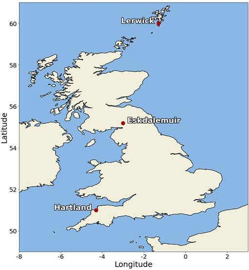
FIGURE 1. Map of the permanent United Kingdom geomagnetic observatories.

Ground magnetic field measurements, at minute-mean cadence, were obtained from the INTERMAGNET website². The quiet time average was removed from each data set by subtracting the mean value taken over the first 2 h of each time series to leave only the external field variations. Those data sets are then used as “ground truth” for comparison with simulated results.

2.3 Magnetohydrodynamic models

2.3.1 Space weather modeling framework

The Space Weather Modeling Framework (SWMF) was developed by the Center for Space Environment Modeling (CSEM) at the University of Michigan. It aims to simulate various domains of the Sun-Earth chain, and ultimately help predict space weather phenomena. This framework combines numerical models of various regions between the Sun and the Earth into a high-performance coupled model (Tóth et al., 2005). In this study, the global magnetosphere (GM) and its coupling to the inner magnetosphere (IM) are the main focus.

The model included in SWMF that describes the mentioned domains is the Block-Adaptive-Tree Solar-Wind Roe-Type Upwind Scheme (BATS-R-US) (Powell et al., 1999). The BATS-R-US code solves the ideal 3D MHD equations as well as semi-relativistic, Hall, multispecies and multifluid equations (Gombosi et al., 2002; Glocer et al., 2009). The governing equations for an ideal, non-relativistic, compressible plasma, written in primitive variables, represent a combination of the Euler formulas of gas dynamics and Maxwell equations of electromagnetism. BATS-R-US uses the block-based adaptive mesh refinement (AMR) technique with a finite volume form using numerical methods related to Roe’s Approximate Riemann Solver. A variety of different grids are available, as well as explicit, implicit and point-implicit time stepping options (Zeeuw et al., 2004; Glocer et al., 2009; 2013; Ridley et al., 2016). Detailed description of the code and the adaptive blocks technique can be found in papers by Zeeuw et al. (2000) and Stout et al. (1997).

The SWMF/GM uses solar wind plasma data (density, velocity, temperature and magnetic field) in Geocentric Solar Magnetospheric (GSM) coordinates as input, which are then propagated from the L1 Lagrange satellite position to the sunward boundary of the simulation domain. The Earth’s magnetic field is represented by a dipole with either a fixed orientation or updated axis orientation and co-rotating inner magnetospheric plasma during the simulation run. The outputs provided by SWMF/GM include plasma parameters, magnetic field and electric currents. In this study the following SWMF configurations were used for both events:

• SWMF v20180525, high-resolution grid with 9,623,552 cells,

• SWMF v20180525 coupled with RCM, high-resolution grid with 9,623,552 cells.

2.3.2 Open geospace general circulation model

The Open Geospace General Circulation Model (OpenGGCM) is a global coupled model of Earth’s magnetosphere, ionosphere and thermosphere. In the magnetospheric part, the model solves the resistive MHD equations as an initial-boundary-value problem. The ionosphere potential solver closes the magnetospheric field-aligned currents in the ionosphere, effectively combining magnetospheric convection with ionospheric convection. The magnetospheric module was later improved by coupling with the ionosphere-thermosphere system modelled by the NOAA CTIM [Coupled Thermosphere Ionosphere Model (Fuller-Rowell et al., 1996)]. This addition maps the field-aligned currents into the ionosphere, computes the ionospheric potential and electron precipitation parameters as well as Hall and Pedersen conductances (Raeder et al., 2008; Raeder et al., 2017; Cramer et al., 2017). Similarly to SWMF, OpenGGCM uses solar wind plasma and magnetic field parameters as input, which are propagated to the upstream simulation boundary. The simulated Earth’s magnetic field is approximated by a dipole with fixed orientation during the entire simulation run. The following configurations of the OpenGGCM simulation will be analysed for both events:

• OpenGGCM 5.0, overview grid with 7 M cells,

• OpenGGCM 5.0 coupled with RCM, overview grid with 7 M cells.

2.3.3 Lyon-Fedder-Mobarry

The Lyon-Fedder-Mobarry (LFM) global magnetospheric simulation code was first developed around 1985 and improved over the years with higher resolving power transport, adapted grid, high Alfvén speed, low plasma β, and high magnetic field as well as an integral ionospheric model (Lyon et al., 2004). The Magnetosphere-Ionosphere Coupler/Solver (MIX) code provides the LFM model with the ionospheric electrostatic potential solution and electric field inner boundary condition information (Merkin and Lyon, 2010). The thermosphere-ionosphere electrodynamics general circulation model (TIE-GCM) is also coupled with the LFM-MIX model combination to provide conductance information necessary in the electric potential calculation. Details of the TIE-GCM can be found in Richmond et al. (1992). All these models in combination form the coupled magnetosphere–ionosphere–thermosphere (CMIT) model (Wang et al., 2004; Wiltberger et al., 2004) which is a part of the Sun-Earth system simulation package developed by the Center for Integrated Space Weather Modeling (CISM) (Goodrich et al., 2004).The results for both events presented in this paper rely on the following LFM configuration:

• LFM-2_1_5 coupled with RCM, grid with 106 × 96 × 128 cells.

2.3.4 Rice convection model

In order to represent the development and behaviour of the equatorial ring current, each of the aforementioned models can be coupled with the Rice Convection Model (RCM), as described in studies by (Zeeuw et al., 2004; Zhang et al., 2007; Zaharia et al., 2010; Ridley et al., 2016). The RCM is a bounce averaged-drift kinetic model of the inner and middle magnetosphere that includes coupling to the ionosphere. It describes adiabatically drifting isotropic particle distributions in a self-consistently computed electric field and time varying magnetic field. The model represents the plasma population in terms of multiple fluids, typically about 100. The particle population in the inner magnetosphere is represented by three main species (H⁺, O⁺, and electrons). To accurately represent the inner magnetosphere and its coupling with the conducting ionosphere, RCM solves a special form of the collisionless Vlasov equation (Hénon, 1982) for the distribution function of the three species that includes transport due to curvature drifts. The RCM computes currents and associated electric fields self-consistently, assuming perfectly conducting field lines and employing pre-computed time-dependent magnetic field information and associated induction electric fields. More details about the mathematics and formulation of the RCM can be found in Toffoletto et al. (2003); Sazykin et al. (2002); Wolf et al., 2007, Wolf et al., 1977).

3 Performance assessment metrics

The accuracy of each MHD model can be evaluated via different metrics which help quantitatively compare modelled parameters against measurements. Metrics described below have been previously used in many data-model comparison studies, such as Kwagala et al. (2020) or Pulkkinen et al. (2011). Since the goal of our study is similar to that of these authors, but focused at lower latitudes, the same approach will be followed in this research. The use of multiple metrics allows us to test a variety of specific aspects that describe the relationship between measurements and predictions, therefore providing additional insight and in-depth data-model comparison. All equations and definitions below are adapted from Liemohn et al. (2021); Kwagala et al. (2020) and Pulkkinen et al. (2011).

3.1 Normalised root-mean-square error

The accuracy fit performance between the measured/observed and modelled values is assessed using the normalised Root-Mean-Square Error (nRMSE). The nRMSE is computed as follows:

$nRMSE=\frac{\sqrt{<{\left(\mathrm{\Delta }M-\mathrm{\Delta }O\right)}^2>}}{{\sigma }_O}(1)$

where ΔM represents the model output, while ΔO corresponds to observed values. In Eq. 1 the RMSE is normalised by the standard deviation of the observed data (σ_O), with $<\cdot >$ indicating the mean of the squared differences. An nRMSE value below one indicates a relatively good agreement with measured data, whereas nRMSE greater than one shows rather poor agreement between measured values and predictions.

3.2 Pearson’s correlation coefficient

The correlation coefficient (r) indicates the linear correlation between the measured and modelled data sets. The following formula will be used in this study:

$r=\frac{\sum \left(\mathrm{\Delta }O-m_o\right)\left(\mathrm{\Delta }M-m_m\right)}{\sqrt{\sum {\left(\mathrm{\Delta }O-m_o\right)}^2\sum {\left(\mathrm{\Delta }M-m_m\right)}^2}}(2)$

where m_o is the mean value of the observed data, and m_m is the mean value of modelled data. The resulting coefficients may vary between -1 and 1, where one represents perfect correlation and its corollary is complete anti-correlation.

3.3 Heidke skill score

Modelled values can also be compared with measurements based on a predetermined event state. In this case, the event is a predefined horizontal component (B_H) threshold crossing. That means that the comparison scatter plot between data and model can be reduced to a 2 × 2 matrix, referred to as a contingency table. The names of the four members included in this table vary between different studies. In this paper, the following will be used: hits (H), false alarms (F), missed crossings (M), and correct no crossings (N). Based on the values of a contingency table, various skill scores can be obtained. The most widely known, and one of the most common in space weather research, is the Heidke Skill Score (Hogan and Mason, 2012):

$HSS=\frac{2\left(H\times N-M\times F\right)}{\left(H+M\right)\left(M+N\right)+\left(H+F\right)\left(F+N\right)}(3)$

HSS measures the fraction of correctly predicted threshold crossings after eliminating those predictions that would be correct purely by random chance. It can take any value ranging from −∞ to 1, with one being a perfect score. Negative values indicate that the model performs worse than a random guess.

3.4 Probability of detection

POD gives a measure of the fraction of observed threshold crossings that were predicted correctly. It is defined as:

$POD=\frac{H}{H+M}(4)$

The values of POD range from 0 to 1. Again, one is the ideal score. Any value higher than 0.5 suggests that the model predicts more correct crossings than it misses (with low values of M).

3.5 Probability of false detection

POFD is essentially the opposite of POD. It gives a measure of the fraction of observed no threshold crossings that were incorrectly forecast as crossings. It is given by the equation:

$POFD=\frac{F}{F+N}(5)$

The range is the same as for POD, however the ideal value is in this case zero. Any value lower than 0.5 suggests that the model predicts more correct no crossings than false crossings.

3.6 Frequency bias

Frequency Bias, also known as the bias ratio, helps assess the symmetry of the contingency table (i.e., a frequency distribution table showing a correlation between two variables) and measures how well the modelled values correspond to the observations. It is defined as:

$FB=\frac{H+F}{H+M}(6)$

There is no specific range of values for the frequency bias, however FB = 1 is the ideal scenario. Any value larger than one implies that the model is more often in the defined event state, predicting the events more frequently than observations. This results in more false alarms than misses. Similarly, FB smaller than one implies that the model predicts events less frequently, resulting in more misses than false alarms.

4 Results

All of the results presented were acquired via the Run-On-Request system available at the Community Coordinated Modeling Center (CCMC)³. Each requested model run uses the same OMNI solar wind data as input, per respective event. Simulated ground perturbations for the northward (B_x) and eastward (B_y) components in 1-min time resolution are then compared with corresponding external field measurements at HAD, ESK and LER. Geomagnetic variations at a specific ground location were obtained using the CalcDeltaB post-processing tool (Rastätter et al., 2014).

Based on visual comparison alone, it can be observed that there are significant differences between modelled and measured ground magnetic field perturbations during both March 2015 and September 2017 storms. Figure 2 shows the B_x component and Figure 3 shows the B_y component. The black lines show the measured magnetic field variations at the three United Kingdom observatories and the others (various colours) show the MHD model outputs. The majority of models strongly overestimate the variation across the entire duration of both geomagnetic storms, particularly at lower latitudes. The only exception is in both components at LER where the field is underestimated around 01:00 UT on the 8th September. Thus, in general, the phase and amplitude are poorly matched.

FIGURE 2

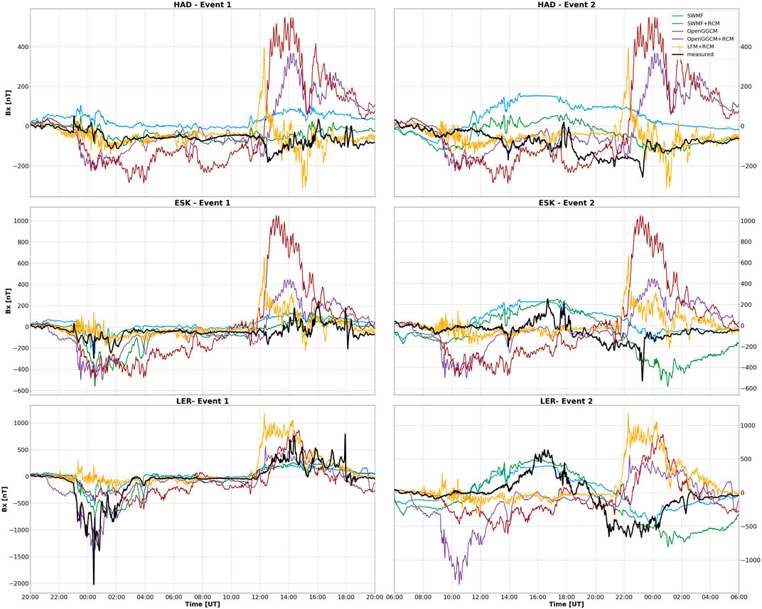
FIGURE 2. Northward ground magnetic field component (B_x) at HAD, ESK, LER during 7–8 September 2017 (event 1, left), and 17–18 March 2015 (event 2, right). Black line is the measured observatory values; coloured lines correspond to respective CCMC models.

FIGURE 3

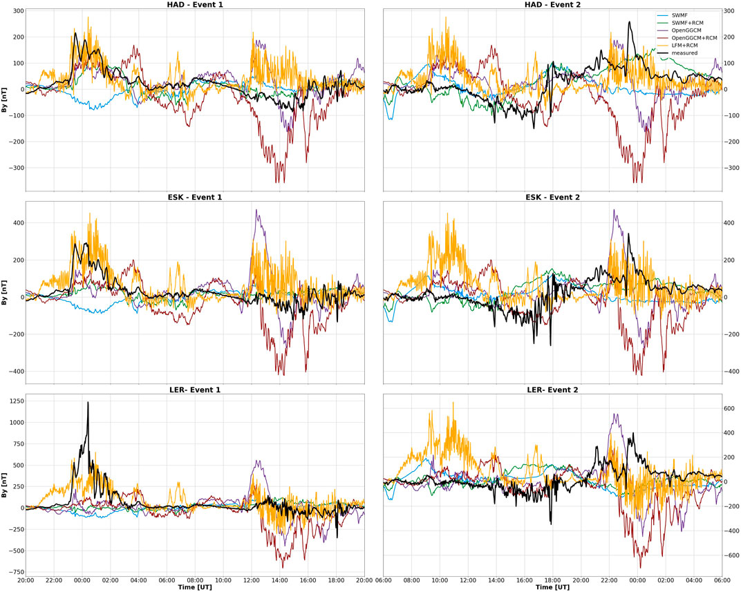
FIGURE 3. Eastward ground magnetic field component (B_y) at HAD, ESK, LER during 7–8 September 2017 (event 1, left), and 17–18 March 2015 (event 2, right). Black line is the measured observatory values; coloured lines correspond to respective CCMC models.

4.1 nRMSE and correlation

Figure 4 and Figure 5 show the normalised root-mean-square errors (top) and Pearson’s correlation coefficients (bottom) for B_x and B_y components, respectively. In terms of the B_x, similar trends can be seen during both events (Figure 4). The mean (pink line) and median (navy line) metrics are also plotted to show the average performance of all models per observatory as well as their accuracy after removing the extreme values. Those results indicate that the overall performance of all models tends to increase with increasing latitude, where nRMSE and correlation coefficients reach values closer to one in most cases. The accuracy of respective simulations in predicting B_x vary between observatories. The SWMF and SWMF + RCM perform relatively well in terms of both the overall nRMSE and correlation values for both events. The OpenGGCM model shows similar patterns but with higher nRMSE and lower correlation in comparison to the SWMF results, particularly in terms of event 2. The addition of RCM makes the OpenGGCM the least accurate simulation during the two events investigated. The LFM + RCM shows about average performance at all three observatories, with rather poor correlation with measurements, especially during the March 2015 (event 2).

FIGURE 4

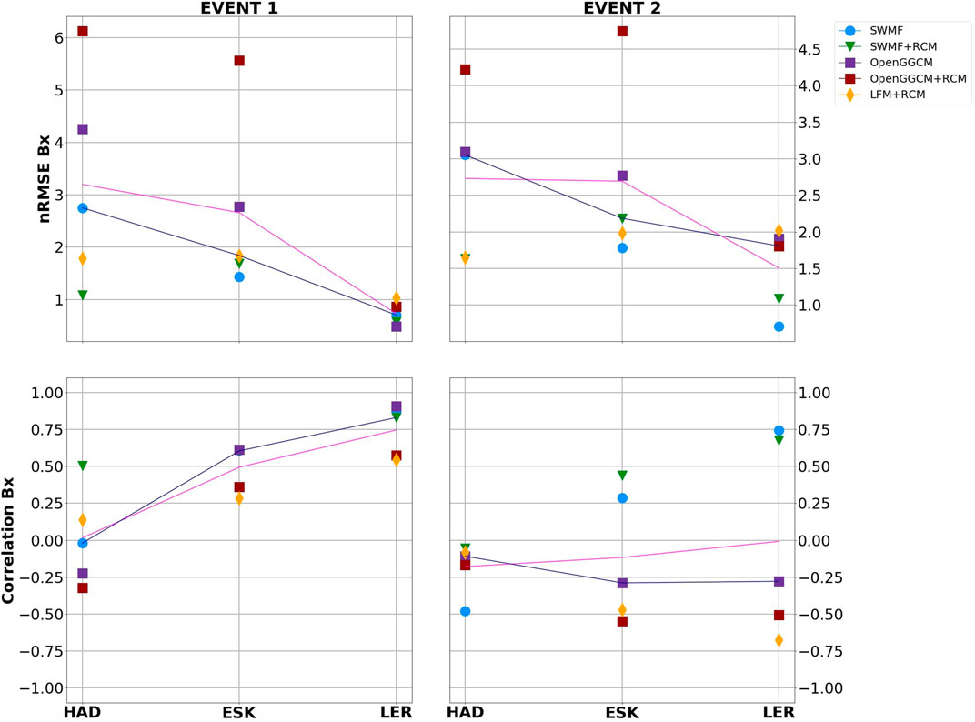
FIGURE 4. Normalised root-mean-squared errors (nRMSE) (top) and Pearson’s correlation coefficients (bottom) for B_x at each station and both events. Pink and navy lines indicate the mean and median metric value per observatory of all models, respectively. Latitude increases from left to right.

FIGURE 5

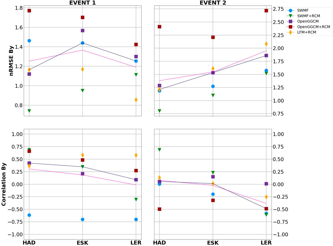
FIGURE 5. Normalised root-mean-squared errors (nRMSE) (top) and Pearson’s correlation coefficients (bottom) for B_y at each station and both events. Pink and navy lines indicate the mean and median metric value per observatory, respectively. Latitude increases from left to right.

There is no distinct pattern in the simulation performance when predicting the B_y component (Figure 5). The mean and median values show an increase in overall model error at ESK for event 1, and tend to increase with latitude for event 2, the opposite of what was observed for B_x. Correlation coefficients for both events gradually decrease at higher latitudes. In this case, significant differences between SWMF and SWMF coupled with RCM can be seen, though the addition of RCM improves the model performance during both events. However, the SWMF gives overall poor results, especially for the September 2017 event. The OpenGGCM gives similar error values for all latitudes and events, with the exception of ESK for event 1. The resulting correlation coefficients also remain the same, fluctuating between 0 and 0.45, which indicates relatively little correlation. As seen in B_x, the OpenGGCM + RCM ground magnetic field predictions result in large values of nRMSE for both events. However, data-model correlation in this case is quite high in comparison with other models for event 1. Based on the two metrics, the LFM + RCM shows similar behaviour to the OpenGGCM simulation, staying relatively close to the mean/median values. Its performance during the September 2017 storm is one of the best amongst all simulations.

4.2 Threshold metrics

The following set of event detection metrics are based on the calculated horizontal magnetic field component (B_H). A threshold of $>$150 nT (indicating intense storm conditions) was selected for both storms for all three observatories. Figures 6, 7 show Probability of Detection (POD), Probability of False Detection (POFD), Heidke Skill Score (HSS) and Frequency Bias (FB). Similarly to nRMSE and correlation plots, the pink trace indicates the mean and the navy trace the median of all metrics at each station. The dashed lines on each plot represent 0.5 for both POD and POFD, 0 for HSS and 1 for FB. For a good model performance, the following results would be required: POD $>$ 0.5, POFD $<$ 0.5, HSS $>$ 0 and FB ≈ 1.

FIGURE 6

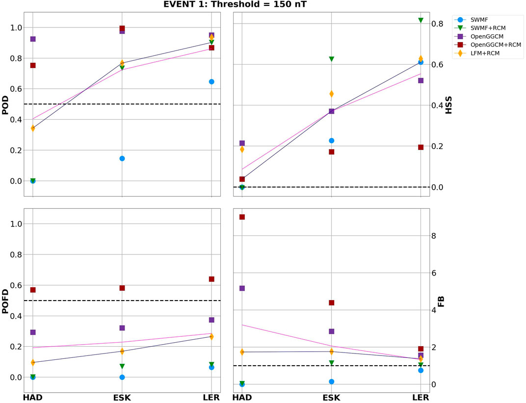
FIGURE 6. POD, POFD, HSS, and FB metrics for B_H = 150 nT threshold at each station during event 1. Pink and navy lines indicate the mean and median metric value per observatory, respectively.

During the September 2017 storm (Figure 6) a pattern can be observed in all four metrics. Mean and median POD, HSS and FB tend to have more acceptable values at higher latitudes. The resulting POFDs do not vary drastically at different stations, staying below 0.5. The SWMF horizontal field shows poor results in terms of POD, with values close to 0 at HAD and ESK, and below 0.7 at LER. The POFD gives a reasonable value at all stations. This implies that the model correctly predicts no threshold crossings but at the same time forecasts more false alarms (i.e., overpredicts). The skill score indicates rather poor model performance at lower latitudes, though reaches relatively high value at LER ($>$0.65). The FB at all latitudes remains below 1 which indicates that the model predicts events less frequently than reality. The B_H component forecast from the SWMF + RCM follows a similar pattern to the SWMF, however with much better POD and HSS results and slightly worse POFD. The SWMF + RCM also shows the best FB amongst all models, with values close to 1 at all stations, meaning that, in general, it predicts threshold crossings almost as frequently as observations. The OpenGGCM simulation performs better than SWMF in terms of POD, that is predicts more correct crossings than misses, but gives higher values of POFD. On average, the resulting skill scores remain below 0.5, indicating poor accuracy particularly at lower latitudes. The OpenGGCM seems to forecast events more often than they occur, with high values of FB. As observed with the nRMSE and correlation analysis, the addition of RCM decreases its overall predictive power. The LFM + RCM model combination results in quite high POD, low POFD and relatively good HSS and FB at all stations.

During the March 2015 storm (Figure 7) the performance of simulations varies more drastically between the observatories, particularly in terms of HSS. A similar pattern can still be observed, with better results at the highest latitude. However, in this case both POD and POFD increase with latitude, as shown by the mean and median traces. On average most models show POD $<$0.5 at HAD and POFD $>$0.5 at LER. This implies that models tend to predict just as many correct crossings as false alarms. Contrary to the September 2017 event, the skill scores do not exceed values of 0.3, indicating poor performance overall. In general, most simulations forecast threshold crossings more frequently than observations (FB $>$ 1), with HAD being the only exception. The accuracy of SWMF in terms of all 4 metrics increases with latitude, following the general trend. Here, the addition of the RCM seems to improve its performance in correct threshold crossings (higher POD) and HSS. The results provided by the OpenGGCM simulation show rather average agreement with observations overall, and quite poor skill score ($<$0) at the highest latitude. The OpenGGCM + RCM shows similar trends to those seen for the first event. Lastly, the LFM + RCM simulation during event 2 follows the average pattern in terms of POD, POFD and FB, sitting relatively close to the median line. Its skill scores vary between observatories, reaching the highest value at ESK and lowest at LER.

FIGURE 7

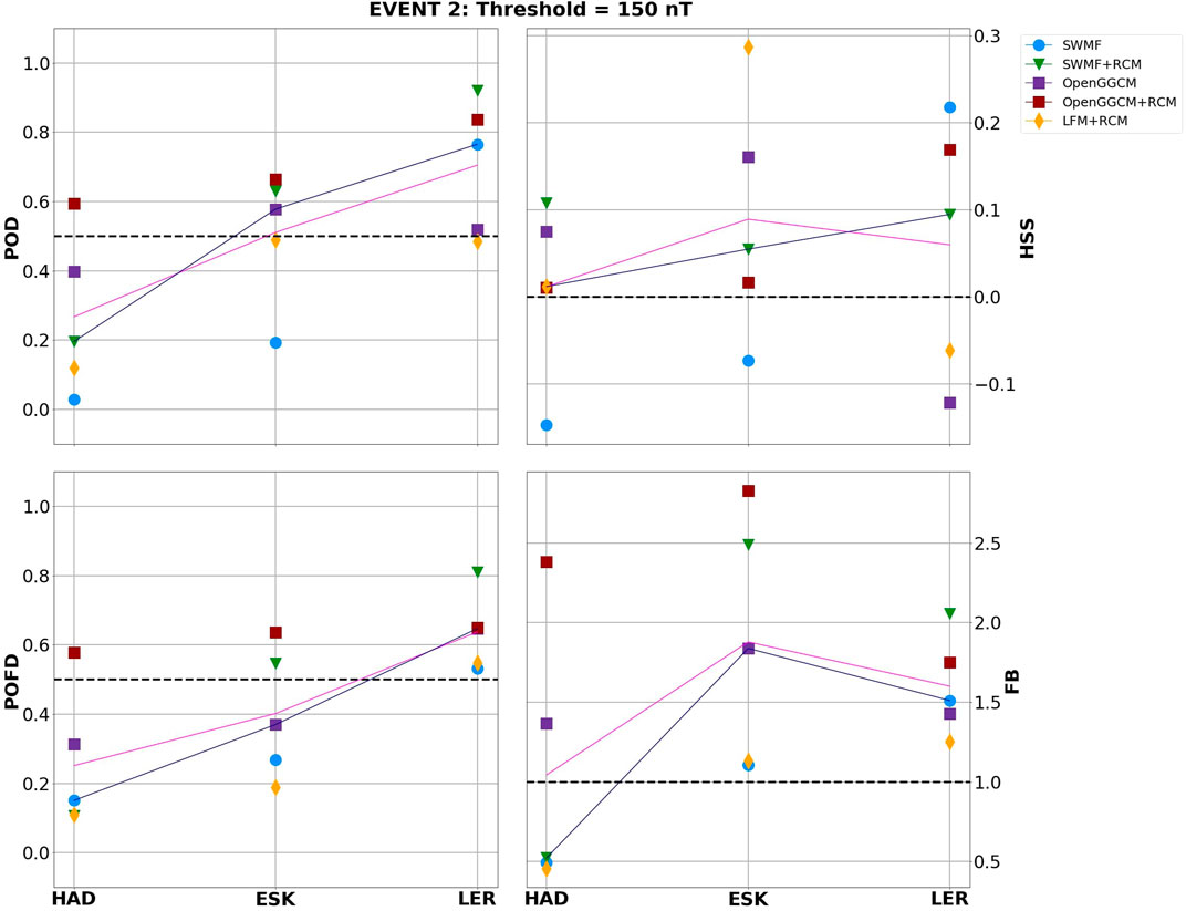
FIGURE 7. POD, POFD, HSS and FB metrics for B_H = 150 nT threshold at each station during event 2. Pink and navy lines indicate the mean and median metric value per observatory, respectively.

5 Discussion and summary

Our study investigates the performance of various contemporary global MHD models in their ability to forecast ground magnetic field perturbations during two severe geomagnetic storms in 2015 and 2017. Such MHD models are increasingly being used to provide operational services for predicting values of ground geomagnetic field and to provide hazard warnings tens of minutes in advance of an anticipated space weather event based on solar wind measurements at L1. In theory, even longer warning lead times, up to days, could be provided based on solar wind propagation of a CME from initial detection.

The simulated northward B_x, eastward B_y and the resulting horizontal B_H components were compared with ground magnetometer data from three United Kingdom observatories: Hartland, Eskdalemuir and Lerwick. In general, there is no systematic model ranking for any events or components examined and the overall performance of each simulation is highly dependent on the type of metric used in the data-model comparison, as previously seen by Pulkkinen et al. (2011). There is no preferred or “best” model. However, the following trends were observed:

• Models tend to exaggerate the magnitude of ground variations at lower latitudes but perform relatively better at higher latitudes ($>60°$N), with lowest nRMSE and highest correlation coefficients, especially during the September 2017 storm.

• Overall, all models show rather poor correlation with measured data during both storms. Correlations barely exceed 0.75 and often reach negative values.

• The B_H component analysis indicates that, on average, models predict threshold crossings more accurately during the September 2017 (event 1), where the average POD and POFD remain above and below 0.5, respectively and HSS is above 0 at all latitudes, with significant increase at LER.

• Frequency Bias values for both events suggest that all models have a tendency to predict threshold crossings (i.e. storm periods) more often than in reality but become closer to observations at higher latitudes.

• The RCM in combination with the OpenGGCM decreases the model accuracy, resulting in large overestimates of magnetic field amplitude when compared with observations.

Currently-available global MHD models of the magnetosphere and ionosphere have several limitations that affect their overall performance in the magnetic field forecast. Simplified solar wind input parameters might result in timing errors, consequently causing the model output to capture ground disturbances before or after their actual occurrence. Previous research (Freeman et al., 2019; Dimmock et al., 2021) also notes that MHD models regularly fail to represent substorm characteristics, identified as more rapid and frequent disturbances observed mainly in high-latitude and auroral regions (Daglis et al., 2003; Tanskanen et al., 2011), and large changes in the B-field amplitude associated with those events. The results presented in this study also confirm those observations. Another often seen problem with accuracy is that models occasionally predict the opposite sign of modelled ground perturbation, most likely due to a shift in location of the electrojets in the simulated magnetospheric and ionospheric currents compared to their actual location.

An accurate representation of both the amplitude and timing (i.e., phase) of directly-driven field variation during geomagnetically active times is vital for actionable space weather hazard forecasts. The results here suggest that this goal has not yet been reached and much work remains to produce a sufficiently robust estimate of ground magnetic field variations experienced at mid-latitudes. It has to be noted however that our study was limited to only two storms and three observatories for a highly localised analysis. More stations and space weather events should be included in future investigations to provide more systematic and unbiased conclusions regarding the accuracy of MHD simulations.

Data availability statement

Publicly available datasets were analyzed in this study. These data can be found here: ESK, HAD, LER magnetic field data for 17th - 18th March 2015 and 7th - 8th September 2017 can be downloaded from: https://www.intermagnet.org/data-donnee/download-eng.php#view All CCMC model runs included in analysis: Ewelina_Florczak_030821_3, Ewelina_Florczak_030821_4, Ewelina_Florczak_011222_1, Ewelina_Florczak_011222_2, Ewelina_Florczak_070222_3, Ewelina_Florczak_070222_4, Ewelina_Florczak_070222_5, Ewelina_Florczak_070222_6, Ewelina_Florczak_070222_7, Ewelina_Florczak_070222_8 are available at https://ccmc.gsfc.nasa.gov/ungrouped/search_main.php.

Author contributions

EF—collecting data, comparison and analysis, coding, paper preparation CB—research idea, coding, proof reading and review KW—research idea, proof reading and review.

Funding

This work was carried out using the SWMF and BATS-R-US tools developed at the University of Michigan’s Center for Space Environment Modeling (CSEM), the OpenGGCM developed at UCLA by Joachim Raeder, the LFM Model first introduced by John Lyon, Joel Fedder, and Clark Mobarry, as well as the Rice Convection Model developed by the Department of Physics and Astronomy at Rice University. Additional resources are provided by the OMNIWeb Plus data service at Goddard Space Flight Center.

Acknowledgments

The results presented in this paper rely on data collected at magnetic observatories: Hartland (HAD), Eskdalemuir (ESK) and Lerwick (LER). We thank the national institutes that support them and INTERMAGNET for promoting high standards of magnetic observatory practice (www.intermagnet.org). Simulation results have been provided by the Community Coordinated Modeling Center at Goddard Space Flight Center through their public Runs on Request system (http://ccmc.gsfc.nasa.gov).

Conflict of interest

The authors declare that the research was conducted in the absence of any commercial or financial relationships that could be construed as a potential conflict of interest.

Publisher’s note

All claims expressed in this article are solely those of the authors and do not necessarily represent those of their affiliated organizations, or those of the publisher, the editors and the reviewers. Any product that may be evaluated in this article, or claim that may be made by its manufacturer, is not guaranteed or endorsed by the publisher.

Footnotes

¹https://wdc.kugi.kyoto-u.ac.jp/.

²https://www.intermagnet.org/data-donnee/download-eng.php.

³https://ccmc.gsfc.nasa.gov/tools/runs-on-request/.

References

Bartels, J., Heck, N., and Johnston, H. (1939). The three-hour-range index measuring geomagnetic activity. Terr. Magnetism Atmos. Electr. 44, 411–454. doi:10.1029/te044i004p00411

CrossRef Full Text | Google Scholar

Beggan, C. D., Richardson, G. S., Baillie, O., Hübert, J., and Thomson, A. W. (2021). Geolectric field measurement, modelling and validation during geomagnetic storms in the UK. J. space weather space Clim. 11, 37. doi:10.1051/swsc/2021022

CrossRef Full Text | Google Scholar

Bolduc, L. (2002). GIC observations and studies in the Hydro-Québec power system. J. Atmos. Solar-Terrestrial Phys. 64, 1793–1802. doi:10.1016/s1364-6826(02)00128-1

CrossRef Full Text | Google Scholar

Bolduc, L., Langlois, P., Boteler, D., and Pirjola, R. (1998). A study of geoelectromagnetic disturbances in Quebec. I. General results. IEEE Trans. Power Deliv. 13, 1251–1256. doi:10.1109/61.714492

CrossRef Full Text | Google Scholar

Boteler, D. (2019). A 21st century view of the march 1989 magnetic storm. Space weather. 17, 1427–1441. doi:10.1029/2019sw002278

CrossRef Full Text | Google Scholar

Boteler, D. (1994). Geomagnetically induced currents: Present knowledge and future research. IEEE Trans. Power Deliv. 9, 50–58. doi:10.1109/61.277679

CrossRef Full Text | Google Scholar

Boteler, D. (2021). Modeling geomagnetic interference on railway signaling track circuits. Space weather. 19, e2020SW002609. doi:10.1029/2020sw002609

CrossRef Full Text | Google Scholar

Boteler, D., Pirjola, R., and Nevanlinna, H. (1998). The effects of geomagnetic disturbances on electrical systems at the Earth’s surface. Adv. Space Res. 22, 17–27. doi:10.1016/s0273-1177(97)01096-x

CrossRef Full Text | Google Scholar

Carter, B., Yizengaw, E., Pradipta, R., Weygand, J., Piersanti, M., Pulkkinen, A., et al. (2016). Geomagnetically induced currents around the world during the 17 March 2015 storm. J. Geophys. Res. Space Phys. 121, 10–496. doi:10.1002/2016ja023344

CrossRef Full Text | Google Scholar

Chapman, S. C., Horne, R. B., and Watkins, N. W. (2020). Using the aa index over the last 14 solar cycles to characterize extreme geomagnetic activity. Geophys. Res. Lett. 47, e2019GL086524. doi:10.1029/2019GL086524

CrossRef Full Text | Google Scholar

Clilverd, M. A., Rodger, C. J., Brundell, J. B., Dalzell, M., Martin, I., Mac Manus, D. H., et al. (2018). Long-lasting geomagnetically induced currents and harmonic distortion observed in New Zealand during the 7–8 September 2017 disturbed period. Space weather. 16, 704–717. doi:10.1029/2018sw001822

CrossRef Full Text | Google Scholar

Cliver, E. W., and Dietrich, W. F. (2013). The 1859 space weather event revisited: Limits of extreme activity. J. Space Weather Space Clim. 3, A31. doi:10.1051/swsc/2013053

CrossRef Full Text | Google Scholar

Cramer, W. D., Raeder, J., Toffoletto, F., Gilson, M., and Hu, B. (2017). Plasma sheet injections into the inner magnetosphere: Two-way coupled OpenGGCM-RCM model results. J. Geophys. Res. Space Phys. 122, 5077–5091. doi:10.1002/2017ja024104

CrossRef Full Text | Google Scholar

Daglis, I., Kozyra, J., Kamide, Y., Vassiliadis, D., Sharma, A., Liemohn, M., et al. (2003). Intense space storms: Critical issues and open disputes. J. Geophys. Res. Space Phys. 108. doi:10.1029/2002ja009722

CrossRef Full Text | Google Scholar

Dang, T., Li, X., Luo, B., Li, R., Zhang, B., Pham, K., et al. (2022). Unveiling the space weather during the starlink satellites destruction event on 4 february 2022. Space weather. 20, e2022SW003152. doi:10.1029/2022sw003152

CrossRef Full Text | Google Scholar

Dimmock, A. P., Rosenqvist, L., Hall, J.-O., Viljanen, A., Yordanova, E., Honkonen, I., et al. (2019). The GIC and geomagnetic response over Fennoscandia to the 7–8 September 2017 geomagnetic storm. Space weather. 17, 2018SW002132–1010. doi:10.1029/2018sw002132

CrossRef Full Text | Google Scholar

Dimmock, A., Welling, D., Rosenqvist, L., Forsyth, C., Freeman, M., Rae, I., et al. (2021). Modeling the geomagnetic response to the September 2017 space weather event over Fennoscandia using the Space Weather Modeling Framework: Studying the impacts of spatial resolution. Space weather. 19, e2020SW002683. doi:10.1029/2020sw002683

CrossRef Full Text | Google Scholar

Divett, T., Richardson, G., Beggan, C., Rodger, C., Boteler, D., Ingham, M., et al. (2018). Transformer-level modeling of geomagnetically induced currents in New Zealand’s South Island. Space weather. 16, 718–735. doi:10.1029/2018sw001814

CrossRef Full Text | Google Scholar

Feng, X., and Feng, X. (2020). Current status of mhd simulations for space weather. Magnetohydrodynamic Model. Sol. Corona Heliosphere 2020, 1–123. doi:10.1007/978-981-13-9081-4_1

CrossRef Full Text | Google Scholar

Freeman, M. P., Forsyth, C., and Rae, I. J. (2019). The influence of substorms on extreme rates of change of the surface horizontal magnetic field in the United Kingdom. Space weather. 17, 827–844. doi:10.1029/2018sw002148

CrossRef Full Text | Google Scholar

Fuller-Rowell, T., Rees, D., Quegan, S., Moffett, R., Codrescu, M., and Millward, G. (1996). A coupled thermosphere-ionosphere model (CTIM). STEP Rep. 239.

Google Scholar

Glocer, A., Fok, M., Meng, X., Toth, G., Buzulukova, N., Chen, S., et al. (2013). CRCM+BATS–R–US two–way coupling. J. Geophys. Res. Space Phys. 118, 1635–1650. doi:10.1002/jgra.50221

CrossRef Full Text | Google Scholar

Glocer, A., Tóth, G., Ma, Y., Gombosi, T., Zhang, J.-C., and Kistler, L. (2009). Multifluid block-adaptive-tree solar wind roe-type upwind scheme: Magnetospheric composition and dynamics during geomagnetic storms—Initial results. J. Geophys. Res. Space Phys. 114, 1. doi:10.1029/2009ja014418

CrossRef Full Text | Google Scholar

Gombosi, T. I., Tóth, G., Zeeuw, D., Hansen, K. C., Kabin, K., and Powell, K. G. (2002). Semirelativistic magnetohydrodynamics and physics-based convergence acceleration. J. Comput. Phys. 177, 176–205. doi:10.1006/jcph.2002.7009

CrossRef Full Text | Google Scholar

Goodrich, C., Sussman, A., Lyon, J., Shay, M., and Cassak, P. (2004). The CISM code coupling strategy. J. Atmos. solar-terrestrial Phys. 66, 1469–1479. doi:10.1016/j.jastp.2004.04.010

CrossRef Full Text | Google Scholar

Guerrero, A., Palacios, J., Rodríguez-Bouza, M., Rodríguez-Bilbao, I., Aran, A., Cid, C., et al. (2017). Storm and substorm causes and effects at midlatitude location for the St. Patrick’s 2013 and 2015 events. J. Geophys. Res. Space Phys. 122, 9994–10,011. doi:10.1002/2017ja024224

CrossRef Full Text | Google Scholar

Hayakawa, H., Ebihara, Y., Willis, D. M., Toriumi, S., Iju, T., Hattori, K., et al. (2019). Temporal and spatial evolutions of a large sunspot group and great auroral storms around the Carrington event in 1859. Space weather. 17, 1553–1569. doi:10.1029/2019sw002269

CrossRef Full Text | Google Scholar

Hénon, M. (1982). Vlasov equation. Astronomy Astrophysics 114, 211.

Google Scholar

Hogan, R., and Mason, I. (2012). Deterministic forecasts of binary events. Hoboken: Wiley.

Google Scholar

Huba, J., Sazykin, S., and Coster, A. (2017). Sami3-RCM simulation of the 17 March 2015 geomagnetic storm. J. Geophys. Res. Space Phys. 122, 1246–1257. doi:10.1002/2016ja023341

CrossRef Full Text | Google Scholar

Kelly, G., Viljanen, A., Beggan, C., and Thomson, A. (2017). Understanding gic in the UK and French high-voltage transmission systems during severe magnetic storms. Space weather. 15, 99–114. doi:10.1002/2016sw001469

CrossRef Full Text | Google Scholar

Kwagala, N. K., Hesse, M., Moretto, T., Tenfjord, P., Norgren, C., Tóth, G., et al. (2020). Validating the space weather modeling framework (SWMF) for applications in northern europe - ground magnetic perturbation validation. J. Space Weather Space Clim. 10, 33. doi:10.1051/swsc/2020034

CrossRef Full Text | Google Scholar

Liemohn, M. W., Shane, A. D., Azari, A. R., Petersen, A. K., Swiger, B. M., and Mukhopadhyay, A. (2021). Rmse is not enough: Guidelines to robust data-model comparisons for magnetospheric physics. J. Atmos. Solar-Terrestrial Phys. 218, 105624. doi:10.1016/j.jastp.2021.105624

CrossRef Full Text | Google Scholar

Lyon, J., Fedder, J., and Mobarry, C. (2004). The Lyon–Fedder–Mobarry (LFM) global MHD magnetospheric simulation code. J. Atmos. Solar-Terrestrial Phys. 66, 1333–1350. doi:10.1016/j.jastp.2004.03.020

CrossRef Full Text | Google Scholar

Merkin, V., and Lyon, J. (2010). Effects of the low-latitude ionospheric boundary condition on the global magnetosphere. J. Geophys. Res. Space Phys. 115, 11. doi:10.1029/2010ja015461

CrossRef Full Text | Google Scholar

Ngwira, C. M., Sibeck, D., Silveira, M. V., Georgiou, M., Weygand, J. M., Nishimura, Y., et al. (2018). A study of intense local dB/dt variations during two geomagnetic storms. Space weather. 16, 676–693. doi:10.1029/2018sw001911

CrossRef Full Text | Google Scholar

Oughton, E. J., Hapgood, M., Richardson, G. S., Beggan, C. D., Thomson, A. W., Gibbs, M., et al. (2019). A risk assessment framework for the socioeconomic impacts of electricity transmission infrastructure failure due to space weather: An application to the United Kingdom. Risk Anal. 39, 1022–1043. doi:10.1111/risa.13229

PubMed Abstract | CrossRef Full Text | Google Scholar

Piersanti, M., Di Matteo, S., Carter, B., Currie, J., and D’Angelo, G. (2019). Geoelectric field evaluation during the september 2017 geomagnetic storm: MA. I. GIC. Model. Space weather. 17, 1241–1256. doi:10.1029/2019sw002202

CrossRef Full Text | Google Scholar

Pirjola, R. (2000). Geomagnetically induced currents during magnetic storms. IEEE Trans. plasma Sci. 28, 1867–1873. doi:10.1109/27.902215

CrossRef Full Text | Google Scholar

Powell, K. G., Roe, P. L., Linde, T. J., Gombosi, T. I., and Zeeuw, D., (1999). A solution-adaptive upwind scheme for ideal magnetohydrodynamics. J. Comput. Phys. 154, 284–309. doi:10.1006/jcph.1999.6299

CrossRef Full Text | Google Scholar

Pulkkinen, A., Kuznetsova, M., Ridley, A., Raeder, J., Vapirev, A., Weimer, D., et al. (2011). Geospace environment modeling 2008–2009 challenge: Ground magnetic field perturbations. Space weather. 9. doi:10.1029/2010sw000600

CrossRef Full Text | Google Scholar

Pulkkinen, A., Rastätter, L., Kuznetsova, M., Singer, H., Balch, C., Weimer, D., et al. (2013). Community-wide validation of geospace model ground magnetic field perturbation predictions to support model transition to operations. Space weather. 11, 369–385. doi:10.1002/swe.20056

CrossRef Full Text | Google Scholar

Qian, L., Wang, W., Burns, A. G., Chamberlin, P. C., Coster, A., Zhang, S.-R., et al. (2019). Solar flare and geomagnetic storm effects on the thermosphere and ionosphere during 6–11 September 2017. J. Geophys. Res. Space Phys. 124, 2298–2311. doi:10.1029/2018ja026175

CrossRef Full Text | Google Scholar

Raeder, J., Cramer, W., Germaschewski, K., and Jensen, J. (2017). Using OpenGGCM to compute and separate magnetosphere magnetic perturbations measured on board low earth orbiting satellites. Space Sci. Rev. 206, 601–620. doi:10.1007/s11214-016-0304-x

CrossRef Full Text | Google Scholar

Raeder, J., Larson, D., Li, W., Kepko, E. L., and Fuller-Rowell, T. (2008). OpenGGCM simulations for the THEMIS mission. Space Sci. Rev. 141, 535–555. doi:10.1007/s11214-008-9421-5

CrossRef Full Text | Google Scholar

Rajput, V. N., Boteler, D. H., Rana, N., Saiyed, M., Anjana, S., and Shah, M. (2021). Insight into impact of geomagnetically induced currents on power systems: Overview, challenges and mitigation. Electr. Power Syst. Res. 192, 106927. doi:10.1016/j.epsr.2020.106927

CrossRef Full Text | Google Scholar

Rastätter, L., Kuznetsova, M., Glocer, A., Welling, D., Meng, X., Raeder, J., et al. (2013). Geospace environment modeling 2008–2009 challenge: Dst index. Space weather. 11, 187–205. doi:10.1002/swe.20036

CrossRef Full Text | Google Scholar

Rastätter, L., Kuznetsova, M., Vapirev, A., Ridley, A., Wiltberger, M., Pulkkinen, A., et al. (2011). Geospace environment modeling 2008–2009 challenge: Geosynchronous magnetic field. Space Weather Int. J. Res. Appl. 9, 4. doi:10.1029/2010SW000617,

CrossRef Full Text | Google Scholar

Rastätter, L., Tóth, G., Kuznetsova, M. M., and Pulkkinen, A. A. (2014). CalcDeltaB: An efficient postprocessing tool to calculate ground-level magnetic perturbations from global magnetosphere simulations. Space weather. 12, 553–565. doi:10.1002/2014sw001083

CrossRef Full Text | Google Scholar

Reay, S., Allen, W., Baillie, O., Bowe, J., Clarke, E., Lesur, V., et al. (2005). Space weather effects on drilling accuracy in the North Sea. Ann. Geophys. Copernic. GmbH) 23, 3081–3088. doi:10.5194/angeo-23-3081-2005

CrossRef Full Text | Google Scholar

Richmond, A., Ridley, E., and Roble, R. (1992). A thermosphere/ionosphere general circulation model with coupled electrodynamics. Geophys. Res. Lett. 19, 601–604. doi:10.1029/92gl00401

CrossRef Full Text | Google Scholar

Ridley, A., De Zeeuw, D., and Rastätter, L. (2016). Rating global magnetosphere model simulations through statistical data-model comparisons. Space weather. 14, 819–834. doi:10.1002/2016sw001465

CrossRef Full Text | Google Scholar

Rodger, C. J., Clilverd, M. A., Manus, M, Martin, I., Dalzell, M., Brundell, J. B., et al. (2020). Geomagnetically induced currents and harmonic distortion: Storm-time observations from New Zealand. Space weather. 18, e2019SW002387. doi:10.1029/2019sw002387

CrossRef Full Text | Google Scholar

Sazykin, S., Wolf, R., Spiro, R., Gombosi, T., De Zeeuw, D., and Thomsen, M. (2002). Interchange instability in the inner magnetosphere associated with geosynchronous particle flux decreases. Geophys. Res. Lett. 29, 88. doi:10.1029/2001gl014416

CrossRef Full Text | Google Scholar

Simpson, F., and Bahr, K. (2021). Nowcasting and validating Earth’s electric field response to extreme space weather events using magnetotelluric data: Application to the September 2017 geomagnetic storm and comparison to observed and modeled fields in Scotland. Space weather. 19, e2019SW002432. doi:10.1029/2019sw002432

CrossRef Full Text | Google Scholar

Smith, A., Forsyth, C., Rae, I., Garton, T., Bloch, T., Jackman, C., et al. (2021). Forecasting the probability of large rates of change of the geomagnetic field in the UK: Timescales, horizons, and thresholds. Space weather. 19, e2021SW002788. doi:10.1029/2021sw002788

CrossRef Full Text | Google Scholar

Stout, Q. F., Zeeuw, De, Gombosi, T. I., Groth, C. P., Marshall, H. G., and Powell, K. G. (1997). “Adaptive blocks: A high performance data structure,” in Proceedings of the 1997 ACM/IEEE conference on Supercomputing, New York, 15 November 1997 (IEEE), 1.

Google Scholar

Tanskanen, E., Pulkkinen, T. I., Viljanen, A., Mursula, K., Partamies, N., and Slavin, J. (2011). From space weather toward space climate time scales: Substorm analysis from 1993 to 2008. J. Geophys. Res. Space Phys. 116, 1. doi:10.1029/2010ja015788

CrossRef Full Text | Google Scholar

Toffoletto, F., Sazykin, S., Spiro, R., and Wolf, R. (2003). Inner magnetospheric modeling with the Rice convection model. Space Sci. Rev. 107, 175–196. doi:10.1023/a:1025532008047

CrossRef Full Text | Google Scholar

Tóth, G., Sokolov, I. V., Gombosi, T. I., Chesney, D. R., Clauer, C. R., De Zeeuw, D. L., et al. (2005). Space weather modeling framework: A new tool for the space science community. J. Geophys. Res. Space Phys. 110, A12226. doi:10.1029/2005ja011126

CrossRef Full Text | Google Scholar

Viljanen, A., Nevanlinna, H., Pajunpää, K., and Pulkkinen, A. (2001). Time derivative of the horizontal geomagnetic field as an activity indicator. Ann. Geophys. Copernic. GmbH) 19, 1107–1118. doi:10.5194/angeo-19-1107-2001

CrossRef Full Text | Google Scholar

Wang, W., Wiltberger, M., Burns, A., Solomon, S., Killeen, T., Maruyama, N., et al. (2004). Initial results from the coupled magnetosphere–ionosphere–thermosphere model: Thermosphere–ionosphere responses. J. Atmos. solar-terrestrial Phys. 66, 1425–1441. doi:10.1016/j.jastp.2004.04.008

CrossRef Full Text | Google Scholar

Wanliss, J. A., and Showalter, K. M. (2006). High-resolution global storm index: Dst versus sym-h. J. Geophys. Res. Space Phys. 111, A02202. doi:10.1029/2005ja011034

CrossRef Full Text | Google Scholar

Welling, D. T., Anderson, B. J., Crowley, G., Pulkkinen, A. A., and Rastätter, L. (2017). Exploring predictive performance: A reanalysis of the geospace model transition challenge. Space weather. 15, 192–203. doi:10.1002/2016sw001505

CrossRef Full Text | Google Scholar

Wiltberger, M., Wang, W., Burns, A., Solomon, S., Lyon, J., and Goodrich, C. (2004). Initial results from the coupled magnetosphere ionosphere thermosphere model: Magnetospheric and ionospheric responses. J. Atmos. solar-terrestrial Phys. 66, 1411–1423. doi:10.1016/j.jastp.2004.03.026

CrossRef Full Text | Google Scholar

Wolf, R., Harel, M., Spiro, R., Voigt, G.-H., Reiff, P., and Chen, C.-K. (1977). Computer simulation of inner magnetospheric dynamics for the magnetic storm of. J. Geophys. Res. Space Phys. 87, 5949–5962. doi:10.1029/JA087iA08p05949

CrossRef Full Text | Google Scholar

Wolf, R., Spiro, R., Sazykin, S., and Toffoletto, F. (2007). How the Earth’s inner magnetosphere works: An evolving picture. J. Atmos. Solar-Terrestrial Phys. 69, 288–302. doi:10.1016/j.jastp.2006.07.026

CrossRef Full Text | Google Scholar

Yu, Y., and Ridley, A. J. (2008). Validation of the space weather modeling framework using ground-based magnetometers. Space weather. 6. doi:10.1029/2007sw000345

CrossRef Full Text | Google Scholar

Zaharia, S., Jordanova, V., Welling, D., and Tóth, G. (2010). Self-consistent inner magnetosphere simulation driven by a global MHD model. J. Geophys. Res. Space Phys. 115, 1. doi:10.1029/2010ja015915

CrossRef Full Text | Google Scholar

Zeeuw, D, Gombosi, T. I., Groth, C. P., Powell, K. G., and Stout, Q. F. (2000). An adaptive MHD method for global space weather simulations. IEEE Trans. Plasma Sci. 28, 1956–1965. doi:10.1109/27.902224

CrossRef Full Text | Google Scholar

Zeeuw, D, Sazykin, S., Wolf, R. A., Gombosi, T. I., Ridley, A. J., and Tóth, G. (2004). Coupling of a global MHD code and an inner magnetospheric model: Initial results. J. Geophys. Res. Space Phys. 109, A12219. doi:10.1029/2003ja010366

CrossRef Full Text | Google Scholar

Zhang, J., Liemohn, M. W., Zeeuw, De, Borovsky, J. E., Ridley, A. J., Toth, G., et al. (2007). Understanding storm-time ring current development through data-model comparisons of a moderate storm. J. Geophys. Res. Space Phys. 112, 12. doi:10.1029/2006ja011846

CrossRef Full Text | Google Scholar

Zhang, J., Wang, C., Sun, T., Liu, C., and Wang, K. (2015). Gic due to storm sudden commencement in low-latitude high-voltage power network in China: Observation and simulation. Space weather. 13, 643–655. doi:10.1002/2015sw001263

CrossRef Full Text | Google Scholar

Zhang, J., Wang, C., Sun, T., and Liu, Y. D. (2016). Risk assessment of the extreme interplanetary shock of 23 july 2012 on low-latitude power networks. Space weather. 14, 259–270. doi:10.1002/2015sw001347

CrossRef Full Text | Google Scholar