Evolution of coronal magnetic field parameters during X5.4 solar flare

1 Introduction

Solar flares - intense bursts of radiation due to the release and conversion of free magnetic energy stored in the complex magnetic field over active regions (ARs) on the Sun’s surface—can cause severe satellite communication (SATCOM) degradation through Sudden Ionospheric Disturbances (SIDs) (Davies, 1990). Additionally, solar energetic particles (SEPs) accelerated by flares can cause technological impacts on electronic devices on satellites, aircraft, and even on the surface of the Earth. Furthermore, the accelerated SEPs can cause biological effects on astronauts and aircrew if exceptionally energetic (Eastwood et al., 2017). Precise forecasting of solar flares can help mitigate these impacts, but unfortunately flares remain a challenge to accurately predict. Contrary to terrestrial weather forecasting, where the physical principles/processes are well understood and climatology is used supplementary to the numerical weather prediction (NWP) models that are rooted in the physics (Pu and Kalnay, 2018), operational space weather forecasting (and flare forecasting in particular) relies heavily on climatological patterns due to a limited understanding of the underlying physical processes. McIntosh (1990) created probabilistic forecasts for flares by applying Poisson statistics to observations of flare production rates for different classes of active regions. Forecasts published today from the Space Weather Prediction Center (SWPC) still follow this approach as a basis, but utilizing a blend of statistical norms (Leka et al., 2018). Two flare forecasting workshops - Barnes et al. (2016) and Leka et al. (2019) - showed that (1) no single forecasting method clearly outperformed all others, and (2) no method was substantially better than climatological forecasts. Specifically, Leka et al. (2019) found that none of the 19 flare forecasting methods that were tested worked “extraordinarily well” with no method scoring above 0.5—i.e., halfway between “no skill” and “perfect”—across all evaluation metrics utilized, and no methods scoring above 0.5 for a number of metrics.

To improve solar flare modeling and forecasting capability requires further understanding of how the Sun’s magnetic field—particularly over ARs—evolves during solar flare events and the underlying physical processes that lead to the eruption. Numerous studies have investigated the temporal evolution of various photospheric magnetic field parameters during solar eruptive phenomena, and the correlation between those parameters and flare characteristics, especially flare occurrence (e.g., Leka and Barnes, 2003; Leka and Barnes, 2007; Mason and Hoeksema, 2010; Kazachenko et al., 2017; Whitney Aegerter et al., 2020; Garland et al., 2022; Kazachenko et al., 2022). The studies referenced are by no means a full list of those performed in this area of research, but they provide a good sample of the results regarding relationships between various photospheric magnetic field parameters and solar flare occurrence. While insights on the magnetic conditions leading up to and during solar flares have been gleaned from these findings, a discriminating signature or clear predictor of solar flare occurrence within the magnetic field data has yet to be discovered. A limitation of all these studies is the use of photospheric magnetic field data considering the eruption of a flare takes place higher in the solar atmosphere in the corona. If such a signature exists, it is likely contained within coronal magnetic field data, and despite the photospheric magnetic field being the footprints of the coronal field and photospheric motions driving the twisting/shearing of coronal structures, the coronal signature is subdued or lost at the lower altitude. Parameters calculated from the 2D imprint of an intrinsically 3D coronal field will underestimate vital aspects of the field that contribute to the flaring process (Gupta et al., 2021).

Unfortunately, the full vector-field component data available for the photosphere, is not available for the corona. However, the coronal magnetic field can be modeled. With advances in modeling of coronal fields—particularly for the field over ARs—an increasing number of studies have investigated the relationships between magnetic field parameters and flare characteristics/occurrence, as extensively examined for the photosphere, only now utilizing the modeled corona data. Inoue et al. (2011) modeled the coronal magnetic field over the flaring National Oceanic and Atmospheric Administration (NOAA) AR 10930 through Non-Linear Force-Free Field (NLFFF) extrapolation of vector magnetograms. The time series of the connectivity and twist of magnetic field lines was investigated, noting that the left-handed twist increased before the onset of the flare and quickly decreased after, consistent with the store-and-release scenario of magnetic helicity. Additionally, the analysis suggests that magnetic reconnection in a flare may commence from a region located below the most strongly twisted field. Using a sample of ten ARs, Gupta et al. (2021) performed a detailed analysis of the time evolution of the coronal magnetic energy and helicity around the time of large flares, classified as GOES class ≥ M1. The coronal field was modeled using NLFFF extrapolation, and the analysis showed that total energy and helicity budgets of flare producing ARs—i.e., extensive quantities—are not discriminative regarding the eruptive potential; however, the energy ratio, helicity ratio, and normalized current-carrying helicity—i.e. intensive quantities—seem to be distinctly different for eruptive flares compared to confined flares; Yurchyshyn et al. (2022) used Solar Dynamics Observatory (SDO) Helioseismic and Magnetic Imager (HMI) (Couvidat et al., 2016) magnetograms to perform NLFFF extrapolation of coronal magnetic field above NOAA AR 11944 in order to study the evolution of the AR’s magnetic field prior to the eruption of a X1.2 solar flare. Signatures of magnetic flux ropes (MFR) were detected at the eruption site several hour before the start of the event. The eruption site was located under a slanted sunspot field, which acted as a slanted boundary for the erupting fields to slide along as opposed to erupting vertically. Jing et al. (2018) performed a statistical analysis of torus and kink instabilities in solar eruptions. Torus instability (TI) occurs when the strapping field above an MFR decreases with height at a steep rate; kink instability (KI) occurs when an MFR is twisted beyond a critical value (Jing et al., 2018). The decay index of the potential strapping field above the MFR around the flaring magnetic primary inversion line (PIL) (TI parameter) and the unsigned twist number of the NLFFF lines forming the same MFR (KI parameter) were calculated for each event. The constructed TI-KI diagram showed that a specific threshold for the decay index discriminated between confined and ejective events, whereas the twist number does little in discriminating.

These studies (and more) demonstrate that models of the coronal magnetic field over an AR have a potential for predicting likelihood, location, and timing of solar flares. In fact, Kusano et al. (2020) developed a physics-based method, called the κ-scheme, based on the theory of double-arc instability (DAI) and utilizing NLFFF extrapolation. The κ-scheme measures the critical size of the trigger-reconnection from the vector magnetic field data on the photosphere, as well as estimates the amount of magnetic energy which is available for release by the DAI. The parameter κ is a measure of the instability (Kusano et al., 2020). Analysis of X-class flares from 2008 to 2019 showed that the scheme predicts most large, imminent flares, as well as the location they will emerge. Furthermore, the parameter of magnetic twist flux density near the PIL determines when and where solar flares may occur and how large they can be.

The purpose of this study is to investigate the evolution of the modeled coronal magnetic field data for a X5.4 solar flare event that occurred on 7 March 2012. Specifically, seven magnetic field parameters are calculated from the coronal magnetic field modeled using the same extrapolation technique as Yurchyshyn et al. (2022) for a time interval of 1 h before through 1 h after flare occurrence. The temporal evolution of the coronal magnetic field parameters leading up to and following the eruptive event was analyzed, with the ultimate intent of discerning any possible discriminating signatures or clear predictors of solar flare occurrence. Section 2 provides background information on the corona model utilized in this study; Section 3 details the methodology for extrapolating the coronal magnetic field and calculating the field parameters; Section 4 presents the preliminary results of this case study; and Section 5 summarizes the analysis and discusses future work.

2 Background

2.1 Coronal models

As mentioned previously, the efficacy of photospheric magnetic field observations in studies looking for pre-eruptive signatures of solar flare occurrence is limited due to the fact that the eruption occurs higher in the solar atmosphere in the corona. Though vector magnetic field observations are not available for the corona as they are for the photosphere, modeling of the coronal magnetic field provides an effective approach to study the state of the field during solar flare events and potentially find such signatures. Coronal magnetic field models use the photospheric magnetic field measurements as a boundary condition to model the corona. The four main types of coronal models are the Magnetohydrodynamics (MHD) model, the Magnetohydrostatic (MHS) model, the Force-Free models, and the Potential-Field Source-Surface (PFSS) model. Table 1 lists these models in order of most to least complex, as well as some of the key physical effects neglected. In the present study, the coronal magnetic field was modeled using NLFFF extrapolation; thus, the focus of this section will be on Force-Free modeling.

TABLE 1

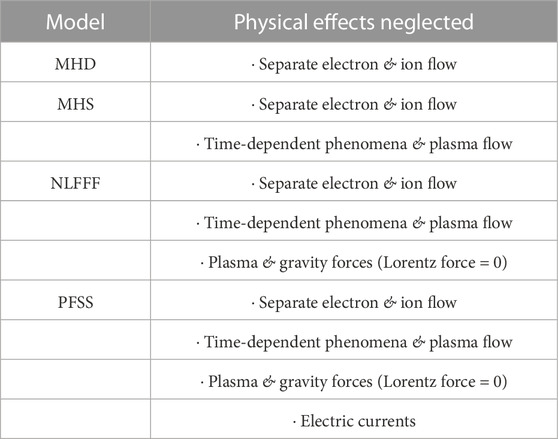
TABLE 1. A list of coronal model types.

2.1.1 Force-free field Model/NLFFF extrapolation

Unlike in the photosphere where the dense plasma dominates dynamics and the heliosphere where the solar wind is dominant, within the bulk of the corona the magnetic field dominates the plasma. From the chromosphere to about 100 Mm, where the plasma beta (β) ≪ 1, the interaction between the Lorentz force and the plasma forces on the magnetic field structure can be neglected since the field is so dominant in the force balance (Wiegelmann et al., 2017). Within this range of heights, the force-free approximation is applicable.

With the time-dependent phenomena, plasma flow, plasma pressure gradient force and gravitational forces neglected, the momentum equation becomes

$\mathbf{j}\times \mathbf{B}=\frac{1}{{\mu }_0}\left(\mathrm{\nabla }\times \mathbf{B}\right)\times \mathbf{B}=0(1)$

where j is the current density and B is the magnetic field. As Eq. 1 indicates, the Lorentz force vanishes. Eq. 1 can be rewritten in the force-free equation form,

$\mathrm{\nabla }\times \mathbf{B}=\alpha \left(x\right)\mathbf{B}(2)$

where the spatially dependent scalar function α(x) scales as 1/L (L being the characteristic scale length) and may be interpreted as the magnetic twist per unit length (Wiegelmann et al., 2017). Taking the divergence of the force-free equation yields,

$\mathbf{B}\cdot \mathrm{\nabla }\alpha =0(3)$

which indicates α is constant along magnetic field lines. Non-zero α or twist represent Maxwell stresses trapped within the magnetic field, which can be released in an eruption—such as a flare—fueled by the free magnetic energy contained in the stressed field (Wiegelmann et al., 2017). To reconstruct the coronal magnetic field over ARs with significant free magnetic energy requires, at the minimum, a force-free model.

A globally constant α corresponds to a linear force-free (LFF) field, while a (more realistic) variation of α from field line to field line corresponds to a NLFFF. The process of NLFFF extrapolation is performed by solving Equations (2) and (3) numerically with the measured photospheric vector magnetic field as a boundary condition. The most common approaches of solving the set of equations numerically are Grad-Rubin (e.g.; Amari et al., 1997), MHD-relaxation (e.g., Valori et al., 2005), and optimization (e.g., Wheatland et al., 2000). In the present study, NLFFF extrapolation was performed using the weighted optimization code described and tested by Fleishman et al. (2017), which exploits the optimization method of Wheatland et al. (2000).

3 Methodology

The event investigated was a X5.4 solar flare—with an associated CME—that occurred on 7 March 2012 from NOAA AR 11429. The start, max, and end times of the event determined by the GOES detection algorithm and reported by SWPC are 00:02UT, 00:24UT, and 00:40UT, respectively. Connection of the solar flare event and HMI Active Region Patch (HARP) data (Joint Science Operations Center, 2020) was established by associating the start time of the flare to the nearest HARP data time. The HARP center longitude and latitude (in Stonyhurst coordinates) at the start of the flare are −26.108° and 17.707°, respectively. The Mount Wilson magnetic classification of NOAA AR 11429 during the event was βγδ; the McIntosh sunspot classification was Dkc.

3.1 Coronal magnetic field extrapolation

The photospheric vector magnetic field used as a boundary condition for extrapolation was generated following the same procedure as (Yurchyshyn et al., 2022). Specifically, using the same cylindrical equal area (CEA) projection used to produce the hmi.sharp_cea_720s series data (Bobra et al., 2014), HMI magnetic field measurements rebinned to 1 Mm pixel scale were transformed to a local Cartesian coordinate system. A reference point centered on the base of the Cartesian box is used in the transformation, ensuring that the base maps are projected onto their LoS counterparts with minimum distortion (Yurchyshyn et al., 2022). The center of the data cube—i.e., the Cartesian box—was set to the HARP center coordinates, and the size of the box was 400 × 200 × 200 for x, y, z pixels with z in the vertical. The relatively large horizontal extent was to ensure that the extropolated closed-field configurations over the AR would be fully captured. As previously mentioned, NLFFF extrapolation was performed using the weighted optimization code from Fleishman et al. (2017).

This procedure—from HMI data retrieval and coordinate transformation through NLFFF extrapolation—is brought to fruition numerically as part of the GX Simulator package (Nita et al., 2015; Nita et al., 2018). The package is freely available from the SolarSoft IDL library. The GX Simulator was used to create the [400,200,200] box structures containing the extrapolated magnetic field from the HMI field measurements for a time period of 1 h before through 1 h after the flare start time - in this case 2012-03-06 23:00Z to 2012-03-07 01:00Z. Given the 12-min cadence for the HMI dataset, this meant 11 coronal magnetic field extrapolations were generated. A schematic of the NLFFF extrapolated magnetic field for NOAA AR 11429 at 00:00UT on 7 March 2012 (the closest HARP time to the X5.4 flare start time) produced using the GX Simulator is shown in Figure 1.

FIGURE 1

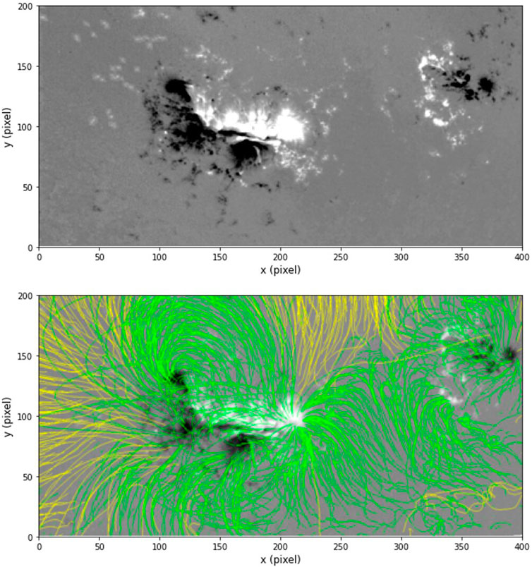
FIGURE 1. (Top) The HMI measured magnetogram from 2012-03-07 00:00UT. (Bottom) The NLFFF extrapolated from the 00:00UT magnetogram.

3.2 Flare brightening

The SDO Advanced Imaging Assembly (AIA) (Lemen et al., 2012) provides nearly simultaneous full-disk images of the corona and transition region—up to 0.5 solar radii above the solar limb—from 10 different wavelength channels with 1.5 arcsec spatial resolution and 12 s temporal resolution. The AIA 171 Å channel captures emissions from Fe ix ions at temperatures around 0.6 MK, showing the quiet corona and upper transition region. The AIA 211 Å channel captures emissions from Fe xiv ions at temperatures around 2 MK, showing the active region corona. The AIA 1600 Å channel captures emissions from C iv ions at temperatures around 10,000 K, showing the upper photosphere and lower transition region. Areas of flare brightening were determined by the overlap of the brightest areas seen in the SDO/AIA 171 Å, 211 Å, and 1,600 Å imagery. To find such areas, imagery from the three AIA channels—for the same field-of-view (FOV) as that of the magnetogram—were overlaid using the JHelioviewer tool (Müller et al., 2017; see Figure 2). The 1,600 Å imagery was set to the red channel; the 171 Å imagery was set to the green channel; and the 211 Å imagery was set to the blue channel for the overlaid image. Pixels (within the same boxed area shown in Figure 2) that had RGB values greater than or equal to 250—i.e., overlapping bright pixels from the three AIA images—identified the areas of flare brightening. Figure 3 illustrates the evolution of the cumulative area of flare brightening from the start of the X5.4 flare through 1 hour after. The cumulative area is very similar to the cumulative flare ribbon from Kazachenko et al. (2017). The alignment between areas of flare brightening and regions of strong surface magnetic field strength and high twist was compared to test the predictive capability of such regions in identifying flare location.

FIGURE 2

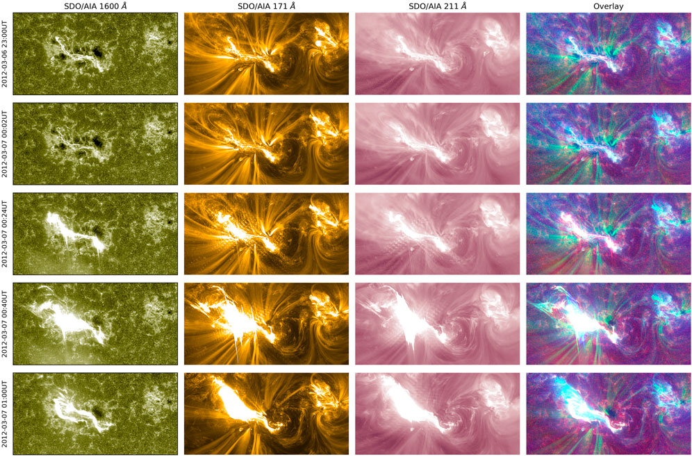
FIGURE 2. Imagery from the 1,600 Å, 171 Å, and 211 Å AIA channels, as well as the overlaid image, for (1st row) 1 hour before flare start, (2nd row) flare start time, (3rd row) 6 minutes after flare start, (4th row) flare max time, and (5th row) flare start time.

FIGURE 3

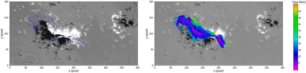
FIGURE 3. (Left) Contour of the cumulative area of flare brightening from flare start through 1 hour after flare overlaid on the 2012-03-07 00:00UT magnetogram. (Right) Evolution of flare brightening for the same time period.

3.3 Data volumes

The following regions were identified and used as masks to generate separate data volumes for magnetic field parameter calculations.

1) Active Region—AR

2) Overlap of strong surface magnetic field strength and high twist (Overlap Region)—OR

Concerning the data volumes, the AR was defined as the areas where the magnitude of the observed component of the photospheric magnetic field, normal to the surface, |B_z|, is greater than or equal to 300 G (G) within the boxed portion of the magnetogram (see Figure 4). The threshold is slightly higher than the typical threshold range of 100—200 G seen in other studies to avoid noisy, weak field data (Bobra et al., 2014; Kazachenko et al., 2017; Kazachenko et al., 2022).

FIGURE 4

FIGURE 4. (Top) The HMI measured magnetogram from 2012-03-07 00:00UT with box around NOAA AR 11429. (Bottom) The 00:00UT AR defined as region with |B_z|≥ 300 G within the boxed in area.

The OR was defined as areas within the same boxed portion as before, with the observed surface (or photospheric) |B| ≥ 1000 G and |T_w|≥ 1.5 turn, where T_w is the twist number of individual field lines calculated using the code developed by Liu et al. (2016). The magnetic field strength threshold is the same as that used in Kusano et al. (2020). The threshold for |T_w| is a common threshold used and considered appropriate to define moderate to high twist. The purpose of the OR was to isolate the portions of the magnetic field involved with the flaring process, as well as investigate if the observed photospheric measurements of field strength and twist can be used to identify the location of flaring within an AR. Figure 5 suggests that the OR aligns quite well with the initial areas of brightening seen in AIA imagery.

FIGURE 5

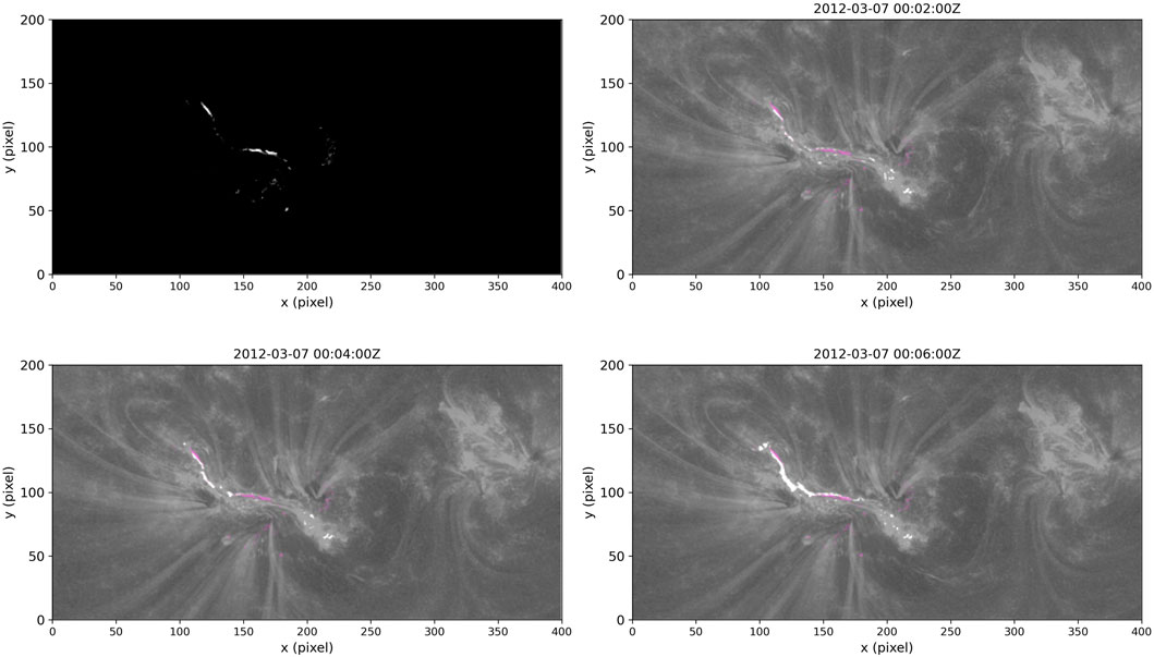
FIGURE 5. (Top Left) The 00:00UT OR defined as region with |B|≥ 1000 G and |T_w|≥ 1.5 turn within the same boxed in area as before. (Top Right and Bottom) The OR (purple shading) overlaid on the areas of initial flare brightening.

The 00:00UT AR and OR—i.e., the AR and OR at the time closest to when the flare was triggered—were used to determine magnetic field line seed locations—i.e., the locations of the photospheric footprints of the field lines. From these seed locations, the field lines within the [400,200,200] box were traced using linear interpolation, as part of the GX Simulator package (Nita et al., 2015; Nita et al., 2018). The coordinates of the field lines identify the volume elements used to calculate the magnetic field parameters—i.e., the data volumes. Data volumes were generated (using the specified seed locations) for each of the 11 extrapolated magnetic fields throughout the time period around the solar flare event. Figure 6, 7 shows the 00:00UT OR data volume.

FIGURE 6

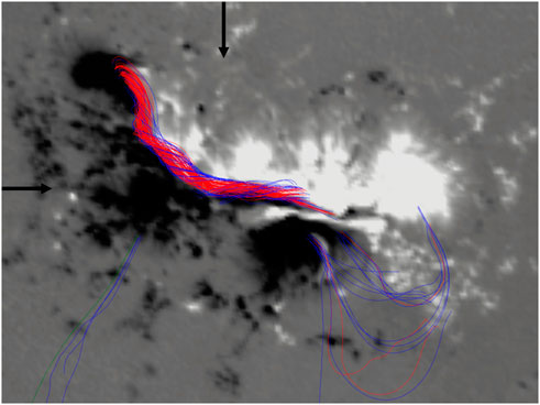
FIGURE 6. The 00:00UT OR data volume plotted over the 00:00UT magnetogram. Blue lines indicate closed field lines with 1.5 $\le |T_{\text{w}}|<$ 2.0, red lines indicate closed field lines with |T_w|≥ 2.0, and green lines indicate open field lines. Note that the open field lines are lines that extend out of the [400,200,200] box and do not necessarily open to interplanetary space. The arrows at the top and on the side represent the center lines of the xz-plane and yz-plane views, respectively, seen in Figure 7.

FIGURE 7

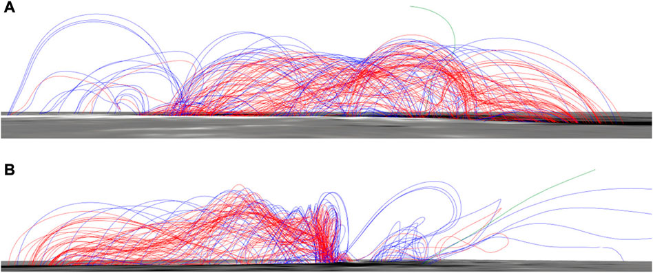
FIGURE 7. The xz-plane (A) and yz-plane (B) views of the 00:00UT OR data volume.

3.4 Magnetic field parameters

The magnetic field parameters calculated from the data volumes include four Space weather HMI Active Region Patch (SHARP) parameters—total unsigned flux (ϕ), total unsigned vertical current $(J_{{\text{z}}_{\text{Total}}})$, total unsigned current helicity $(H_{{\text{c}}_{\text{Total}}})$, and absolute value of the net current helicity (Hc_Abs)—as well as the total vertical magnetic field energy $(E_{{\text{B}}_{\text{Z}}})$, total vertical field gradient $(\nabla B_{{\text{z}}_{\text{Total}}})$, and total unsigned magnetic twist flux (τ_Total). The description, units, and formulas for the seven magnetic field parameters are listed in Table 2. The summations for the parameters occur over the individual volume elements within the different data volumes, with the exception of ϕ which is the surface flux. The SHARP parameters investigated were selected due to the potential predictive capability of these parameters found by Bobra and Couvidat (2015). The inclusion of the parameter τ is motivated by the predictive capability of the parameter found by Kusano et al. (2020).

TABLE 2

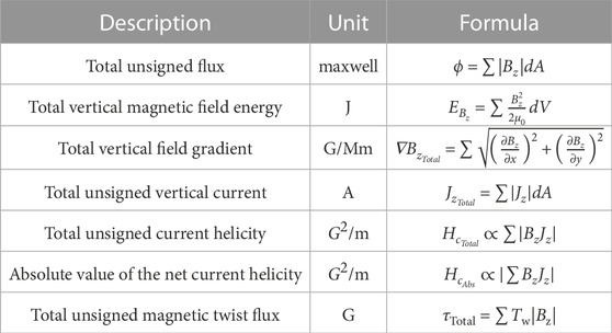
TABLE 2. The seven investigated magnetic field parameters with associated descriptions, units, and calculations.

To effectively compare the solar flare events and changes relative to flare occurrence, all parameters were normalized to the value at the flare start time. Time series of every parameter for each region (AR and OR) were plotted using the normalized values. Additionally, the error in each parameter was estimated using the same error analysis used for the total-based SHARP parameters (Bobra et al., 2014).

3.5 Twist structure

While α and τ provide a quantification of the overall twist calculated from the field values, it is important to examine the actual twist structure and how it evolves during the solar flare event. To accomplish this, twist maps—like that of Liu et al. (2016) and Yurchyshyn et al. (2022)—were calculated at vertical planes across and along the densest area of the OR and flare brightening, as well as in an area of weak magnetic field for reference (see Figure 8). For this flare event the area aligned well with the PIL, implying the eruption occurred directly over the PIL as opposed to the sliding eruption seen by Yurchyshyn et al. (2022). A highly twisted structure—likely a MFR—is evident in Figure 9 (shown by dark-blue areas of high twist) over the inversion line. The quantification and evolution of the twist structure was analyzed using the same sign-singularity measure (SSM) as that of Yurchyshyn et al. (2022). The SSM is calculated by:

$SSM\left(r\right)=\sum _{L_i\left(r\right)}|{\mu }_i\left(r\right)|,(4)$

where,

${\mu }_i\left(r\right)=\frac{{\int }_{L_i\left(r\right)}U\left(x,y\right)dxdy}{{\int }_{L_i\left(R\right)}U\left(x,y\right)dxdy}.(5)$

U (x, y) is the studied signed parameter (in this case T_w), and L_i(r) ⊂ L_i(R) represents a unique hierarchy of disjoint squares of size r, which cover the whole square L of size R that bounds the area of interest (Yurchyshyn et al., 2022).

FIGURE 8

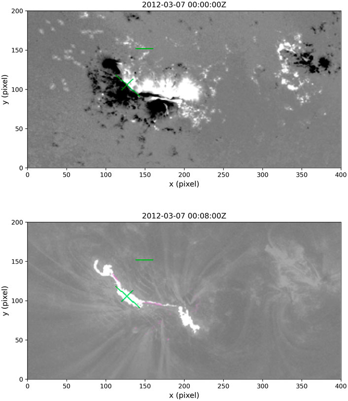
FIGURE 8. 2012-03-07 00:00UT magnetogram (Top) and 00:08UT AIA overlay image (grayscale) with OR represented by purple shading (Bottom). The green lines indicate the locations where the vertical twist maps were calculated, across and along the PIL, as well as in area of quieter magnetic activity (upper line).

FIGURE 9

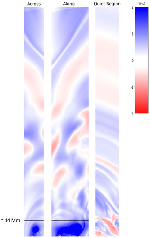
FIGURE 9. Vertical twist maps corresponding to the slices in Figure 8, calculated from the 2012-03-07 00:00UT extrapolated magnetic field. The black line on the twist maps calculated across and along the PIL indicates the top of the MFR structure at an altitude around 14 Mm.

4 Case study results

4.1 OR—Flare location

As mentioned in the previous section, the area within the AR with observed surface |B| ≥ 1000 G and |T_w|≥ 1.5 turn—i.e., the OR—aligns well with the area of initial brightening in SDO/AIA 171 Å, 211 Å, and 1,600 Å imagery during the onset of flaring (Figure 5). During the first couple minutes following flare initiation (from 00:02UT through 00:06UT), 45% of the bright pixels from the AIA imagery are encapsulated by or within 2 pixels of the OR; 67% are encapsulated or within 5 pixels; and 78% are encapsulated or within 10 pixels. As the X-ray flux quickly increases during the eruptive phase and pixels in the AIA imagery become saturated from the eruption, the area of brightening significantly outgrows the OR. However, the alignment throughout the pre-flare phase and beginning of the eruptive phase suggests that measurements of the photospheric magnetic field strength along with the twist calculated from the field measurements has the potential to provide a good indication of the flare location within an AR if triggered.

4.2 Twist structure evolution

Figure 10 shows the vertical twist maps at each timestep from 1 hour before through 1 hour after the X5.4 solar flare, as well as the X-ray flux measured by GOES during this time window. It is evident from the figure that a MFR - defined as areas with |T_w|≥ 1 - was present in the pre-eruptive magnetic field configuration, decayed slightly between the start and max of the flare, then decayed significantly following the peak and release of the associated CME. As the MFR decays following the eruption, twist higher in the corona is enhanced. Figure 11 shows the sign-singularity measure curves calculated from the vertical twist maps, as well as the time series of the total sign-singularity measure, which was calculated as the area under the different curves. The time series provides a quantification of the twist structure evolution visualized in Figure 10. The initial decrease in the total sign-singularity measure indicates the MFR becoming more coherent right up until the eruption, at which point an expected increase in the measure is seen as a result of the decaying MFR and overall fragmentation of the twist structure (Yurchyshyn et al., 2022).

FIGURE 10

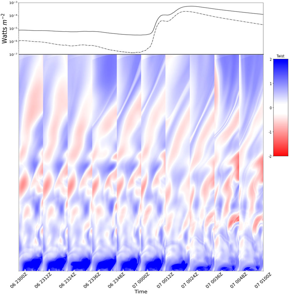
FIGURE 10. GOES measured X-ray flux combined with the vertical twist maps along the OR from 1 h before through 1 h after the X5.4 solar flare. The solid line represents the XRS long (1.0—8.0 Å) channel; the dashed line represents the short (0.5—4.0 Å) channel.

FIGURE 11

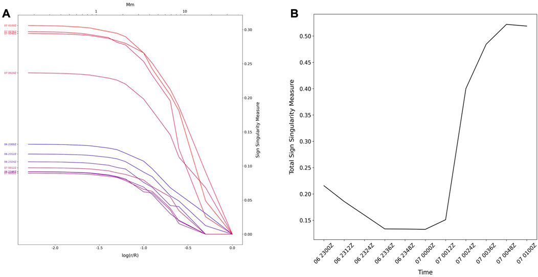
FIGURE 11. (A) Sign-singularity measure curves calculated from the vertical twist maps shown in Figure 10 and (B)the time series of the total sign-singularity measure (calculated as the area under the curves).

4.3 Magnetic field parameters time series

Figure 12 shows the temporal evolution of the seven investigated magnetic field parameters calculated from the extrapolated magnetic field. As mentioned in Section 3.4, for each parameter the values have been normalized to the value at the HARP data time nearest the start time of the solar flare—in this case 2012-03-07 00:00UT.

FIGURE 12

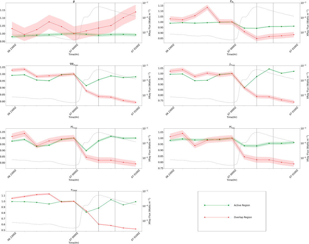
FIGURE 12. Time series of the seven magnetic field parameters calculated for each data volume, normalized to the values at the HARP data time closest to the start time of the X5.4 solar flare. The grey, dashed line is the GOES measured X-ray flux from the XRS long (1.0—8.0 Å) channel; the vertical, black dashed lines represent the GOES recorded start, max, and end time of the flare. The colored areas around the data points represent the error bounds.

The AR experiences a fairly consistent increase of about 2% in ϕ, with a peak flux just before the start of the flare. Conversely, the OR experiences a decrease of about 8% in ϕ, with a minimum just before the start of the flare and a fairly consistent increase throughout the duration of the event. The AR also experiences a peak in $E_{{\text{B}}_{\text{z}}}$ just before the start of the flare, followed by a rapid decrease of 6% just after the start. The OR experiences a maximum in $E_{{\text{B}}_{\text{z}}}$ 24 min before the flare start, then an overall decrease of approximately 28% through the maxtime of the flare. The peak in ϕ and $E_{{\text{B}}_{\text{z}}}$ for the OR 24 min prior to the start of the flare is likely the result of field lines in close proximity to the MFR—that initially were part of the strapping field—being stretched and sheared until magnetic reconnection occurred, causing them to wrap around the axis of the MFR. As all these field lines become part of the MFR, winding along the full length of it, the once more vertically oriented loop structures become elongated in the horizontal. The rest of the strapping field—with footprints further from the axis of the MFR—continue to be stretched in the vertical, hence the steady increase in the parameters for the AR up to a maximum just before the flare start. Once the instability of the magnetic field reaches the point to trigger the eruption, energy is lost and the field near the point of eruption begins to relax to a less stressed state. The AR field directly over the decaying MFR is no longer stretched as extensively, and the OR field re-configures to more simple loop structures.

The OR experiences a 20%–25% reduction in $\mathrm{\nabla }{B}_{{\text{z}}_{\text{Total}}}$, $J_{{\text{z}}_{\text{Total}}}$, $H_{{\text{c}}_{\text{Total}}}$, and $H_{{\text{c}}_{\text{Abs}}}$, and a 50% reduction in τ_Total after the eruption, with post-flare values remaining lower than pre-flare values. The AR experiences only a 8%–12% reduction in $\mathrm{\nabla }{B}_{{\text{z}}_{\text{Total}}}$, $J_{{\text{z}}_{\text{Total}}}$, $H_{{\text{c}}_{\text{Total}}}$, and $H_{{\text{c}}_{\text{Abs}}}$, and a 20% reduction in τ_Total. Furthermore, throughout the remaining duration of the flare event, the AR sees an increase in all the of the parameters to values around or just above the pre-flare values. The increase to pre-flare values seen for AR but not the OR suggests that while the portions of the magnetic field involved in the flaring process (OR) relax to a less stressed state following the onset of the solar flare, the eruptive motions can enhance the complexity of the magnetic field over other sections of the AR further from the point of eruption, consistent with the findings of Verma (2018) and Garland et al. (2022).

5 Conclusion

The X5.4 solar flare—with an associated CME—that occurred on 7 March 2012 from NOAA AR 11429 is a prime example of the standard or “two-ribbon” flare model. From the twist structure evolution and the flare ribbons present in the AIA 1600 Å imagery (Figure 3), it is clear that a MFR—which either emerged from the solar interior as such or resulted from the transition of a SMA (Patsourakos et al., 2020)—developed directly over the PIL of NOAA AR 11429, with its axis aligned with the PIL. As indicated by the evolution of the 7 parameters calculated for the separate portions of the magnetic field (AR and OR) throughout the 2-h window around the flare start, field lines near the MFR underwent reconnection, becoming part of the MFR and increasing the instability of the magnetic field structure. Following the eruption, many of the twisted field lines and coronal plasma tied to them were released with the flare/CME, and the field near the PIL began to unwind and relax to a less stressed state. The eruptive motions of the flare/CME enhanced the complexity of the magnetic field further from the point of eruption.

The results of this case study demonstrated that the outlined procedure has potential for accomplishing the goal of improving predictive capabilities of solar flares. The OR aligns well with areas of initial flare brightening, suggesting the observed photospheric magnetic field strength and twist together provide a good indication of where the eruption will take place within an AR, in line with the findings of Kusano et al. (2020). The evolution of the investigated magnetic field parameters for the separate regions (AR and OR) did indicate a destabilizing magnetic field structure that could likely erupt. However, given that this was only a case study, it cannot be concluded that any of the pre-flare trends provide a discriminating signature or clear predictor of flare occurrence. To determine if any of the trends seen for this case study hold true for all cases, or all cases of similar sunspot/magnetic classification, requires performing the same analysis on a large dataset, which will be conducted in the future.

Data availability statement

Publicly available datasets were analyzed in this study. This data can be found here: http://jsoc.stanford.edu/ajax/exportdata.html.

Author contributions

SG is the leader of the study and proposed the original idea; VY provided instruction with simulations; VY and DE provided assistance with code development; VY, RL, BA, and DE all provided general guidance.

Funding

This research was funded by the Air Force Office of Scientific Research (AFOSR/RTB1). The views, opinions, and/or findings expressed are those of the author and should not be interpreted as representing the official views or policies of the Department of Defense or the U.S. Government. VY acknowledges support from NSF AST-1614457, AGS-1954737, AST-2108235, AFOSR FA9550-19-1-0040, NASA 80NSSC17K0016, 80NSSC19K0257, and 80NSSC20K0025 grants.

Acknowledgments

We thank referees for careful reading the manuscript and providing valuable criticism and suggestions.

Conflict of interest

The authors declare that the research was conducted in the absence of any commercial or financial relationships that could be construed as a potential conflict of interest.

Publisher’s note

All claims expressed in this article are solely those of the authors and do not necessarily represent those of their affiliated organizations, or those of the publisher, the editors and the reviewers. Any product that may be evaluated in this article, or claim that may be made by its manufacturer, is not guaranteed or endorsed by the publisher.

References

Amari, T., Aly, J., Luciani, J., Boulmezaoud, T., and Mikic, Z. (1997). Reconstructing the solar coronal magnetic field as a force-free magnetic field. Sol. Phys. 174, 129–149. doi:10.1023/a:1004966830232

CrossRef Full Text | Google Scholar

Barnes, G., Leka, K. D., Schrijver, C. J., Colak, T., Qahwaji, R., Ashamari, O. W., et al. (2016). A comparison of flare forecasting methods. I. Results from the “all-clear” workshop. Astrophysical J. 829, 89. doi:10.3847/0004-637x/829/2/89

CrossRef Full Text | Google Scholar

Bobra, M. G., and Couvidat, S. (2015). Solar flare prediction using SDO/HMI vector magnetic field data with a machine-learning algorithm. Astrophysical J. 798, 135. doi:10.1088/0004-637x/798/2/135

CrossRef Full Text | Google Scholar

Bobra, M. G., Sun, X., Hoeksema, J. T., Turmon, M., Liu, Y., Hayashi, K., et al. (2014). The helioseismic and magnetic imager (HMI) vector magnetic field pipeline: SHARPs–space-weather HMI active region patches. Sol. Phys. 289, 3549–3578. doi:10.1007/s11207-014-0529-3

CrossRef Full Text | Google Scholar

Couvidat, S., Schou, J., Hoeksema, J. T., Bogart, R. S., Bush, R. I., Duvall, T. L., et al. (2016). Observables processing for the helioseismic and magnetic imager instrument on the solar dynamics observatory. Sol. Phys. 291, 1887–1938. doi:10.1007/s11207-016-0957-3

CrossRef Full Text | Google Scholar

Davies, K. (1990). “Electromagnetic waves (institution of engineering and technology),” in Ionospheric radio (London: IET Digital Library). doi:10.1049/PBEW031E

CrossRef Full Text | Google Scholar

Eastwood, J., Biffis, E., Hapgood, M., Green, L., Bisi, M., Bentley, R., et al. (2017). The economic impact of space weather: Where do we stand? Risk Anal. 37, 206–218. doi:10.1111/risa.12765

PubMed Abstract | CrossRef Full Text | Google Scholar

Fleishman, G. D., Anfinogentov, S., Loukitcheva, M., Mysh’yakov, I., and Stupishin, A. (2017). Casting the coronal magnetic field reconstruction tools in 3D using the MHD bifrost model. Astrophysical J. 839, 30. doi:10.3847/1538-4357/aa6840

CrossRef Full Text | Google Scholar

Garland, S. H., Emmons, D. J., and Loper, R. D. (2022). Studying the conditions for magnetic reconnection in solar flares with and without precursor flares. J. Atmos. Solar-Terrestrial Phys. 227, 105788. doi:10.1016/j.jastp.2021.105788

CrossRef Full Text | Google Scholar

Gupta, M., Thalmann, J. K., and Veronig, A. M. (2021). Magnetic helicity and energy budget around large confined and eruptive solar flares. Astronomy Astrophysics 653, A69. doi:10.1051/0004-6361/202140591

CrossRef Full Text | Google Scholar

Inoue, S., Kusano, K., Magara, T., Shiota, D., and Yamamoto, T. T. (2011). Twist and connectivity of magnetic field lines in the solar active region NOAA 10930. Astrophysical J. 738, 161. doi:10.1088/0004-637x/738/2/161

CrossRef Full Text | Google Scholar

Jing, J., Liu, C., Lee, J., Ji, H., Liu, N., Xu, Y., et al. (2018). Statistical analysis of torus and kink instabilities in solar eruptions. Astrophysical J. 864, 138. doi:10.3847/1538-4357/aad6e4

CrossRef Full Text | Google Scholar

Joint Science Operations Center (2020). Harp - HMI active region patches. Available at: http://jsoc.stanford.edu/jsocwiki/HARPDataSeries.

Google Scholar

Kazachenko, M. D., Lynch, B. J., Savcheva, A., Sun, X., and Welsch, B. T. (2022). Toward improved understanding of magnetic fields participating in solar flares: Statistical analysis of magnetic fields within flare ribbons. Astrophysical J. 926, 56. doi:10.3847/1538-4357/ac3af3

CrossRef Full Text | Google Scholar

Kazachenko, M. D., Lynch, B. J., Welsch, B. T., and Sun, X. (2017). A database of flare ribbon properties from the solar dynamics observatory. i. reconnection flux. Astrophysical J. 845, 49. doi:10.3847/1538-4357/aa7ed6

CrossRef Full Text | Google Scholar

Kusano, K., Iju, T., Bamba, Y., and Inoue, S. (2020). A physics-based method that can predict imminent large solar flares. Science 369, 587–591. doi:10.1126/science.aaz2511

PubMed Abstract | CrossRef Full Text | Google Scholar

Leka, K., and Barnes, G. (2007). Photospheric magnetic field properties of flaring versus flare-quiet active regions. iv. a statistically significant sample. Astrophysical J. 656, 1173–1186. doi:10.1086/510282

CrossRef Full Text | Google Scholar

Leka, K., Barnes, G., and Wagner, E. (2018). The NWRA classification infrastructure: Description and extension to the discriminant analysis flare forecasting system (DAFFS). J. Space Weather Space Clim. 8, A25. doi:10.1051/swsc/2018004

CrossRef Full Text | Google Scholar

Leka, K. D., and Barnes, G. (2003). Photospheric magnetic field properties of flaring versus flare-quiet active regions. II. discriminant analysis. Astrophysical J. 595, 1296–1306. doi:10.1086/377512

CrossRef Full Text | Google Scholar

Leka, K. D., Park, S.-H., Kusano, K., Andries, J., Barnes, G., Bingham, S., et al. (2019). A comparison of flare forecasting methods. III. systematic behaviors of operational solar flare forecasting systems. Astrophysical J. 881, 101. doi:10.3847/1538-4357/ab2e11

CrossRef Full Text | Google Scholar

Lemen, J. R., Title, A. M., Akin, D. J., Boerner, P. F., Chou, C., Drake, J. F., et al. (2012). The atmospheric imaging assembly (AIA) on the solar dynamics observatory (SDO). Sol. Phys. 275, 17–40. doi:10.1007/s11207-011-9776-8

CrossRef Full Text | Google Scholar

Liu, R., Kliem, B., Titov, V. S., Chen, J., Wang, Y., Wang, H., et al. (2016). Structure, stability, and evolution of magnetic flux ropes from the perspective of magnetic twist. Astrophysical J. 818, 148. doi:10.3847/0004-637x/818/2/148

CrossRef Full Text | Google Scholar

Mason, J. P., and Hoeksema, J. T. (2010). Testing automated solar flare forecasting with 13 Years of michelson Doppler imager magnetograms. Astrophysical J. 723, 634–640. doi:10.1088/0004-637x/723/1/634

CrossRef Full Text | Google Scholar

McIntosh, P. S. (1990). The classification of sunspot groups. Sol. Phys. 125, 251–267. doi:10.1007/bf00158405

CrossRef Full Text | Google Scholar

Müller, D., Nicula, B., Felix, S., Verstringe, F., Bourgoignie, B., Csillaghy, A., et al. (2017). JHelioviewer. Time-dependent 3D visualisation of solar and heliospheric data. Astronomy Astrophysics 606, A10. doi:10.1051/0004-6361/201730893

CrossRef Full Text | Google Scholar

Nita, G. M., Fleishman, G. D., Kuznetsov, A. A., Kontar, E. P., and Gary, D. E. (2015). Three-dimensional radio and X-ray modeling and data analysis software: Revealing flare complexity. Astrophysical J. 799, 236. doi:10.1088/0004-637x/799/2/236

CrossRef Full Text | Google Scholar

Nita, G. M., Viall, N. M., Klimchuk, J. A., Loukitcheva, M. A., Gary, D. E., Kuznetsov, A. A., et al. (2018). Dressing the coronal magnetic extrapolations of active regions with a parameterized thermal structure. Astrophysical J. 853, 66. doi:10.3847/1538-4357/aaa4bf

CrossRef Full Text | Google Scholar

Patsourakos, S., Vourlidas, A., Török, T., Kliem, B., Antiochos, S., Archontis, V., et al. (2020). Decoding the pre-eruptive magnetic field configurations of coronal mass ejections. Space Sci. Rev. 216, 131. doi:10.1007/s11214-020-00757-9

CrossRef Full Text | Google Scholar

Pu, Z., and Kalnay, E. (2018). “Numerical weather prediction basics: Models, numerical methods, and data assimilation,” in Handbook of hydrometeorological ensemble forecasting (Heidelberg: Springer Berlin Heidelberg). doi:10.1007/978-3-642-40457-3_11-1

CrossRef Full Text | Google Scholar

Valori, G., Kliem, B., and Keppens, R. (2005). Extrapolation of a nonlinear force-free field containing a highly twisted magnetic loop. Astronomy Astrophysics 433, 335–347. doi:10.1051/0004-6361:20042008

CrossRef Full Text | Google Scholar

Verma, M. (2018). The origin of two X-class flares in active region NOAA 12673-shear flows and head-on collision of new and preexisting flux. Astronomy Astrophysics 612, A101. doi:10.1051/0004-6361/201732214

CrossRef Full Text | Google Scholar

Wheatland, M. S., Sturrock, P. A., and Roumeliotis, G. (2000). An optimization approach to reconstructing force-free fields. Astrophysical J. 540, 1150–1155. doi:10.1086/309355

CrossRef Full Text | Google Scholar

Whitney Aegerter, T. R., Emmons, D. J., and Loper, R. D. (2020). Detection of reconnection signatures in solar flares. J. Atmos. Solar-Terrestrial Phys. 208, 105375. doi:10.1016/j.jastp.2020.105375

CrossRef Full Text | Google Scholar

Wiegelmann, T., Petrie, G. J. D., and Riley, P. (2017). Coronal magnetic field models. Space Sci. Rev. 210, 249–274. doi:10.1007/s11214-015-0178-3

CrossRef Full Text | Google Scholar

Yurchyshyn, V., Yang, X., Nita, G., Fleishman, G., Abramenko, V., Inoue, S., et al. (2022). Magnetic field re-configuration associated with a slow rise eruptive x1.2 flare in noaa active region 11944. Front. Astronomy Space Sci. 9, 816523. doi:10.3389/fspas.2022.816523

CrossRef Full Text | Google Scholar