Observations key to understanding solar cycles: a review

1 Introduction

A paradigm is “A set of assumptions, concepts, values, and practices that constitutes a way of viewing reality for the community that shares them, especially in an intellectual discipline.” This review discusses solar cycles from the perspective of a paradigm shift on solar cycles now taking place. The evidence is from observations. A few solar cycle theories are mentioned in this review but are not discussed in detail. The reader is referred to a complementary review on theories of solar cycles by Weber et al. (2023) and other review articles referenced therein. In this limited review, solar observations are first discussed as occurring in eras that span decades of solar research and are identified as paradigms.

I suggest that the previous paradigm was stimulated by new magnetic field observations during the early days of the Mt. Wilson Observatory using spectroheliographs that were new at that time. Paramount among the early discoveries of the unique magnetic properties of sunspot cycles are 1) the discovery of the bipolar nature of sunspots and magnetic fields of their active regions, 2) the finding of opposite orientations in the northern and southern hemispheres with west-to-east orientations in the northern hemisphere in odd numbered sunspot cycles and east-to-west orientations in the northern hemisphere in even numbered cycles, with few exceptions, 3) the reversal of their dominant orientations at the beginning of each new sunspot cycle, and 4) the discovery of the two polar magnetic fields and their reversal in polarity during each 11-year solar maximum.

These magnetic properties of solar cycles found at the Mt. Wilson Observatory added to the properties learned from the previous 400 years of sunspot observations prior to our knowledge of their magnetic fields. The average sunspot cycle duration was 11 years. The number of sunspot groups increased to solar maximum over 3–4 years after the first sunspots appeared. The number declined over 5–6 years until few or no sunspots occurred during solar minimum. They occurred in two bands initially approximately 10–15° in width and increased to approximately 30° in latitude before decreasing again after solar maximum in both hemispheres. The initial sunspots were small, short-lived, and began approximately 30–40° in latitude. As the population of sunspots increased, a broadening of their distributions in size and latitude increased until solar maximum. After the maximum, the range in latitude decreased along with the decreasing population of sunspots until none remained near the equator at the end of the approximate 11 years of the cycle.

A puzzling difference between successive sunspot cycles was the complete change in the orientation of the magnetic fields of the sunspots and their surrounding bipolar magnetic fields by 180° with each new sunspot cycle (Hale et al., 2019; Hale and Nicholson, 1925). This meant the basic sunspot cycle length was approximately 11 years, but the complete magnetic cycle was two 11-year sunspot cycles.

The first articles to explicitly say that a new paradigm for solar cycles had emerged are by Srivastava et al. (2018) and McIntosh et al. (2021). The individual 20 researchers contributing to these articles recognize that the new paradigm was initiated in the article of McIntosh et al. (2014). Using proxies of EUV bright points for the large population of small active regions without sunspots, McIntosh et al. (2014) presented diagrams called “band-o-grams” showing two 22-year overlapping solar cycles present on the Sun continuously. In brief, this is a radically different perception from the 11-year average solar cycles described above. This paradigm shift is the finding of the true meaning of the 22-year magnetic cycle and re-identifying sunspots as phases in the 22-year cycles rather than independent cycles.

This change in perception of solar cycles from a single linear series of 11-year cycles to the realization that two complete overlapping 22-year cycles are always present on the Sun, is the substance of this review. Readers already familiar with solar cycles might choose to first read Section 4 on the extended solar cycle or Section 5 on the existence and ramifications of two 22-year, overlapping solar cycles. Sections 6–9 describes changed views on other aspects of solar cycles that could become a part of the new paradigm.

Section 2 briefly reviews and illustrates details learned about solar cycles from observing only sunspots.

Section 3 describes what was learned about sunspots and solar cycles when magnetic field measurements first became possible using the Mt. Wilson spectrographs and later the Babcock magnetograph.

Section 4 summarizes key details in the emergence of the concept of an extended solar cycle from magnetographs and instruments at various solar observatories.

Section 5 examines the existence and ramifications of two 22-year solar cycles continuously on the Sun.

Section 6 emphasizes the fundamental role of ephemeral active regions in understanding the 22-year Hale Solar Cycle. Section 6 also cites articles that conclude: the smallest bipolar structures of ephemeral region and larger active regions are the same features. They are named “elementary bipoles” because they appear to be the building blocks of all active regions.

Section 7 discusses observations relevant to identifying the source of the magnetic fields that migrate toward the poles and replace the polar fields around the maximum of the 11-year sunspot cycle.

Section 8 analyzes the evolution of magnetic fields with the potential for reversing the polarity orientation of the active regions at the beginning of every 22-year solar cycle.

Section 9 is the Discussion section; it presents a brief overview envisioning future solar cycle studies.

2 The solar cycle, as known from sunspots

Sunspots were observed by ancient cultures, and no individual can be given credit for their discovery. The historical record of sunspot cycles includes drawings made from naked-eye observations. An example is shown in Figure 1 made in the year 1618 and rediscovered by Wang and Li (2022). From this rediscovery, the authors could conclude a solar minimum, thought to have occurred in 1618, instead occurred in 1620. Such seemingly small details can be important; the cause of the 22-year solar cycle and longer periods in the variation of solar cycles remains one of the biggest unsolved puzzles in solar physics (Hathaway, 2015, a review).

FIGURE 1

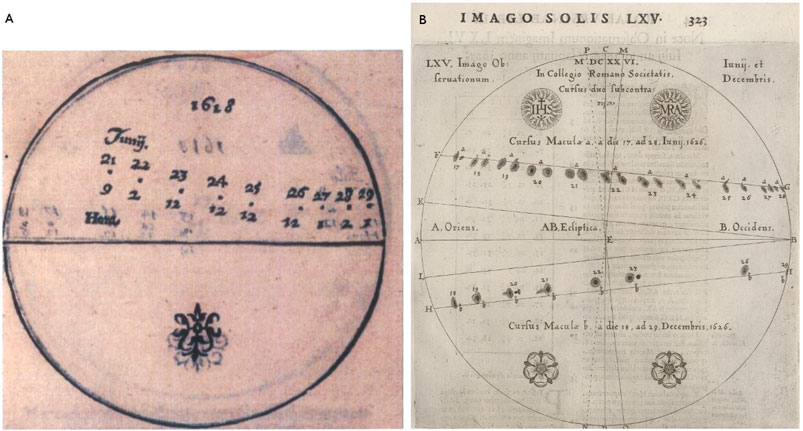
FIGURE 1. (A) Malapert drawing from the article “Rediscovery of 23 Naked-eye Sunspot Records.” As originally written on the drawing, the dates are 21 to 29 July 1618 as published by Wang and Li (2022). The drawing of a dot represents the daily progress of a sunspot as it crosses the solar disk at a rate of approximately 13° per day. Sunspots remain at relatively fixed locations on the Sun. The curved path of the sunspots reveals that the north solar pole is tilted toward Earth. The horizontal line is not the equator. One can assume this sunspot stays at the same latitude and distance from the equator within a degree or less. Therefore, in this drawing, the rotational axis of the Sun is tilted clockwise approximately 20°. (B) On the right is seen a similar, later series of drawings by Christoph Scheiner in Germany; a pair of sunspots in the northern hemisphere was traced in 1626 from June 1 through June 28. The straight line K at the left side of the solar disk shows where a line of constant latitude intersects the east limb of the Sun. In the southern hemisphere, another sunspot was drawn in similar detail from 18 to 29 December 1626. The tilt of the rotational axis of the Sun in the sky is in the opposite direction from the drawing in the northern hemisphere. Credit for (A): Wang and Li (2022). Credit for (B): the library at the University of Oslo which owns an original of the Book by Scheiner, “Rosa Ursina sive Sol.” The copied image was provided by the courtesy of Prof. Oddbjorn Engvold.

Sunspots large enough to be seen by the naked eye are approximately one-hundredth of the solar diameter. Sunspots, this large and larger, often appear as pairs of slightly distorted, dark disks with surrounding smaller sunspots. Their frequency of occurrence from solar maximum to solar minimum over the 11-year solar cycle is illustrated in Figure 2. These images from the Solar Dynamics Observatory were recorded during the solar maximum of solar cycle 23 on 19 July 2000 (Figure 2A) and during the next solar minimum on 18 March 2009 (Figure 2B).

FIGURE 2

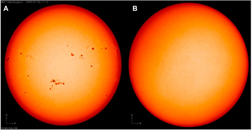
FIGURE 2. The image of (A) was recorded on 19 July 2000 during the maximum of solar cycle 23 and the image of (B) on 18 March 2009 during the following solar minimum. Credit: The Solar Dynamics Observatory and NASA.

Figure 1B on the right shows a similar later series of drawings by Christoph Scheiner in Germany; a pair of sunspots in the northern hemisphere was traced in 1626 from June 1 through June 28. The straight line, K at the left side of the solar disk, shows where a line of constant latitude intersects the east limb of the Sun. In the southern hemisphere, another sunspot was drawn in similar detail from 18 to 29 December 1626. The tilt of the rotational axis of the Sun in the sky is in the opposite direction from the drawing in the northern hemisphere (credit for Figure 1A: Wang and Li, 2022 and credit for Figure 1B: to the library at the University of Oslo, which owns an original of the Book by Scheiner, “Rosa Ursina sive Sol.” The copied image was provided by courtesy of Prof. Oddbjorn Engvold).

The discovery of the 11-year sunspot cycle in Western recorded history is usually credited to Schwabe (1844). However, the older sunspot drawings in China showed that sunspots were sufficiently long in duration that it is possible and also likely that earlier observers in cultures living close to nature would have discovered the sunspot cycle.

The sunspot cycle is commonly represented as a graph of sunspot number versus time as illustrated in Figure 3. To date, the observed sunspot numbers have exceeded the predictions for the first years of solar cycle 25. This difference between the observed and predicted sunspot numbers is sufficient reason for continuing research on solar cycles of our closest star.

FIGURE 3

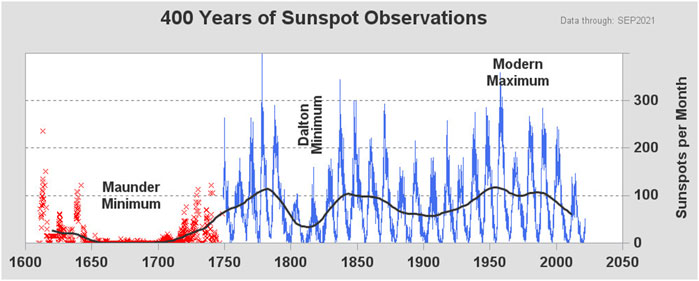
FIGURE 3. Sunspot number versus time that shows the variations from cycle to cycle over more than 400 years. The deep part of the Maunder Minimum lasted 70 years. The early part of current solar cycle 25 is shown at the right end of the graph. Credit: Space Weather Prediction Center.

Except for small motions in their growth phase, sunspots are relatively fixed in location. They frequently develop in pairs or small groups, as seen in Figure 1B by Scheiner, a co-temporary of Galileo (Engvold and Zirker, 2016). Their lifetimes are from a fraction of a day for small ones to several weeks for large ones, as shown in Figure 2. The longer apparent lifetimes are often observed in closely spaced groups of sunspots, repeatedly occurring at nearly the same latitudes and longitudes.

Changes in sunspots are readily seen daily as the Sun rotates around its central axis on average once every 27 days or approximately 13.5° per day. One can track some large sunspots across the 180° of the visible Sun realistically for up to 13 days. Figure 1 represents an example of three long-lived sunspots or sunspot groups. The tracking of sunspots like this one, four hundred or more years ago led astronomers to discover that the Sun’s speed of rotation is fastest at its equator and slowest at its highest latitudes, a phenomenon known as differential rotation. They found that one rotation of the Sun at its equator requires 25 days but increases to 29 days at 60° north and south latitudes.

The “butterfly” diagram in Figure 4 illustrates the gradual drift of the formation sites of sunspots from high to low latitudes over 13 complete sunspot cycles and two partial cycles. Although the average duration of a sunspot cycle is approximately 11 years, they can be as short as 9 years or as long as 14 years. Sunspots of a single cycle are first seen in both solar hemispheres at relatively high latitudes, up to approximately 40°. Throughout each solar cycle, successive sunspots gradually appear at lower and lower latitudes until they are close to the solar equator. A few appear to cross the equator as the ∼11-year sunspot cycle comes to an end. In Figure 4, one can see the band of latitudes, occupied by sunspots, widens until solar maximum and then narrow as the cycle declines. Sunspot cycles with the largest number also have the broadest distribution of sunspots in latitude. Some consecutive sunspot cycles overlap by 1–2 years but others do not overlap.

FIGURE 4

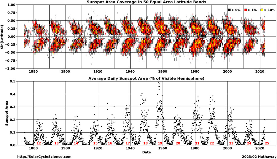
FIGURE 4. This “butterfly” diagram of 28 continuous 11-year sunspot cycles and two partial cycles reveals the range of latitudes of sunspots with time for both the northern and southern hemispheres. Sunspot cycles with the largest number of sunspots also have the broadest distribution of sunspots in latitude. Credit: David Hathaway, NASA Marshall Space Flight Center, Alabama, United States.

The above information about sunspot cycles was known before the year 1900. This was before Hale embarked successively on the construction of three of the largest solar spectroheliographs in the world at Mt. Wilson, California, United States, early in the 20th century. When sunspots were observed with the spectroheliographs, Hale and his colleagues found Zeeman splitting in solar spectral lines. This splitting was known to only occur in the presence of a magnetic field. From observing the Zeeman splitting, Hale and his colleagues could directly measure the strength and polarity of the magnetic fields of sunspots. The degree of Zeeman splitting is directly proportional to the magnetic field strength at the source on the spectrograph slit. The opposite polarizations, of the two split components of magnetically sensitive spectral lines, enabled the detection of sunspot polarity as either positive or negative. These measurements provided definitive evidence that sunspots are intense magnetic cores within the surrounding, larger magnetic fields in which they form. Hale and his colleagues measured magnetic fields ranging from 100 Gauss up to 2,300 Gauss (Hale and Nicholson, 1938). For more detailed information on sunspots, also see two books on sunspots by Bray and Loughhead (1964) and Loughhead and Bray (1979).

From all published information about sunspots, Babcock (1961) summarized five discoveries relevant to solar cycles. He presented them in the following order with credit to those who first discovered them. These discoveries are abbreviated here:

1. Differential rotation of the solar atmosphere, 25 days at the equator and 29.3 days at 60° north and south latitudes (Carrington, 1858).

2. An average 11-year rise and decline in the numbers of sunspots (Schwabe, 1844).

3. Limitation of sunspots to one band of latitudes in each hemisphere parallel to the solar equator (Carrington, 1858) and the slow progression of the bands toward the equator throughout the solar cycle (Sporer, 1894).

4. The bipolar character of sunspots. An imaginary line, from the centroid of sunspots of one polarity to the centroid of the opposite polarity, is aligned nearly parallel with the solar equator (Hale, 1913); the relative east–west orientations of the positive and negative polarities are opposite in the northern and southern hemispheres (Hale and Ellerman, 1918).

5. The reversal of the east–west polarity pattern of sunspots in both solar hemispheres at the beginning of every sunspot cycle. This led to the recognition of the Sun’s 22-year magnetic cycle consisting of two 11-year sunspot cycles (Hale et al., 1919; Hale and Nicholson, 1925).

From the images of the Sun recorded in various spectral lines, called spectroheliograms, early scientists studying the Sun could readily see sunspots were embedded in areas with bright and dark intricate structure. These larger areas bear the name “active regions.” This name is a catch-all for many types of dynamic solar events that occur in active regions, such as solar flares, surges, erupting prominences, and coronal mass ejections. Nearly all cyclical properties of sunspots are related to dynamic features produced in active regions.

In the early 1900s, daily observations of the Sun and its active regions and the associated features were also initiated at observatories around the world. Important, long-term, historic observations were taken at the Potsdam Observatory in Germany, the Kodaikanal Observatory in India, the Meudon Solar Observatory and Pic du Midi Observatory in France, and the Climax Observatory and Sacramento Peak Observatory in the United States. These major observatories have also recorded solar prominences above the solar limb and their counterpart as filaments on the solar disk. The reader is referred to other reviews and books for more historic details on solar cycle records (review on Solar Cycles by Hathaway, 2015; Solar Prominences by Tandberg-Hanssen, 1974, 1995; Sunspots by Loughhead and Bray, 1979; and Solar Prominences with editors Vial and Engvold, 2015).

With the construction of spectroheliographs, filtergraphs, specialized narrow-band filters, and other instruments around the world, the search for the cause of sunspots became a broader search for the cause of the magnetic fields of active regions. The search for the cause of the magnetic fields of active regions remains a goal fundamental to understanding solar cycles.

3 The solar cycle, as known from early magnetograms

Continuing the picture of the previous paradigm are two important findings about the solar cycle that emerged from data taken with the new Mt. Wilson magnetograph designed and built by H. D. and H. W. Babcock. Following the numbering of key observations in Section 2, these findings are

6. The existence of a main dipolar field (Babcock and Babcock, 1952).

7. The reversal of the polarity of the solar polar fields at the maximum of each solar cycle (Babcock and Livingston, 1958; Babcock, 1959).

The polar field was detected with certainty in 1951 (Babcock and Babcock, 1952) using the first Mt. Wilson magnetograph. Earlier attempts to detect the global magnetic field of the Sun had been made with other instruments but definitive observations were still required. The polar fields were found to be irregular in shape. Their overall area changed slowly over months, but their fine structure varied from day-to-day (Babcock and Babcock, 1952).

Large areas of magnetic fields of opposite polarity at the north and south poles slowly disappeared and were replaced by large areas of the opposite polarity magnetic field that had been migrating poleward. A surprising but slow reversal of the polarity of the polar magnetic fields took many months. The first observed reversal of the north and south polar fields was not simultaneous. The reversal of the north polar fields took place 1.1 years before the reversal occurred in the southern polar region (Babcock and Livingston, 1958; Babcock, 1959).

H. W. Babcock was well versed on the early knowledge of stellar magnetic fields as well as solar magnetic fields. Polarity reversals of the magnetic fields on stars had been found previously by Babcock (1947). His accumulation of knowledge became sufficient for him to confidently propose the first descriptive and semi-quantitative model of solar cycles (Babcock, 1961).

Babcock (1961) emphasized that only 1/2 of the 22-year solar cycle had been observed at that time. He said, “This attempt at a synthesis may be premature.” Babcock knew that changes had to be taking place on scales smaller than what the magnetograph could detect. That idea led him to work on instrument changes that would allow him to view the Sun in higher resolution. He also knew tiny sunspots in small bipolar regions outnumbered those in large active regions. He observed that solar cycles began with small bipolar regions and that their numbers increased with time as did the occurrence of larger regions. Looking ahead, he stated, “Of particular value would be more and better measurements of the distribution and quantity of magnetic flux in BMR (bipolar magnetic regions) as a function of age.”

In his original effort to explain the solar cycle, Babcock (1961) opens with, “shallow submerged lines of force of an initial axisymmetric dipolar field. . .” In his article, Babcock concluded that the active region magnetic fields could not be very deep for three reasons: a) the presence of more smaller, short-lived active regions than large long-lived ones, b) the migratory patterns of sunspot fields, and c) the replacement of fields of one polarity by opposite polarity fields. Babcock concluded that active region magnetic fields were not tied very deeply below the photosphere. He believed that they could float on the solar surface until opposite polarities merged or were “neutralized” and disappeared.

Since the time of Hale’s observations of solar magnetic fields, research on solar cycles has spread as new solar telescopes and spectroheliographs were developed at solar observatories around the world. Scientists at Mt. Wilson continued to be the leaders. Below are additional research findings, largely by Mt. Wilson scientists, taking observations with the Mt. Wilson spectrographs and magnetograph. In addition to the numbered points above, Babcock (1961) listed more findings that he thought required explanation in any future model of the 11-year solar cycle. This list is in the same order as in Babcock’s article. This list remains significant today. With more than 60 years of studies reviewed elsewhere (Petrovay, 2010, living review, on predicting solar cycles; Pesnell, 2012, solar cycle predictions, review; Cliver, 2014, extended solar cycle; Hathaway, 2015, review on solar cycles; and Martin, 2018, review on observational evidence of the depth at origin of active regions), these topics remain without definitive answers and important for further research:

8. The larger size and longer lifetime in the preceding (western) polarity sunspots than in the trailing (eastern) polarity sunspots in any solar cycle.

9. A forward tilt of the radial field of sunspots varying from 0.44° to 7.6° for sunspots of the oldest age.

10. The orientation of sunspot groups such that, on average, the leading (western) polarity in each hemisphere is closer to the equator than the trailing polarity.

11. The common recurrence of new sunspot groups at longitudes close to those of previous sunspots.

12. The bipolar magnetic regions underlying the development of sunspot groups and centers of activity (active regions).

13. The existence of hydrogen whirls which are groups of superpenumbral fibrils with a partial or complete spiral pattern around the periphery of many sunspots.

14. An ordered appearance for calcium flocculi, hydrogen flocculi, faculae, and sunspots. This sequence is the early evidence for concluding that active regions emerge from below the photosphere. It is largely supplanted now by more fundamental magnetic field data.

Item 13 warrants further explanation. Because sunspots were the first evidence of the existence of solar cycles, one would think that any feature closely related to sunspots might be a key to understanding solar cycles. Hale (1908) and Hale et al. (1919) were fascinated with H-alpha (hydrogen) images because the patterns of fine structure in active regions and around sunspots so closely resembled the lines of force around magnets on Earth. Daily observations were deemed essential for studying both short- and long-term changes in these solar structures. The images were recorded on glass plates using the Mt. Wilson spectroheliograph.

Richardson’s (1941) long-term study of the hydrogen whirls from the daily observations turned up surprising results that seemed to belie the expected solar cycle properties specifically associated with hydrogen whirls. As first discussed by Hale (1908), the degrees of curvature in the clockwise and counterclockwise directions of the hydrogen whirls were not proportional to the magnetic fields of the associated sunspots nor was the curvature associated with sunspot polarity.

Both clockwise and counterclockwise patterns were sometimes observed on a different part of the same sunspot of single polarity. An example is shown in the middle panel of Figure 5 from Balasubramaniam et al. (2004). There is a low degree of opposite curvature on both the east (left) side and west (right) side of the sunspot. The pattern on the right side of the sunspot in Figure 5B corresponds to the curvature of the schematic whirl in the left panel in Figure 5A from Martin (1998). Conversely, the pattern on the left side of the sunspot in Figure 5B corresponds to the schematic whirl in the panel on the right side of Figure 5A. This correspondence, of the curvature of the whirls around the sunspot to the schematic drawing of the chirality of filaments, is better seen if one mentally rotates the schematic drawing by 180° relative to the sunspot.

FIGURE 5

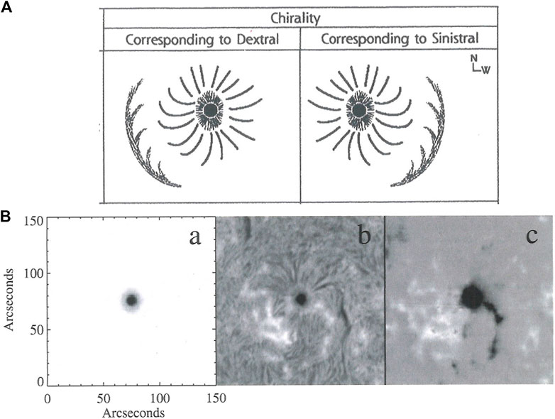
FIGURE 5. (A) Schematic drawing of hydrogen whirls revealed by sets of fibrils around sunspots. Dextral filaments are associated only with counterclockwise whirls as measured from the outer end of a fibril to the inner end of a sunspot. Sinistral filaments are associated only with clockwise whirls. The sign of whirls is independent of solar cycles (Richardson, 1941). Outside of the whirls around the sunspots, a dextral filament is schematically represented on the left and a sinistral filament on the right. Dextral and sinistral filaments and counterclockwise and clockwise whirls are related patterns of handedness known as chirality. Chiral patterns are mirror images of each other as illustrated here. (B) The dark feature to the right of the sunspot in the middle panel is a filament. Filaments closely follow the boundaries between areas of positive and negative polarity magnetic fields. White areas in the magnetogram on the right are positive polarity and black areas are negative polarity. Credits: (A) Martin, (1998, Figure 1). (B) Balasubramaniam et al. (2004, Figure 1).

Another new finding was a strong tendency for counterclockwise to be dominant in the northern hemisphere and clockwise in the southern hemisphere (Richardson, 1941). This finding of a hemispheric preference for hydrogen whirls is directly correlated with filaments as shown in Figure 5 and verified by Rust and Martin (1994), and Balasubramaniam et al. (2004). The chirality of the whirls around sunspots is determined by the horizontal component of the magnetic fields of filaments not the strong vertical magnetic field of sunspots. This is why Richardson found no relationship between the whirls and the magnitude of the magnetic fields in sunspots. Because of this lack of relationship of the hydrogen whirls and the magnitude of sunspots, one might think that there is no relationship between chirality and the solar cycle. However, there is a correlation between the hemispheric preference of chirality and the hemispheric preference of the hydrogen whirls. Dextral filaments and filament channels are most common in the northern hemisphere as are counterclockwise hydrogen whirls.

The definition of counterclockwise and clockwise given here for sunspots is from the outer end of each superpenumbral fibril furthest from the sunspot to the end closest to the sunspot (Richardson, 1941; Rust and Martin, 1994). This definition is consistent with the direction of the mass flows in the superpenumbral fibrils, which are toward the associated sunspot. The superpenumbral fibrils within a whirl of fibrils appear to originate in the chromosphere 10,000–30,000 km beyond the outer boundaries of sunspots.

In some articles, the whirls around a sunspot are called “superpenumbral fibrils.” The definition of the counterclockwise and clockwise direction along a fibril in a whirl in Balasubramaniam et al. (2004) is opposite to that by Richardson (1941). It is suggested that the Richardson’s definition become the standard definition as applied herein. The majority of authors, to date, have chosen to use the Richardson definition.

Hydrogen whirls are one of the several patterns of chirality (handedness) in solar features that do not reverse their hemispheric pattern every 11 years (Martin, 1998). At the present time, there is only one chiral pattern among solar features that appears to be related to the origin of solar cycles. That is the chirality of filaments and filament channels discussed in Section 8.

What should be clarified here is that the property of chirality has a physical significance that is rare. Features that possess the magnetic property of chirality have strict one-to-one relationships to each other but not necessarily to other solar conditions or properties. Claims of the lack of a one-to-one relationship have been proven to be incorrect due to a lack of sufficiently high spatial resolution (Martin, 2015). Chiral relationships have no exceptions. However, high-resolution observations are required for filament threads to be clearly seen. For example, counterclockwise whirls are always related to dextral filaments as illustrated by Rust and Martin (1994). This is always true and independent of other relationships, such as to solar hemisphere. By contrast, chiral relationships to hemisphere are statistical. There are exceptions. For example, counterclockwise hydrogen whirls were found by Richardson (1941) to be most common in the northern hemisphere while clockwise hydrogen whirls were most common in the southern hemisphere.

Exceptions have consistently been found to this hemispheric trend, first by Richardson (1941), and then by Martin (1998) and Balasubramaniam et al. (2004). We can identify relationships with exceptions as statistical relationships as distinct from one-to-one relationships which are invariable and linked to physical laws. This distinction is important because reliable predictions can be based on one-to-one relationships, whereas statistical relationships are inherently unreliable to some degree.

The reversal of the relative orientations of the positive and negative polarities of active regions with every new solar cycle is a statistical relationship. The polarities of individual active regions are sometimes reversed from the statistical tendency for most active regions to be either oriented east-to-west or west-to-east. There is a statistical tendency for up to 10% of individual active regions to be exceptions (Munoz-Jaramillo et al., 2022).

Babcock (1961) also tried to account for sufficient magnetic flux for large active regions. He followed Parker’s (1955) idea of the possible existence of submerged, but buoyant, toroidal, magnetic flux ropes below the photosphere. Babcock proposed the wrapping of such flux ropes by differential rotation in a shallow layer beneath the photosphere. To him, this was the best possible mechanism to bring rising loops of the submerged flux ropes to the photosphere where they would present as the bipolar magnetic fields of active regions. An important element in Babcock’s (1961) theory was finding the means of amplifying relatively weak magnetic fields of tens to hundreds of Gauss into fields of up to several thousand Gauss. Parker (1955) offered an amplification process that should occur in sunspots and Babcock made use of it in his grand scheme. This amplification is convective collapse, further investigated by Zwaan (1978) and others.

Multiple wrapping of subsurface magnetic fields around the Sun below the photosphere was originally proposed by Babcock (1961). His theoretical idea was to build subsurface flux ropes. The buoyancy of the flux ropes would allow small loops to rise and break through the photosphere to become active regions. It is now becoming evident that the processes of convection and reconnection, respectively, in the photosphere and outer layers of the solar atmosphere, are continuously reorganizing to achieve the simplest version of their dynamic state. The finding of supergranule-sized convection cells (Simon and Leighton, 1964; Leighton et al., 1962) in the outer one-third of the solar radius, along with increased knowledge of magnetic reconnection in different layers of the solar atmosphere, raises questions about the compatibility of these processes with the proposed long-term existence of the subsurface flux ropes (Martin, 2018).

Another process that locally amplifies magnetic flux has recently been identified by Chian et al. (2023). In observations from Hinode continuum intensity images and longitudinal magnetograms, it was seen that the magnetic field is intensified at the centers of two merging magnetic flux tubes trapped inside a vortex. The intensification had occurred during a 30-min interval during the vortex lifetime.

4 The extended solar cycle

At least three categories of observational studies are included in the concept of the extended solar cycle:

(a) Direct observations of small bipolar magnetic fields known as “ephemeral active regions” and

(b) EUV bright point data used as proxies for ephemeral active regions.

The second and third categories are only briefly mentioned in this review because an excellent review by Cliver (2014) on the extended solar cycle thoroughly discusses these important observations. These categories were first described by Wilson et al. (1988), who first used the term “extended solar cycle.”

The extended solar cycle also harks back to, and further extends, Babcock’s original lists of observations and results relevant to understanding solar cycles. Continuing with the numbering of these lists in Sections 2 and 3, I add more recent observations as an update to those cited by Babcock. The next item (15 below) is a fulfillment of Babcock’s stated desire for “more and better measurements of the distribution and quantity of BMR (bipolar magnetic regions) as a function of age:”

In the first category (direct observations of new magnetic flux):

15. Magnetic field observations of small active regions, usually without sunspots, and called “ephemeral active regions” (Harvey and Martin, 1973; Harvey et al., 1975; Martin and Harvey, 1979).

16. EUV bright points used as proxies for ephemeral regions at high latitudes (McIntosh et al., 2014; McIntosh and Leamon, 2017).

In the secondary category (related long-term changes in magnetic flux previously emerged):

17. Long-term records of filaments from Meudon and Pic du Midi Solar Observatories (Mazumder et al., 2021), Kodaikanal Observatory, (Chaterjee et al., 2020; Priyadarchi et al., 2022), and the McIntosh database (Mazumder, 2019; Mazumder et al., 2021).

18. Vector magnetic field information on solar filaments (Leroy et al., 1984; Bommier et al., 1994).

19. Coronal features observed in the green coronal line (Altrock, 1988; Altrock, 1997; Robbrecht et al., 2010).

20. Variations (also known as torsional oscillations) in zonal flows, found in exacting measurements of differential rotation (Snodgrass, 1987).

In hindsight, a door to the new paradigm on solar cycles was first opened when a magnetograph was constructed in the early 1970s at Kitt Peak. It was designed to produce daily magnetograms of the full solar disk at a spatial resolution that exceeded other full-disk magnetographs of that time. Harvey and Martin (1973) initiated systematic studies of the surprisingly large numbers of very small bipolar regions that were revealed in the new magnetograms.

For their studies of ephemeral active regions, Harvey and Martin (1973) chose all new bipolar regions which were a) not present on the previous day, b) did not develop obvious sunspots, and c) could still be observed on the following day. The last criterion allows the observer to be certain that happenstance encounters of opposite polarity fields are not being included. They adopted the name “ephemeral active regions” first used by Dodson in the early 1950s (Harvey, 2000) for the small bipolar active regions. A few such “ephemeral” regions had been designated among lists of larger active regions published in Solar Geophysical Data by the National Oceanic and Atmospheric Administration in the United States. Most ephemeral active regions survive 1 or 2 days. The designation “ephemeral”, however, implied that these active regions were of no importance because they were too small and short-lived to develop significant sunspots or solar flares.

Harvey and Martin (1973), Harvey et al. (1975), and Martin and Harvey (1979), however, found that ephemeral regions provided information about the solar cycle not yet known from either sunspots or larger and long-lived active regions. Harvey and Martin (1973) found that the ephemeral regions a) were more broadly distributed in latitude than larger active regions, b) displayed a much broader range of orientations of the axes of their bipolar magnetic fields than larger active regions, and c) had a majority that possessed the west-to-east or east-to-west orientation of the solar cycle to which they belonged.

The latitude distribution of ephemeral active regions is so broad that the question has been often raised: do all ephemeral active regions belong to solar cycles, or is there a component of small bipolar regions that are independent of solar cycles? Harvey et al. (1975) answered this question by systematically studying every observable property of ephemeral regions without sunspots to see if they shared the same characteristics as the larger active regions. And they did. Ephemeral regions develop the same way as larger active regions with sunspots. The opposite polarities are first seen close together. The two polarities separate and move in opposite directions until they either merge with a magnetic field in the background with the same polarity or encounter a magnetic element of opposite polarity. If the latter occurs, small filaments can form, and erupt complete with miniature flares. Harvey et al. (1975) concluded that in every respect, ephemeral active regions are simply small active regions without enough magnetic flux to form sunspots.

The preferred orientation of ephemeral regions in belts of latitude alerted Martin and Harvey (1979) to recognize the presence of a new solar cycle 3–4 years before the traditional beginning of its sunspot phase and its continuation 1–2 years after the end of the sunspot phase. This extended the known duration of a complete solar cycle by 5–6 years; thus, the extended cycles showed that adjacent solar cycles overlapped in time. The overlapping years were around the sunspot minimum. Not surprising then, Martin and Harvey (1979) also found a secondary maximum in the number of ephemeral regions during the solar minimum.

Identifying ephemeral regions associated with two adjacent active region cycles was possible due to two findings:

(1) There were diminished numbers of ephemeral regions in latitudes between the current cycle and the new solar cycle.

(2) The orientation of a majority of the ephemeral regions, in the band at higher latitudes, differed by 180° on average from the band at lower latitudes, thereby matching the pattern of larger active regions expected in the same solar cycles.

This difference in the orientation at higher latitudes was recognizable for approximately 60% of the ephemeral regions. This bias was subsequently confirmed with the large statistical sample analyzed by Harvey (1993a).

The orientations of ephemeral regions have a large scatter, large enough to readily mask whether they follow Joy’s law, the trend for the orientations of active regions to have greater tilts with increasing latitude and with smaller areas or magnetic flux. Qualitatively, ephemeral active regions are sometimes described as having a random component. This is an expected property for the smallest regions. It fits the statistical trend of the orientations versus areas of small newly emerging magnetic flux regions shown by Harvey (1993a).

Subsequently, however, Tlatov et al. (2010) isolated the subset of ephemeral regions that had the same east-to-west or west-to-east orientation as the cycle in which they occurred. Tlatov et al. (2010) could then show that ephemeral regions followed Joy’s law in their study of cycles 21–23. The tilts of the ephemeral regions, and active regions, tend to decrease as their areas increase (or magnetic flux decreases) if they change at all (Tlatov et al., 2010).

Harvey (1993a), in her Figure 3, had also shown that the range of orientations for all active regions decreases with increasing areas of the regions. Ephemeral active regions also have been found in the polar regions (Jin et al., 2020). They have random orientations in these polar areas of unipolar network magnetic fields.

Ephemeral region studies were continued by Harvey (1993a), Harvey, (1994) by documenting impressively large statistical samples of over 10,000 ephemeral active regions. The ephemeral regions were recorded over parts of four 11-year solar cycles from magnetograms from the National Solar Observatory at Kitt Peak. This gigantic work yielded three types of definitive evidence that ephemeral regions belong to the same solar cycles as active regions with sunspots. These three types of evidence were

(1) The smooth extension of butterfly diagrams to higher latitudes as much as 3 years before the solar minimum. This is shown in Figures 6, 7A for solar cycles 19–22.

(2) The smooth fit of ephemeral regions within the power law distribution of active regions shown in Figure 7A [including new data from Hinode/SOT, combined with other data sets, the power law distribution in the size distribution of active regions was later extended over 5 decades (Parnell et al., 2009)].

(3) The centering of all sizes of active regions over a solar cycle around the same average latitude as shown in Figure 7B.

The graph in Figure 7B (top), shows that the population of ephemeral active regions (5–120 uH), at all times, is greater than the populations of active regions with small areas (120–315 uH) and active regions with large areas (315–3,550 uH). Conversely, the overall trend is for the active regions with the largest area to have the least numbers. This trend was observed visually by Babcock (1961) as mentioned in Section 3. One might then wonder, had Babcock known the strength of this trend established by Harvey (1993a), would he have proposed toroidal flux ropes for the origin of such a large population of small active regions?

FIGURE 6

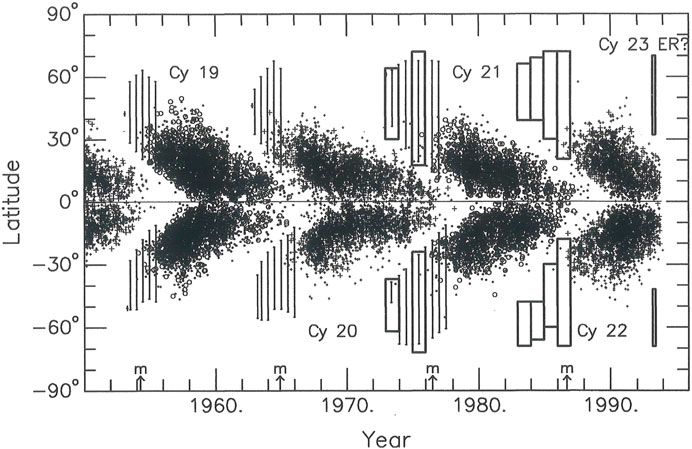
FIGURE 6. Butterfly diagrams of active regions with sunspots. Regions with sunspot areas >100 millionths of a hemisphere are shown alternately for successive cycles by + signs and small circles. The rectangular boxes indicate the latitude range of ephemeral regions with a preferential orientation reversed from lower-latitude regions. The light vertical bars represent small Ca II plage regions which are ephemeral regions seen in that spectral line. The last sunspot region belonging to a cycle is shown by a small circle superposed on a + sign. The times of solar minima (m) are shown as vertical arrows on the bottom line of the horizontal axis (credit: Figure 9 in Harvey, K. L. (1994) with permission to reproduce from Springer-Verlag).

FIGURE 7

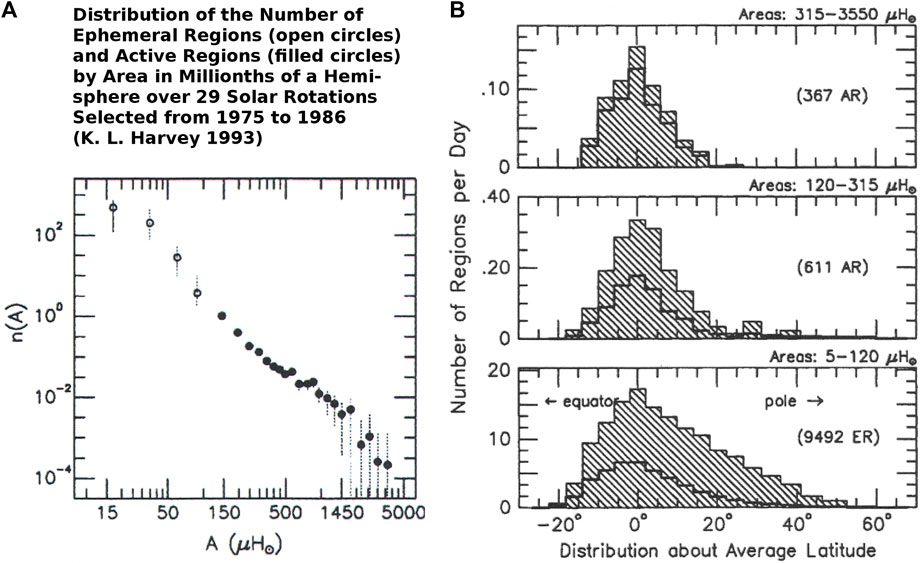
FIGURE 7. (A) This distribution shows that ephemeral active regions (open circles) fit smoothly into the same power law distribution as active regions (filled circles). (B) These graphs compare the populations of three sizes of active regions as shown in the upper right in millionths of a solar hemisphere. This panel illustrates the inverse relationship between the numbers of active regions and their areas; the larger the area, the smaller are their numbers, and conversely, the smaller the areas, the larger are their numbers. It also shows that all sizes of active regions over a solar cycle have their maximum number at the same average latitude. It confirms that the ephemeral regions constitute the largest fraction of the population of active regions (credit: Harvey, 1993a; Figure 5, with permission to reproduce from Springer-Verlag).

Further thought should also be given to the pyramid-shaped graphs in Figure 7B. Harvey (1993a) shows that the populations of the active regions of all sizes are centered around the same average latitudes. It is surprising that there is little evidence of a second peak at the higher latitudes although the shape of the distribution is asymmetric in the sense of having higher numbers at the higher latitudes where one might expect to see more evidence of the high latitude band of active regions with opposite east-to-west or west-to east bipolar magnetic orientations. Future studies of ephemeral active regions should seek to verify whether there is or is not a distinct minimum in the latitude distribution of the active regions whose average orientations differ by approximately 180°. The suggestion is to test whether the polarity reversal is inherent in the population of the apparent bands of active regions (as now assumed), or whether the polarity reversal could be acquired as active regions develop.

It should be noticed that the scales of the three graphs in Figure 7B are each different, in order to show them in an illustration of convenient size for publication. The scale of the bottom graph, with the ephemeral active region population, is two orders of magnitude greater than the top graph showing the population of large active regions. A graph on a linear instead of a logarithmic scale would be more effective in showing the importance of the large population of ephemeral active regions compared to the small population of active regions with sunspots.

As a loose analogy, the population of ephemeral active regions is like a mountain of sand and little rocks. The variable population of sunspots is like the seasonal snows on the peak of the mountain. Sunspots, like snow, have different physical characteristics than the whole mountain; they only appear when the conditions are favorable. Before and after the cool sunspots begin to appear, only the “sand and rocks” of the active regions are present—but, it is the snow that first captures our attention.

More than any other individual’s research work, K. L. Harvey’s research for her PhD thesis (1993 a,b) was the unseen harbinger of the paradigm shift discussed in detail in the next section.

In further investigating the extended solar cycle, McIntosh et al. (2014) recognized that EUV bright points could be useful proxies for ephemeral regions. This was reasonable because many EUV bright points occur when one magnetic pole of an ephemeral region collides with a patch of opposite polarity.

It is not expected that all observable small brightenings match one-to-one with ephemeral regions. Some of the brightenings might or might not be miniature solar flares. Like tiny flares, the EUV bright points occur where magnetic features of opposite polarity collide but there could be more than one bright point or flare per ephemeral region, and ephemeral regions that are not associated with any bright points. Furthermore, ephemeral regions are not the only possible source of new magnetic fields. Little clumps of intranetwork magnetic flux can be another source of opposite polarity magnetic field which collides with network fields and result in bright points. Thus, there should be no expectation for an exact one-to-one relationship between the numbers of ephemeral regions and bright points. Despite these questions about how well EUV bright points serve as proxies for ephemeral regions, the high latitude band of tiny EUV bright events appears to be a practical and meaningful representation of ephemeral regions at high latitudes.

We also should keep in mind there is no evidence that the smallest of the active region population has been detected to date. It is a reasonable speculation that magnetograms of higher spatial resolution over the whole solar disk will become available in the future.

5 The recognition and ramifications of two complete 22-year Hale Solar Cycles

Using the EUV bright points as proxies for ephemeral regions, McIntosh et al. (2014) showed, the Sun has two complete 22-year solar cycles present continuously. Each 22-year cycle exists in its own separate band of latitudes and has oppositely oriented bipolar magnetic fields from the previous cycle. Each cycle is a full 22 years, and a fraction more, in duration.

Arriving at 22 years via observations was significant because any shorter duration does not complete a cycle in time or space according to the definition of a cycle. As shown by Leamon et al. (2019), a true cycle is continuous; it does not have stops and starts. The beginning of every 22-year cycle is the same point in time as the end of the previous cycle. In this strict sense, the “sunspot cycle” is not a cycle. The occurrence of sunspots is a phase within a cycle rather than a true longer cycle by itself.

The findings of McIntosh et al. (2014) were amplified and extended in a series of articles (McIntosh and Leamon, 2015; Srivastava et al., 2018; Leamon et al., 2019; Leamon et al. 2020a; Leamon et al. 2020b; Leamon et al. 2020b; McIntosh et al., 2021; McIntosh et al., 2022). Together these research results dramatically revise our conception of solar cycles. Their work establishes the existence of at least six distinct properties of the two 22-year cycles that together overturn and replace the former concept of 11-year solar cycles. These properties, each seen in Figure 8, are stated below in more detail:

(1) Two 22-year solar cycles are present on the Sun continuously, instead of a single series of approximate 11-year cycles; this means there is no 11-year solar cycle; there is only a phase within each 22-year cycle in which a small fraction of active regions develop sufficient concentrations of magnetic flux to form sunspots.

(2) Each 22-year cycle consistently has its own west-to-east or east-to-west orientation of most of its bipolar active regions; there is no flipping of the dominant orientation of its active regions by 180° after the 22-year cycle begins.

(3) Each 22-year cycle begins at approximately 55° in latitude, not at lower latitudes.

(4) Each 22-year cycle continuously drifts toward the equator (as in the previous paradigm) but over 22 years instead of 11 years in each hemisphere.

(5) Every 11 years, a new 22-year solar cycle begins at high latitudes with the opposite west-to-east or east-to-west orientations of its active regions from those in the preceding cycle.

(6) When one cycle of active regions reaches the equator, the next cycle of active regions of the same polarity orientations of its active regions begins in a band of latitudes centered at approximately 55° that might be as wide as 30°. It is surmised that there is no gap in time between the end of a 22-year cycle of one polarity orientation close to the equator and the beginning of the next cycle with the same polarity orientation at approximately 55° in latitude. In other words, there is no breaking or interruption in successive cycles.

FIGURE 8

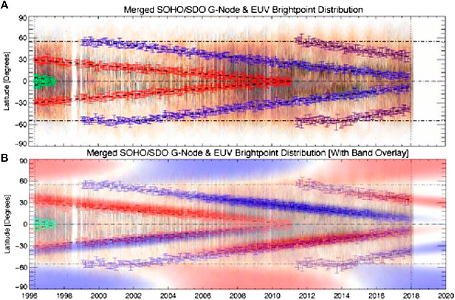
FIGURE 8. (A) Merged components of proxies, ephemeral regions, and active regions for solar cycle 22 in green, 23 in red, 24 in blue, and nearly half of cycle 25 in purple. Every solar cycle of active regions is represented by a chevron of 22 years duration and overlaps the preceding and following cycles by 11 years. Due to this overlap, consistent evidence of some part of the two separate cycles is present on the Sun at all times. This figure from Srivastava et al. (2018) adds color to chevrons whose width is a Gaussian distribution 10° wide in latitude. This approach to displaying the solar cycle data was used for showing the coronal bright points originally studied by McIntosh et al. (2014). Narrow bands of color are superposed to distinguish separate solar cycles. (B) A smoothed version of (A) with the dominant polarities of the polar regions also shown in alternate red and blue representing the positive and negative fields, respectively. The average polar fields alternate in polarity every 11 years consistent with a new solar cycle beginning in a new high latitude band every 11 years. In the active region latitudes, the northern hemispheric half of a chevron in the odd-numbered cycles are red in the sunspot zone; in the southern hemispheric half of the same chevron, the sunspot zone is blue. The main characteristics of the new paradigm: a) every solar cycle, represented by a chevron, is 22 years in duration; b) every 22-year solar cycle overlaps the preceding and following cycles by 11 years; c) every solar cycle begins at high latitudes in both hemispheres when the previous solar cycle, of the same polarity orientation, ends at the solar equator; d) successive new solar active regions, south of 55° in latitude, gradually appear closer to the solar equator over a 22-year interval (credit: Srivastava et al., 2018, Figure 3).

Properties in common with the former concept of 11-year solar cycles are

(a) The active regions of solar cycles exist in separate bands of latitudes not shared with the previous or following cycles.

(b) The change in the polarity of the network magnetic fields in the whole solar polar regions occurs around the time of the sunspot maximum, and 22 years are required for a complete cycle of magnetic fields in the polar regions.

(c) The change in the polarity of the polar fields is related to the largest active regions, not the whole population of active regions (Howard, 1992; Harvey, 1994). Multiple polarity changes can occur, but a main reversal in the dominant polarity occurs around the time of the solar maximum.

(d) The statistical properties of active regions within their belts of latitude are the same as previously known.

Figure 8A shows bright point proxies, ephemeral regions, and active regions for solar cycles 23 and 24 and nearly half of cycle 25. Cycle 23 is shown in red, cycle 24 in blue, and cycle 25 in a mixture of red and blue representing purple. The current solar cycle (25) has been present for 10 years at the time of this writing.

Figure 8B is a smoothed version of Figure 8A. The color-coding is changed to show polarity by color for positive-to-negative (west-to-east) polarities of active regions in the northern hemisphere (red) and negative-to-positive (east-to-west) polarities in the southern hemisphere (blue). This figure from Srivastava et al. (2018) superposes narrow bands of color on top of real data points. This attempt to emphasize the chevron patterns that represent each solar cycle tends to obscure the real data.

In Figure 8, at high latitudes, the polar fields are schematically represented as blue for the dominant positive polarity and red for the dominant negative polarity. Above approximately 55°, the background network magnetic fields gradually drift poleward. The continued action of differential rotation on filaments and filament channels gradually turns them nearly parallel with lines of constant latitude above approximately 55°. Some of the trailing polarity magnetic fields of the active regions move poleward faster than equatorward. At the same time magnetic flux above 55° gradually disappears due to photospheric magnetic reconnection. As it moves poleward. Eventually all of the previous polarity disappears in the polar region and is replaced by along the polarity boundary the opposite polarity field moving poleward. This change of polarity has been interpreted as signaling the beginning of “the next solar cycle.” However, in the new paradigm, the new cycle begins closely in time to the end of the previous 22-year cycle having the same polarity (Leamon et al., 2020a; Leamon et al., 2020b).

The lower panel is a smoothed version of the upper panel with the dominant polarities of the polar regions also shown in alternate red and blue, representing the positive and negative fields, respectively. The average polar fields alternate in polarity every 11 years consistent with a new solar cycle, having the opposite polarity, and beginning in a new high latitude band every 11 years. In the active region latitudes, the northern hemispheric half of a chevron in the odd-numbered cycles are red in the sunspot zone; in the southern hemispheric half of the same chevron, the sunspot zone is blue. This pattern is opposite in the even-numbered cycles. The main characteristics of the new paradigm are: a) Every solar cycle, represented by a chevron, is 22 years in duration. b) Every 22-year solar cycle overlaps the preceding and following cycles by 11 years. c) Every solar cycle begins at high latitudes in both hemispheres when the previous solar cycle of the same polarity orientation ends at the solar equator. d) Successive new solar active regions, south of 55° in latitude, gradually appear closer to the solar equator over a 22-year interval (credit: Srivastava et al., 2018, Figure 3).

Figure 9 (Altrock, 1997) has a similar chevron pattern for the green coronal line at 5303 A but is for cycles 20, 21, and 22. The green line serves as a proxy for the early phase of the 22-year cycles at high latitudes where ephemeral regions are difficult to detect. The end of cycle 20 occurs at approximately the end of 1978 with the last ephemeral regions of that cycle close to the equator. This same year is the beginning of cycle 22 at high latitudes as revealed by the green line emission. This provides an excellent example of the concept of terminators analyzed by Leamon et al. (2018), Leamon et al. (2019), Leamon et al. (2020b).

FIGURE 9

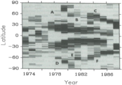
FIGURE 9. These chevrons represent the green coronal line emission for the end of solar cycle 20, most of cycle 21, a part of cycle 22, and the start of cycle 23 at high latitudes in 1985. The green line emission is a clearer signal of the beginning of the 22-year cycles than the tiny ephemeral region at high latitudes. However, the ephemeral regions near the equator are the clearest signal of the end of solar cycles. Combining information from both sets of data confirms the duration of 22 years as the fundamental length of solar cycles (credit: Altrock, 1988; also republished in Figure 13 by Harvey, 1992).

Active regions that developed sunspots were 10% of the total population of active regions and ephemeral active regions analyzed by Harvey (1994). Without the ability to recognize a lower limit for the size or duration of ephemeral regions in current-day magnetograms, it is only known that the percentage of the population of all active regions with sunspots is much less than 10%.

The reduced emphasis on the sunspot phase that comes with more complete knowledge of 22-year solar cycles, also affects how we see the Maunder Minimum and other long-term Grand Solar Minima. The Maunder Minimum of approximately 70 years with few or no consecutive sunspots is only approximately three and a quarter 22-year cycles. The greater precision of 22-year solar cycles, over the concept of variable 11-year solar cycles, is a strong confirmation of the deductions of Beer et al. (1998) and McIntosh et al. (2014) who have suggested that solar cycles continued with few or no sunspots during the Grand Solar Minima. McIntosh et al. (2014) further proposed that evolution into and out of a Grand Minimum is feasible with changes in the spatial overlapping of cycles; the more the overlap, the less the spots and vice versa. This could happen if the migration rates to lower latitudes increase and produce less overlap or decrease and result in more overlap of the bands of activity, without changing the overall 22-year rhythm of the solar cycle.

Twenty-two years is again emphasized here because it is a significant threshold to meet for the theory of the duration of solar cycles. At this limit, more precisely 22.2 years, solar cycles are continuous in both polarity bands in each hemisphere without any gap between the end of one cycle at the equator and the beginning of the next cycle of the same polarity at approximately 55° in latitude. Successive cycles broken by gaps imply a stop and start mechanism while continuous repeating cycles indicate a continuous mechanism behind solar cycles. The overlapping of two cycles out of phase by half a cycle reinforces the concept of continuity of the 22-year cycles. If any longer than 22.2 years, the diagrams in Figure 8 show that there would be spatial interference with the next cycle’s of magnetic fields with opposite polarity. In principle, the extended cycle concept comes to an end at 22.2 years. While this seems logical, it should be more thoroughly tested with observational data.

Leamon et al. (2018, Leamon et al., 2019, Leamon et al. 2020a, Leamon et al. 2020b) introduce the concept of a “terminator event,” a time when solar cycles disappear at the equator concurrent with the appearance of the next 22-year solar cycle at approximately 55°. This concept meshes usefully into the magnetic cycle (Hale, Ellerman, Nicholson and Joy, 1919; Hale and Nicholson, 1925). It confirms the duration of 22 years as the fundamental length of solar cycles instead of approximately 11 years.

As discussed in McIntosh and Leamon (2017), the existence of two solar cycles on the Sun for a long duration does not preclude the possibility of the Sun (or a star) in the past or future from having three solar cycles or more concurrently present over a longer or shorter interval of time than its present cycle.

Leamon et al. (2019) and Srivastava et al. (2018) further proposed that the end of a solar cycle, a termination point at the equator, and the beginning of the next solar cycle at high latitudes are causally linked in time. They showed that this linkage of the end and beginning of successive 22-year solar cycles could be as short as a single average 27-day rotation of the Sun. The finding of substantially greater precision in the recurrence of the 22-year cycle offers unprecedented possibilities for predicting future solar cycles and harmonics of the 22-year cycles.

The findings on solar cycles described herein have already been said to establish a new paradigm in the understanding of solar cycles (Srivastava et al., 2018). Previously, the 11-year solar cycle was regarded as the most fundamental cycle of all solar cycles. The longer 22-year cycle was thought to be due only to the 180° change in magnetic orientation of active regions and their sunspots near the beginning of each 11-year sunspot cycle. The new paradigm is consistent with seeing that the 22-year solar cycle is a more precise and fundamental “Hale Solar Cycle.”

In hindsight, we can see that the former concept of 11-year solar cycles is an illusion that was created by thinking that active regions with sunspots were the only significant active regions on the Sun. A single linear series of these sunspots was inadvertently created by plotting only the sunspot phase of every 22-year solar cycles as a single linear series in both butterfly diagrams and linear plots of sunspot number versus time. This was done under the assumption that only a linear series existed. The vast numbers of active regions without sunspots were not known, surmised, or theoretically predicted. Four decades (1973–2014) of studies identified as “the extended solar cycle” gradually brought increasing evidence that these two assumptions were not true as demonstrated by McIntosh et al. (2014).

Again, in hindsight, the apparent change in magnetic polarity between each approximate 11-year sunspot cycle is due to the lack of recognizing the full, 11-year overlap in time of any two successive 22-year solar cycles that are always simultaneously present. In the old paradigm, we skipped back and forth between the sunspot phase of the two 22-year cycles and called that “the solar cycle.” By inadvertently skipping from the sunspot half of a 22-year cycle to the sunspot half of the next 22-year cycle, it appeared as if an abrupt reversal of the orientation of active regions had taken place. Now, it is clear there is no abrupt change in polarity at the beginning of the sunspot cycle because the previous solar cycle has been present for 6–8 years. The previous paradigm was a type of illusion resulting from not yet including ephemeral active regions as playing a significant role in solar cycles. This, in turn, should not be regarded as human error; it was a natural conclusion from not yet having magnetograms of sufficiently high resolution to adequately detect the ephemeral active regions.

A more subtle point to mention is that 22-year cycles are more symmetric in time around the solar maximum than mentioned in the previous paradigm when the sunspot phase was synonymous with the concept of solar cycles. The rise of the sunspot phase of the cycle is well known to occur 3–4 years before the solar maximum and the decay phase to last 7–8 years after the solar maximum. By contrast, the whole solar cycle that includes the ephemeral regions tends to begin closer to 11 years before the solar maximum and to continue for 11 years after the solar maximum. This difference in the timing of the sunspot phase might be related to the observed fact that sunspots tend to grow larger and last longer after the solar maximum than before it. This is when the active region belt is centered closer to the equator. In addition, only a few complete 22-year cycles have been documented. Uncertainty remains about whether the sunspot number, the traditional way of determining the solar maximum, coincides with the maximum in the total magnetic flux of solar cycles.

6 The roles of ephemeral active regions and elementary bipoles in solar cycles

The change in the role of ephemeral active regions from insignificant to significant is one of the biggest upside–down turns in the new paradigm for solar cycles (Srivastava et al., 2018). For the understanding of solar cycles, ephemeral regions have emerged from trivial features to essential. As illustrated in Figure 8, ephemeral regions define the beginning, middle, and ending phases of the 22-year solar cycle (McIntosh et al., 2021). They are the primary means of tracing the early phase of the Hale Solar Cycle for at least 7–8 years before sunspots appear, and to continue during the late phase for 3–4 years after sunspots are no longer present (McIntosh et al., 2014). Furthermore, the greater the number of ephemeral regions, the greater the sunspot numbers (Harvey, 1994). Their vast numbers during the sunspot phase of the solar cycle (Harvey and Harvey, 1973; Harvey, 1993a) indicate they could become the primary means of predicting the amplitude and timing of future solar cycles (Leamon et al., 2019; McIntosh et al., 2021). In addition, they might be useful for predicting the amplitude and timing of the sunspot phase within the 22-year solar cycles (Srivastava et al. (2018).

The question “are ephemeral regions a separate population of phenomena from active regions that form sunspots?” has already been addressed in Section 4 by citing the studies of Harvey (1993a), Harvey and Zwaan (1993b). The fact that this question is still being asked warrants emphasizing it a second time. The three answers shown by Harvey are among the first observations that should be brought to the attention of anyone learning about solar cycles. These questions and their answers are of sufficient importance to be included in proposals for a new generation of higher quality and higher resolution magnetograms from space. The requirement has not gone away for the “newer and better observations of small bipolar magnetic regions” that Babcock sought in his pursuit of the theory of solar cycles. Recognition of the previously unknown properties of the two 22-year solar cycles is now justification for continuing to pursue Babcock’s dream shared by the worldwide community of solar researchers.

With increasing observations of magnetic spot cycles on other stars, the understanding of solar cycles is more relevant than ever to the stellar cycle research community (Bondar and Katsova, 2020). It should be highly important to know that spot cycles on other stars might be accompanied by magnetic field components far beneath the highest resolution observations obtainable now. This would have bearing on interpreting Maunder Minimum–like intervals on Sun-like stars such as Eta Eridani (Metcalf et al., 2012). At the same time, the shallow depth of ephemeral regions makes observations of stellar surfaces more promising and intriguing.

A recent study of Kutsenko (2020) compares the rotation rates of ephemeral active regions and active regions. Kutsenko verifies the common understanding that the depths of ephemeral regions are shallower than larger active regions and originate within 0.98 solar radii of the photosphere.

The graphs of Harvey as shown in Figures 7A, B demonstrate the major point made in an article by Beer et al. (1998). During the “grand Solar Minima,” such as the famous Maunder Minimum (Eddy, 1976; Eddy, 1983), solar cycles are still expected to be present in the form of ephemeral regions when few or no sunspots are observed during these solar cycles. For further discussion on this topic, the readers are referred to McIntosh and Leamon (2015).

Although ephemeral regions are a major part of the solar cycles before, during, and after active regions develop sunspots, in another aspect of the solar cycle, they play no role. They do not play even a minor role in determining the polarity of the magnetic flux which reaches the poles. The articles of Harvey (1992, Harvey, 1994) call attention to the knowledge that ephemeral active regions and small active regions make no significant, long-term, net contribution to the network magnetic flux anywhere on the Sun. For small active regions, equal quantities of positive and negative magnetic flux disappear from the photosphere nearly in situ. Harvey concludes “… the net contribution of an ephemeral region to the unipolar fields is 0.”

Harvey (1994) along with Webb et al. (1984) and Makarov and Sivaraman 1989a, Makarov and Sivaraman 1989b) show that the well-known rapid migration of the polar crown filaments toward the solar poles begins in concert with the appearance of sunspots. The migration does not start earlier in the solar cycle. Harvey’s (1994) analysis reveals that the magnetic flux which reaches the polar regions, originates entirely or almost entirely from the largest active regions. Howard (1992) also argues that all unipolar large-scale magnetic patterns can be traced to the emergence of magnetic flux in active regions and nests of active regions. These articles also confirm that ephemeral regions have little or no importance in which magnetic flux reaches the poles.

These results, in the two paragraphs above, have led to a sharp contrast in how ephemeral regions and large active region contribute to the observed properties of solar cycles in very different ways.

A recent article on small bipoles in the polar regions by Jin et al. (2020) describes events they called “bipolar magnetic emergence.” They were found at latitudes above 60° north and south of the equator. I treat these as ephemeral active regions because the authors have provided no information that justifies any separate designation. The significance of their study was finding over 300 such ephemeral active regions from the combination of observations of both the north and south polar regions. Some of the ephemeral active regions produced brightening events at 211 Å from the Atmospheric Imaging Assembly (AIA) during the year from June 2010 to May 2011. An important result was finding that the ephemeral regions in the polar areas have random orientations. The randomness of their orientations is not evidence that these small bipoles in the polar regions are not a component of solar cycles. A relatively large fraction of ephemeral regions in the active region belts also do not develop the west-to-east or east-to-west orientations of major active regions (Harvey, 1992; 1994).

The above result of Jin et al. (2020) is complementary to the findings of Tlatov et al. (2010) who separated ephemeral active regions into two groups. They called the smaller group Quiet Sun Regions (QSRs) and the larger ones Ephemeral Regions (ERs). Because their study relied on their program to identify bipoles, the smallest category was subject to including random background noise. However, Tlatov et al. (2010) found that the ER showed a preference in orientation depending on the polarity of the large-scale magnetic fields around and overlying the ephemeral regions. This statistical result is complementary to that of Jin et al. (2020). In the polar regions above 60° in latitude, there are no closed large-scale fields for ephemeral regions to align with. All magnetic reconnections send particles straight into the solar wind. Together, these two separate studies are consistent with the idea that most ephemeral regions have an overlying large-scale field to keep them from having random orientations. In any case, we should expect continuous interaction between newly emerging magnetic fields and any source of large-scale magnetic fields in which they emerge. An exception might be rare ephemeral regions that emerge already aligned with their local environmental magnetic field.

Chae et al. (2001) studied ephemeral regions around a large quiescent filament with the usual and essential overlying canopy of coronal loops. The spine of the tall filament that they studied is almost parallel with the polarity boundary at the photosphere except at the ends where the filament threads can splay to a wider pattern. The tall barbs curve from the spine to the chromosphere but are not resolved except near their footpoints. Because this is a tall, dextral, quiescent filament in the northern hemisphere, the angle of the barbs along the sides of the spine would be large and close to perpendicular (approximately 75–85°) to the long axis of the filament spine.

The filament erupted during the second day of the 5 days of observations and was recorded and analyzed. The filament spine, its barbs, and the overlying loops might have been already slowly rising and changing for hours to days preceding the eruption.

Chae et al. (2001) found a dominant direction for the ephemeral regions that did not apply to all of the ephemeral regions in the environment of the large quiescent filament. The dominant direction was similar to that of a cluster of ephemeral regions near the spine of the filament. That dominant direction did not match any specific features or direction that they thought could be related to ephemeral regions. However, in their Figure 1, as they had noted, the dominant orientation of the ephemeral regions was closer to being opposite to that of the magnetic field of the coronal loops overlying the filament than to any other feature of the whole erupting system. Being opposite in direction to the overlying loops means that the direction of the magnetic field in the barbs was inverse. It is now well known that the field direction in all barbs is inverse because the barb footpoints along the sides of the spine are small magnetic features opposite in polarity to the network magnetic fields on each side of the filament spine (Martin et al., 1994). The inverse magnetic field of the component of the filament magnetic fields perpendicular to the spine of the filament was first established for the vast majority of filaments by Leroy (1978). In their early observations of the filaments, the threads of the spine and barbs were not spatially resolved. Hence, the reason for the inverse magnetic field component perpendicular to the spine was a major puzzle for at least 1.5 decades.

Chae et al. (2001) did not offer any definitive explanation for this preferred direction of the bipoles. However, they did not consider whether the ephemeral regions could be aligned with the barbs of the filament before or during their eruption. The magnetic field in the barbs of filaments are along their threads and that direction is close to being opposite to the direction of the overlying loops. Therefore, the dominant direction of the ephemeral region bipoles would be more closely aligned with the inverse direction of the filament barbs than any other feature. It should be remembered that this filament erupted after the first day of their observations when the magnetic field environment of the new ephemeral regions might have been in a major state of change.

More studies like that of Chae et al. (2001) should be done to see if in other cases, there is any evidence that ephemeral regions close to the spine could align with the inverse magnetic field of the barbs.

To date, the spatial resolution of full-disk magnetograms has not yet been high enough to determine if there is a lower limit to the area or magnetic flux of ephemeral active regions. The graphs in Section 4 by Harvey (1993a), conservatively reveal that the population of ephemeral regions is 90% of the total population of all active regions. However, the real percentage of the total population must be more than 90% because many ephemeral regions are more short-lived than 1 day and therefore not seen and counted in daily magnetograms. Magnetograms of high spatial resolution also reveal many new active regions forming in existing active regions.

The pattern of formation of ephemeral regions has been compared by Harvey et al. (1975) and Martin (1990) with the way the larger active regions develop. They were found to be the same. This is further substantial evidence that ephemeral active regions and larger active regions with sunspots belong to the same population of solar features. Both are formed from pairs of tiny knots of magnetic field herein called “elementary bipoles.” The remainder of this section is devoted to clarifying the observed properties of elementary bipoles. They are the basic units of magnetic flux from which the active regions of solar cycles are observed to originate. At this point in our studies, ephemeral regions and elementary bipoles are the same manifestation of new emerging magnetic flux. An example of a large number elementary bipoles spread unusually broadly is shown in Figure 10 from Strous and Zwaan (2001). Their bipolar nature is better seen in movies than in single images as shown in Figure 10.

FIGURE 10

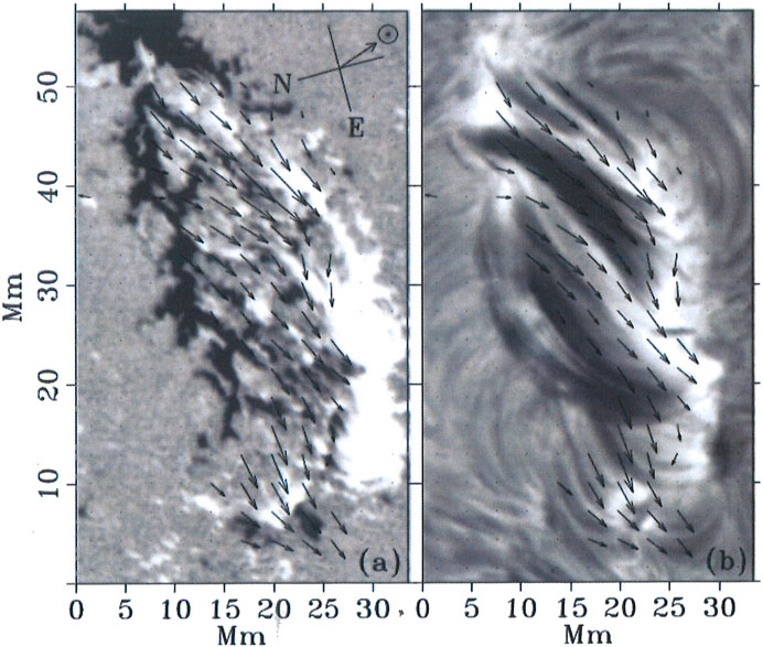
FIGURE 10. The image on the left is a line-of-sight magnetogram showing tiny white (positive) and black (negative) elementary bipoles between the main opposite polarity magnetic fields of a large, newly emerging active region. The initial pairing of the positive and negative elementary bipoles is not evident in a single image but can be seen in a time-lapse movie of this active region. The overlaid arrows show the direction of the magnetic field from a vector magnetogram. The image on the right reveals dark arch filaments from an H-alpha image. The arches connect the little bipoles that have separated from each other and exist at the footpoints of the arches. In the image on the right, the dark spot in the lower right is a sunspot being created by the merging of positive elementary bipoles (credit: Strous and Zwaan, 1999, Figure 6; by courtesy of L. Strous).

Vrabec (1974) was the first to acquire and show observations of sufficiently high quality, during intervals of good seeing, to clearly see streams of tiny bipoles, no larger than 2 arc seconds in diameter. He displayed them in movies made from a series of magnetograms taken at the San Fernando Observatory. He observed tiny bipoles successively separating into knots of opposite polarity. These knots of single polarity flowed in opposite directions to the sites where they coalesced and formed sunspots. He called the pattern of magnetic knots “MFIs” for “moving flows inward” meaning “into sunspots.” He also saw moving flows outward, MFOs, from sunspots. The latter were the well-known radial outflows in the moats around sunspots first studied by Harvey and Harvey (1973) from the magnetograms taken at the Kitt Peak National Observatory. The speeds of the MFIs are comparable to MFOs. However, in MFIs, the dot-like positive and negative poles move directly away from each other, the same as in ephemeral active regions. In MFOs, the pairs of opposite polarity dots move in the same radial direction outward from the sunspot penumbrae without separating widely from each other.

Vrabec’s observations revealed that sunspots were a second stage of magnetic flux increase initiated separate from the sites of emergence of the stream of very small-scale bipoles at the photosphere.

In H-alpha images, elementary bipoles are identifiable by the arch filament systems that are most clearly seen in H-alpha or calcium images (Bruzek, 1969; Frazier, 1972a).

Several high-resolution observations (of MFIs) were published after those of Vrabec (1974). However, the authors and peer reviewers did not initially recall or realize they were the same features that Vrabec had identified as MFIs. Martin (1990) called them “elementary bipoles,” Strous and Zwaan (1999) identified them as “flux emergence events” and Bernasconi et al. (2002) used the name “moving dipolar features (MDFs).” All of these high-resolution observations revealed their role in forming sunspots in the same way as those recorded by Vrabec (1974).

Sunspot formation required exceeding a threshold of magnetic flux in the coalescing bipoles. This was evident from the number of elementary bipoles that streamed from the site of emergence because they appeared to have the same small size of 1–2 arc seconds in diameter found by Vrabec (1974). This separate process of sunspot formation was identified as “convective collapse” described by Zwaan (1978) and Spruit (1979). If there are not enough elementary bipoles, or they are not driven together with enough force, sunspots do not form. Instead, these elementary bipoles either cancel and disappear, when their separate poles collide with magnetic fields of opposite polarity, or they merge to form the remaining parts of the magnetic fields of active regions, or both at the same time (Martin, 1990). The evidence to date is that all active regions are built from one or more elementary bipoles, which is consistent with Martin (1990) calling them “the building blocks of active regions.”

Martin (1990) made a selective study of elementary bipoles observed from birth at the Big Bear Solar Observatory using the former video magnetograph and H-alpha images under conditions of good seeing. Martin chose examples observed from the smallest active regions with a few elementary bipoles to successively larger ones with tens of elementary bipoles from three different sites. The following properties were reported in Martin (1990):

(1) Elementary bipoles are distinct and a characteristic sign of new magnetic flux appearing in both ephemeral active regions and active regions.

(2) The individual positive and negative elementary poles are usually detectable for tens of minutes to a few hours but there are large variations in their observable lifetimes due to interactions with neighboring elementary bipoles as well as to observing conditions and to instrumental sensitivity.

(3) In its simplest, earliest, and smallest form, a single active region is an elementary bipole that consists of only one positive and one negative juxtaposed magnetic knots that continuously move in opposite directions from their initial site. The separation speed is higher than other motions on the quiet Sun. Their separation speed is an essential identifier. Otherwise, basic elementary bipoles would be endlessly confused with small canceling magnetic features.

(4) If one of the poles of an elementary bipole collides with another magnetic feature of opposite polarity, it becomes a part of a canceling magnetic feature. A canceling magnetic feature is one in which equal and opposite polarity magnetic fields are disappearing along their common boundary. Due to canceling and merging, elementary bipoles have relatively short lifetimes from minutes to a few hours.

(5) Ephemeral regions that are larger than one elementary bipole often consist of a cluster of elementary bipoles developing within a few minutes of one another. Their motions can be parallel or in random directions from one another. Ones that are parallel or nearly parallel to each other will merge, combine their fluxes, and will then no longer be identifiable as elementary bipoles.

(6) The elementary bipoles can be seen before the arch filaments form above them in the chromosphere and low corona.

No fundamental difference has been found between elementary poles of short-lived ephemeral regions and active regions with sunspots (Martin, 1990). Many elementary bipoles cancel or merge with other elementary bipoles and become the other parts of active regions around their sunspots. The magnetic flux of elementary bipoles was estimated to be in the range of 200–600 Gauss (Martinez-Pillet et al. (1998).

Large active regions often form from multiple sites of elementary bipoles within or adjacent to a new active region (Martin, 1990). An example of a large number of elementary bipoles in a major new active region is shown in Figure 9 from Strous and Zwaan (1999). The spread of the elementary bipoles is much more extensive than in most active regions studied by Martin (1990). This is not surprising because many different centers of elementary bipoles can develop in medium and large active regions. For examples published to date, there is large variation in the number of clusters that form and in the direction they spread.

High-resolution, limited-field observations show that all active regions and their sunspots are built from elementary bipoles. Because the bipoles are not individually larger than a single ephemeral active region, Martin (2018) suggested all active regions might be surface phenomena which develop increased depth where their magnetic flux is highly concentrated.

The idea that sunspots are shallow phenomena forming at the photosphere and then extending to greater depths is consistent with the toroidal flows that develop as sunspots grow. They tend to become nearly round and symmetric if the magnetic fields of their associated active regions are simple and bipolar rather than complex. Such a large number of research articles have been written about sunspot formation, it is common knowledge that sunspots have downflows in their umbrae and upflows near the edges of their penumbrae throughout their lifetimes. The developed pattern of flows becomes like a toroid completely inside the surrounding sunspot moat where moving magnetic features flow outward. This inner toroidal part of the flows within sunspots is incompatible with merging into the pattern of rising intranetwork magnetic fields where Frazier (1972a, Frazier (1972b) suggested they form. Instead, the pattern of inner, downward toroidal flows is consistent with their formation at the boundaries of and vertices of supergranules where downflows occur as observed and studied by Born (1974) and subsequently by many other authors.

Martin (2018) concluded that this cited collection of observations was strong evidence for sunspots growing wider and deeper as long as their site was fed by elementary bipoles, and convective collapse could continue. The observations are consistent and there is no known contradictory observational evidence to concluding that sunspots are shallow and develop from the photosphere and downward to greater depths (Martin, 2018).

Substantial evidence has been cited that ephemeral regions are shallow (Kutsenko (2020), that most sunspots are shallow (Martin, 2018), and that active regions form from tiny elementary bipoles no larger than ephemeral active regions (Vrabec 1974; Martin 1990, Strous and Zwaan (1999); Bernasconi et al., 2002). Because these observations show that essentially all active regions originate from small scale bipoles, it is reasonable to anticipate further findings confirming that the primary sources of new magnetic flux seen at the photosphere are shallow. Will we be looking more diligently in the future to the near-surface shear layer for a near-surface dynamo (Brandenburg, 2006), or even closer to the photosphere (Jarboe et al., 2017)? This shallow focus (Kutsenko, 2020) seems inescapable for theory to be relevant to the active region population consisting of two fundamental 22-year Hale Solar Cycles.

7 Candidate magnetic fields to replace the polar fields every 11 years

Observations over the whole Sun have shown that large areas of unipolar magnetic fields develop mostly from the spreading of the magnetic fields of active regions. Observations by Babcock and Babcock (1955, 1958) show that this diffusion of the magnetic fields results in systematically putting opposite polarities of magnetic fields in the two polar regions. Most fascinating has been Babcock’s discovery that the polar fields gradually reverse polarity during the maximum of each sunspot cycle. The polar field disappears and is replaced by unipolar fields of the opposite polarity. Learning how these reversals take place has been a long-enduring observational and modeling problem. Significant results have been achieved.

Differential rotation and the random walk of the network of magnetic fields are two of the main processes that have been proven to result in the redistribution of the magnetic fields of active regions over the whole Sun (Wang et al., 1989; 1991). Meridional circulation, although slow, was shown to be another relevant factor (Wang and Sheeley, 1994). The role of the random walk caused by solar convection was modeled by Leighton (1964).

The solar cycle theories of Babcock (1961) and Leighton (1969) initiate and develop the concept that the tilt of active regions with respect to the solar equator is the main factor in determining the magnetic fields that reach the poles. For this reason, numerous articles have been written on the statistical properties of the tilt of active regions. This role has been included in recent reviews (Cliver, 2014; Hathaway, 2015; Weber et al., 2023). There is no need to reiterate the role of tilt in this review.

It should be mentioned here that the topic of flux cancellation has been introduced into the modeling of the transport of magnetic flux as an assumption. Cancellation was not included in the solar cycle theories of Babcock (1961) or Leighton (1969) except it was assumed that was how the polar fields disappeared. Now cancellation is mentioned in an off-hand way as a means of also eliminating magnetic flux from opposite hemispheres at the solar equator (Petrie, 2022 and references therein). With the thoroughness of the modeling of strong and weak magnetic flux (Petrie, 2022), the global aspects of the solar cycle seem to be thoroughly observed and modeled.

Observationally, however, there are still questions about the details of how the transfer of magnetic flux takes place from the active region belt to the polar regions. The merging and cancellation, discussed in Section 3, obscures the identity of specific sources of magnetic fields in relatively short intervals of time from hours to a few days. Under these circumstances, tracking and maintaining the identity of all sources of change is exceedingly difficult.

A current requirement is to recognize additional important observational factors, probably some not known to Babcock or Leighton, which affect magnetic field migration. A question not often addressed sufficiently is, why does the random walk not result in a continuous mixing of opposite polarity network and intranetwork magnetic fields? Differential rotation and meridional circulation would contribute only a bit more, if any, to the mixing of opposite polarities. As the active regions visibly spread over time, new active regions continuously develop within the older spread-out remnants. This factor contributes significantly to the mixing of opposite polarity magnetic fields. Additionally, the population of the small ephemeral active regions is large and broadly distributed over the whole Sun, which includes the polar regions (Jin et al., 2020). Furthermore, tiny intranetwork magnetic fields that depart from their convection cells by flowing into the lanes between supergranules. They are yet another source of mixing of opposite polarity magnetic fields. In the narrow lanes between supergranules, small intranetwork magnetic fields are observed to interact with any encountered magnetic feature of opposite polarity occupying the same lane. With all three of these large factors contributing simultaneously to the mixing of magnetic fields of opposite polarity (Martin, 1988). What are the opposing factors that create the unipolar network magnetic fields? How do unipolar areas of network magnetic fields sustain and increase in area over time?

Observationally, the answer is straightforward. Two solar plasma rules that apply to the line-of-sight component of magnetic fields on the Sun are now well known. These are:

(a) When opposite polarities come in contact, they are observed to cancel (Livi et al., 1985; Martin et al., 1985; Martin, 1998, and hundreds of subsequent articles by other authors). “Cancel” in the cited articles means only that equal amounts of positive and negative magnetic fields are observed to disappear at a common boundary between them (Martin, 1988; Martin, 1990). This is an observational definition; not a proposed mechanism on how magnetic flux disappears.

(b) When the same polarity features migrate into contact, they are observed to merge without any loss in magnetic flux (Martin et al., 1985; Livi et al., 1985, and numerous other previous and subsequent articles that mention this factor).

The ubiquity of canceling magnetic features was recognized first from video magnetograms taken at the Big Bear Solar Observatory. This does not imply that the observed flux loss from the photosphere was not previously observed and considered seriously, especially at sites where solar flares occurred.

The Big Bear video magnetograms were unique at that time because the observer could select the integration time of pairs of images acquired at the video rate (15 frames per second for each pair of the two polarities acquired sequentially). The integration of 1,024 video pairs was especially good for enhancing the visibility of the magnetic fields on the “quiet” Sun, which was then revealed to be highly dynamic. These observations were not very popular because the active region magnetic fields were saturated beyond any practical use. After magnetograms from the Solar Dynamics Observatory became available, numerous studies included observations of canceling magnetic fields.

The interpretation of cancellation, that best fits the observations, was established to be magnetic reconnection at or very close to the photosphere (Litvinenko and Martin, 1999; Litvinenko and Martin, 1999; Litvinenko et al., 2007). There are other interpretations, such as submergence of the canceling magnetic fields from the top of the photosphere to an unknown depth beneath the photosphere. Differing interpretations are the reason for keeping observational definitions and their interpretations separate and clear.

Evidence that magnetic reconnection in canceling magnetic features occurs very close to or at the photosphere is:

(1) the lack of any sudden brightening in the chromosphere or corona concurrent with the disappearance of both polarities of the magnetic field

(2) downflows in the photosphere observed at cancellation sites

(3) concurrent transverse flows observed in the chromosphere simultaneously with the downflows in (2) above.

The disappearance of the line-of-sight component of the magnetic field is evidence that the magnetic field has changed configuration to such an extent that its line-of-sight component is no longer being observed. Where does the disappearing magnetic field find a new residence? Some authors have provided evidence that all or part of the magnetic field becomes submerged below the photosphere (Harvey et al. XXXX). However, concurrent transverse flows (3 above) are also invariably found along the polarity boundaries in the chromosphere emanating from the sites of reconnection at the photosphere. These simultaneous downflows and outflows (2 and 3), away from observable sites of cancellation, are strong evidence of magnetic reconnection versus complete submergence. These flows are the initial dynamics of filament channel formation along boundaries between opposite polarity magnetic field components (Livi et al., 1985; Martin et al., 2012; Martin, 2015). Filaments are not sustained when the cancellation ceases (example in Litvinenko and Martin, 1999). Further confirming the association between canceling magnetic fields and filament formation, (Wood and Martens, 2003) have shown that the magnetic flux that developed during the formation of a filament is roughly equivalent to the magnetic flux that disappeared during the associated cancellation beneath the forming filament.

While cancellation is correlated with many types of solar features and events in different ways, the relationship of cancellation to magnetic field migration is the aspect relevant to this review.

When cancellation occurs [magnetic field rule (a) mentioned above], the migration of the magnetic fields, due to the random walk, is quickly reduced to the slow speed of the observed disappearance.

Filament channels and filaments occur only along boundaries between areas of opposite polarities where magnetic fields are canceling (Martin et al., 1985; Martin et al., 1994). They are major markers of where the local slowing of the random walk occurs, but not the reason why the migration nearly stops.

Anderson and Martin (2005) have shown canceling magnetic fields along filament channels effectively retard the intermingling of magnetic network flux of opposite polarity. The network magnetic fields of either polarity can only move along narrow boundaries between supergranules (Martin, 1994). A single cancellation of two fragments of opposite polarity magnetic fields is sufficient to block one lane. The lanes on average are roughly 30 Mm apart, the average diameter of supergranules. They encircle all convection cells but the flows along the lanes are temporarily interrupted at the vertices between cells. A few cancellation sites are sufficient to block migration across a filament channel 100 Mm in length. Tens of canceling magnetic fields are all that is required to block all intermingling of opposite polarity magnetic fields over a filament channel several hundreds of megameters in length. This is why cancellation is the dominant observed factor in keeping areas of opposite polarity network magnetic fields from mixing across filament channels throughout the quiet Sun and in active regions.

Cancellation along polarity boundaries is the primary dynamic that increases and sustains areas of unipolar network magnetic fields that originate from new bipolar active regions. In these ways, filament channels are the gate keepers of flux migration. The emphasis here is on filament channels rather than filaments because filament channel formation, related to cancellation, does not stop when the filaments, above their filament channels, erupt with CMEs.

The plasma magnetic field rule (b), merging of same polarity features, plays a role more often recognized as assisting in the sustaining and increasing of the area of unipolar magnetic fields. Mergers, like canceling magnetic fields, occur between magnetic fields of the same polarity irrespective of their origin (Martin, 1988). Common examples of mergers are observed among the elementary bipoles within growing active regions between one pole of ephemeral regions and network magnetic fields. They are observed in moving magnetic features after they flow away from developed sunspots (Rust, 1968; Harvey and Harvey, 1973). The dynamics of merging is simply the joining of areas of the same polarity until the initially separate fields of the same polarity are no longer identifiable as separate features. Quantitatively, a merger is the sum of two or more observed fragments of magnetic field before they merge. Areas of single polarity network magnetic fields away from filaments are places where the magnetic field migration, due to transport by random walk, is operating at its best.

Although mergers help maintain and increase areas of unipolar network magnetic fields, they are not permanent. If the splitting apart of same polarity network fields did not also occur, the random walk, driven mostly by convection, might not occur. It is observed that clumpiness of network magnetic fields is related to network fields dwelling temporarily at the vertices between supergranules. These bits of magnetic flux are caused to move again, by forces associated with growth of new convection cells or other dynamics of new or old active regions of all sizes.

While canceling sites nearly stop the local migration due to the random walk and block the intermingling of opposite polarity network magnetic fields, they do not stop differential rotation from acting on filament channels.

In active regions with east-to-west or west-to-east orientations, filaments and their channels are initially aligned nearly north-to-south or south-to-north but with local changes in the direction when new active regions form near them. Differential rotation gradually decreases the north-to-south and south-to-north component and increases the east-to-west or west-to-east components such that these filaments become diagonal features. These filaments, but not all filaments, develop southwest to northeast orientations in the northern hemisphere, and northwest to southeast orientations in the southern hemisphere.

If the filament channels survive the diagonal phase without disappearing or merging with other filament channels, they eventually become oriented nearly west-to-east or east-to-west, almost parallel with lines of constant latitude. This is most clearly seen on the poleward side of the active region belts. Filament channels and their canceling magnetic fields serve like shepherd dogs of differential rotation. As the channels move, they put up filaments as convenient flags of where magnetic fields are canceling along boundaries between opposite polarity magnetic fields. This enables us to record the higher contrast filaments, which over days to months and years, provide a record of where the channels have been. Filaments are not always benign flags revealing the changes ordered by differential rotation. They erupt frequently but new ones form in nearly the same locations as those that have erupted from their filament channels. Using the observations of filaments collected together from several observatories, Bocchini created an amazingly clear diagram revealing the two 22-year solar cycles on the Sun. This diagram adapted by Cliver (2014) is shown in Figure 11.

FIGURE 11

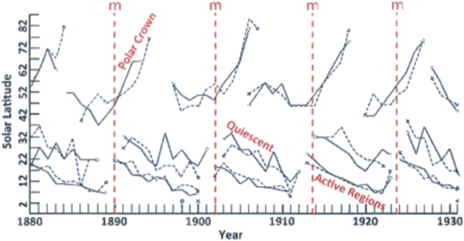
FIGURE 11. Two 22-year solar cycles are continuously evident in this presentation of filament data by Bocchino (1933). The 22-year patterns become clearer in mind if one overlooks the gaps representing the 11-year intervals that were formerly thought to be the duration of solar cycles. Two sets of filament tracks move equatorward every 11 years. The lower latitude track is an apparent continuation of the quiescent filament track during the preceding 11 years. This is evidence that filaments have retained the evidence of the two simultaneous solar cycles in separate latitude bands (Credit: from Cliver (2014) that was adapted from a figure in Bocchino (1933).

Solar cycles are more often represented by newly emerging flux rather than by filaments or filament channels that are commonly thought to be only related to decaying magnetic fields. Yet, the changing polar magnetic fields, related to the migration of filament channels, have long been known to have an important role in solar cycles (Leroy et al., 1983; Leroy, and Noens, 1983; Leroy, 1989).

Active regions show a tendency for their leading polarity to be closer to the equator than to their trailing polarity. This is known as “tilt.” Joy’s law is the tendency for tilt to increase with latitude and with decreasing magnetic flux in active regions. However, the scatter in tilt also increases with latitude as the average sizes of active regions decrease with latitude. Considering the many factors that affect the evolution of active regions, it is not clear why Joy’s law persists. Joy’s tendency is only a few degrees but it has been considered highly significant. It has been the topic of many statistical studies following Babcock’s (1961) and Leighton’s (1969) suggestions that the tilt is the main factor in why the trailing polarity is the one that first reaches the pole during every 11-year sunspot cycle.

Attributing significance to the tilt of the axis of bipolar active regions is puzzling. The lessening of tilt over time is an observed trend in major active regions (Weart, 1970). Additionally, the largest active regions show the least tilt. Moreover, Howard (1992) and Harvey (1994) have each shown that essentially all of the magnetic flux that reaches the solar polar regions is due to the largest active regions and complexes of active regions. Considering these observations, necessarily calls into question the assumption that tilt is the main factor in why the trailing polarity is the one that dominantly reaches the pole during every 11-year sunspot cycle.

An important result about filaments by Tang (1987) helps offer an alternative reason why a major portion of the trailing polarities of active regions reach the pole before the leading polarity. While it was already known that filaments can form along any boundary between opposite polarity magnetic fields (Babcock and Babcock, 1955; Smith et al., 1965; Tandberg-Hanssen, 1974), Tang (1987) study had revealed that twice as many filaments form at polarity boundaries between active regions than within the center of active regions between their two main areas of opposite polarity.

In continuing this explanation of selective magnetic field migration, we will call the filaments that form within active regions “W filaments” and those that form between active regions “B filaments.” This division of filaments into two main categories was already noted by Babcock and Babcock (1955), Smith et al., 1965) and Tandberg-Hanssen (1974). In the active region belts in each hemisphere and during periods of the formation of many new large active regions, there are often series of filaments in the middle of the active region belt alternating like: W B W B W B W B…. To be more specific, if we add the magnetic polarity designation of (+) for the western polarity, (−) for the eastern magnetic polarity in the northern hemisphere, the series of W and B filaments would look like −W + B −W + B − W + B − W + B ….

To develop, the B filaments can only form and become long-lived structures, when magnetic reconnection in the corona first connects some of the negative (−) trailing polarity magnetic fields of the active regions to the west with the (+) polarity of the active regions to the east. Then, the B fields can be represented more completely as +B− and the whole series can be represented as −W+ +B− −W+ +B− −W+ +B− −W+ +B− …. Relative to the W filaments, the (+) polarity is the leading or western polarity and (−) is the following or eastern polarity. But, relative to the B filaments, the (−) negative polarity is the leading or western polarity and the (+) polarity is the trailing or eastern polarity.

Differential rotation, in the northern hemisphere, acts on all of these magnetic fields such that W filaments and B filaments become diagonal. If north is up and west is to the right, and diagonal lines represent the filaments, the series can be depicted as −\+ +\− −\+ +\− −\+ +\− −\+ +\− …. This depiction should make it obvious that the B filaments have acquired their magnetic fields from some of the preceding and following active regions as they spread. It is commonly observed that the B filaments only form when the spreading of opposite polarity magnetic fields come in contact and begin canceling.

Relative to the W filaments in active regions in the northern hemisphere, differential rotation gradually adds a north–south component as indicated by the symbols (−\+). This tends to put the leading (+) polarity more to the north and the (−) polarity more toward the south in active regions in the northern hemisphere. However, we know from observations that it is the (−) polarity [not the (+) polarity] that first reaches the north pole for the sample solar cycle being represented here.

Next, we note the same effect of differential rotation acting on the B filaments that is represented by (+\−). In this case, differential rotation has pushed the (−) polarity more northward toward the pole and the (+) polarity more southward. Therefore, as differential rotation continues, the set of B filaments (+\−) are favored strongly to next contribute to the polar fields and the W filaments (−\+) might be the ones more likely to migrate toward the equator as shown in Figure 11. This preferential motion of a set of filaments toward the poles and two sets toward the equator are shown in the graph of long-term filament evolution in Figure 11 (Figure 6 in Cliver, 2014, which he adapted from Bocchino, 1933).

For the southern hemisphere, the entire pattern is reversed. Therefore, in the southern hemisphere, the next polarity reversal will result from differential rotation acting on the B filament channels and their surrounding fields in the same way as is for the northern hemisphere. This favors the (+) polarity fields to migrate toward the south pole as expected.

The choice of which polarity of magnetic fields arrives at the poles during every solar maximum is not as simple as described above. This is because some active regions develop roughly north or south of other active regions. In these cases, B filaments can form quickly with nearly east-to-west or west-to-east orientations. Differential rotation has little effect in changing the direction of these filament channels. However, these channels can slowly move toward areas of lower magnetic flux density. That direction is usually toward the poles. This shows that these filament channels can also be a determining factor in deciding which polarity reaches the poles first. The origin of subpolar crown filaments and their channels have to be studied to see how their channels quantitatively contribute to the role of herding specific polarity magnetic fields toward the poles. In the same hemisphere, some filament orientations would favor (+) magnetic flux reaching the poles in some solar circumstances and the (−) polarity magnetic fields in other circumstances. These filaments are consistent with our knowledge that one or more multiple polar reversals are sometimes observed before a main polarity is established in the polar regions.

An important mechanism of the formation of B filaments was first put forth by Hansen and Hansen (1975). They describe the formation of a nearly horizontal quiescent B filament, and its filament channel, forming between opposite polarity magnetic fields. They give the specific example of a new filament channel, and its filament, and its overlying coronal loop system forming between the polar magnetic field and the opposite polarity magnetic fields of one pole of an active region in the active region belt in the northern hemisphere. This is the same mechanism of formation of filament channels and filaments which applies to all B filaments. Physically, all filaments form by the same mechanisms (Martin et al., 2012). However, the solar circumstances, that precede and accompany their formation, are different for W filaments in active regions and B filaments that form between active regions.

The conclusion from the observations cited are

(1) It is unlikely that the tilt of active regions plays a significant role in determining what magnetic field is transported to the poles during the rise to solar maximum; differential rotation would tend to guide the leading polarity westward and poleward and the following polarity westward and southward. This would tend to effectively remove the tilt of active regions most commonly oriented east-to-west or west-to-east.

(2) Filament channels, that form under the coronal loop systems between large active regions (or decaying active regions), are the prime candidates for allowing differential rotation to guide them, and the newly associated part of the trailing polarity of the preceding active region, westward and poleward.

(3) In specific solar circumstances, poleward of the active region belts, other factors might determine, or contribute toward determining, which polarity will reach the poles, among these factors are: the action of canceling and merging of magnetic fields, filament formation, differential rotation, random walk, and meridional circulation. These circumstances could account for some cases in which the leading polarity migrates poleward instead of only the trailing polarity.

The qualitative picture, derived here from combining the results in published studies, requires verification. What is required in the future are more detailed quantitative studies of the evolution of solar magnetic fields than have yet been made or modeled. This especially includes the role of canceling magnetic fields, filament channel formation, and differential rotation. Such studies should be made over long intervals of time during the sunspot phase and the non-sunspot phase of the 22-year solar cycles.

The identity of the origin magnetic fields is lost rather quickly due to canceling and merging. It is highly desirable for studies to be done by visually identifying and tracking changes in addition to by attempting to follow the identity of magnetic features by computer programs alone. Models can be adjusted to appear to correctly fit a solar situation involving multiple parameters, even without including all of the essential observed parameters, such as canceling features. These can contribute to an observed pattern in some solar circumstances, and not in others.

8 Initiation of the polarity reversal of active regions at the beginning of 22-year Hale Solar Cycles

In this section, we explore the literature relevant to the question: why do active regions change polarity at the beginning of each 22-year solar cycle? One might first also ask, “are there any other phenomena in addition to active regions which reverse their west-to-east or east-to-west orientation every 11 years?”

In this author’s awareness, there is only one group of closely related phenomena that yields a positive answer to this question. Well-documented in the literature, these phenomena are polar crown filaments, subpolar crown filaments, and their filament channels (Rust, 1967; Leroy, 1978; Leroy et al., 1983; Bommier et al., 1985; Leroy, 1988; Martin, 1990; Bommier et al., 2021). Understanding how and why the polar crown filaments and subpolar crown filaments develop opposite east-to-west and west-to-east directions every 11 years requires at least a minimal understanding of both their evolution and the creation of the direction of the magnetic fields along filament channels and filaments.

In Figure 12, provided by V. Bommier, the several polar crown filaments in the northern hemisphere are along the polarity reversal boundary designated by the thin green line. This boundary was formerly often called “the neutral line” but the true meaning is that the magnetic field is horizontal along the polarity boundary. The red arrows represent the magnitudes and directions of the magnetic fields at a point on the filament at the base of the arrow. The arrows are in opposite directions in the polar crown filament and subpolar crown filaments. Specifically, in the northern hemisphere, the direction of the magnetic fields in the polar crown filaments are west-to-east and the subpolar crown filaments are east-to-west.

FIGURE 12

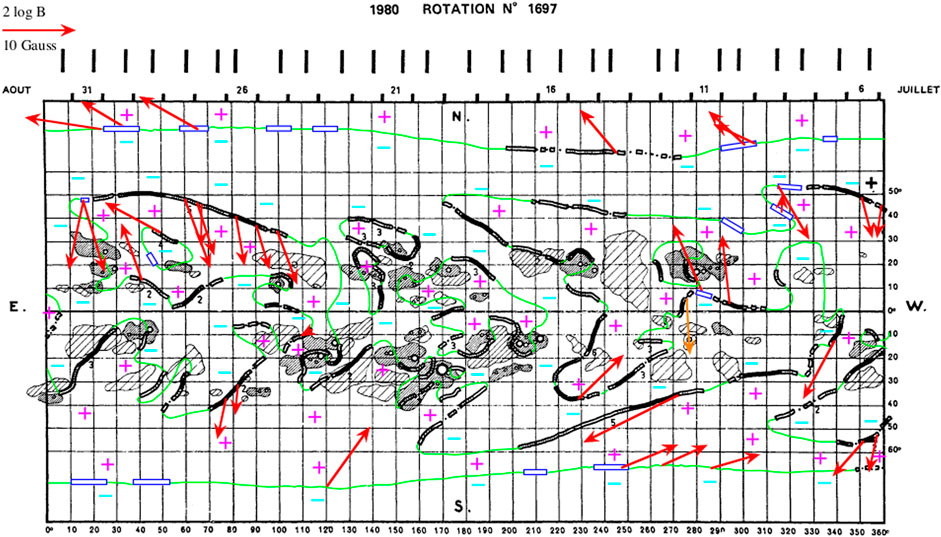
FIGURE 12. This synoptic chart of active regions and filaments for the whole of solar rotation no. 1697 is from the Meudon Solar Observatory. From right to left, the vertical lines above the map show the fraction of the central section of each full disk image which was incorporated into this chart. Photospheric magnetic fields are represented by red, + symbols for positive magnetic fields, and green − symbols for negative fields. These background polarities and the polarity boundaries (in green) have been added from McIntosh maps (NOAA/SEC) by Bommier et al. (2021) along with the red arrows which are proportional to the magnetic fields in the filaments. Polar crown filaments along the polar crown magnetic field boundaries in the northern and southern hemispheres are seen to be opposite in their west-to-east and east-to-west magnetic field directions. All of the arrows show the magnetic fields in the filaments are inverse. (They are in the − to + direction rather than + to − that is relative to the polarity of the major background fields on the two sides of each filament.) Along the next equatorward polarity boundary are the subpolar crown filaments which are opposite in their east-to-west or west-to-east direction from the polar crown filaments. The arrows on these charts were originally published in black and white by Bommier et al. (1985). (This updated color version was provided by the courtesy of V. Bommier and J. L. Leroy).

The opposing east-to-west or west-to-east directions of the polar crown and subpolar crown filaments were initially recognized in articles by Rust (1967), Leroy et al. (1983), Bommier et al. (1985), and Martin (1990). Reproduced in Figure 12 is a synoptic chart from the Meudon Observatory with the directions of the magnetic field superposed by Bommier et al. (2021). These synoptic charts refine and summarize the original work in Bommier et al. (1985) and references therein. Figure 12 shows the magnetic field directions for the polar crown and subpolar crown filaments for solar rotation no. 1697 (August 1980) during solar cycle 21.

The synoptic chart in Figure 12 is during the interval of increased rate of migration of the polar crown filaments toward the poles. The disappearance of the polar crown filament in the northern hemisphere occurred in the first half of 1981, shortly before the disappearance of the polar magnetic fields. The disappearance of the polar crown filaments is signified in Figure 13 by the change in polarity of the polar fields and in Figure 14 (Figure 5 from Harvey, 1994) by the curved lines representing the polar crown filaments and filament channels when they nearly reach the solar poles at 90° in latitude. They do not quite reach the pole before there is insufficient magnetic field to sustain them. Upon the complete disappearance of the polar crown filament, by definition, the subpolar crown filament is the new polar crown filament.

FIGURE 13

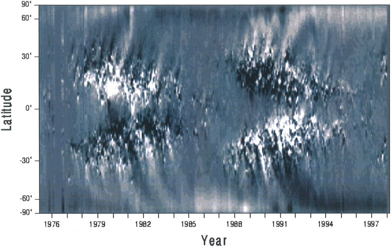
FIGURE 13. This butterfly diagram of magnetograms for solar cycle 21 shows the change of the polar field from positive to negative in the northern hemisphere and from negative to positive in the southern hemisphere in 1981. The northern hemisphere polar field remains negative until the next reversal to positive in 1991 during solar cycle 22. The southern hemisphere polar field reversed from positive to negative in 1990 (credit: Harvey, 1994, Figure 1, with permission from Springer-Verlag).

FIGURE 14

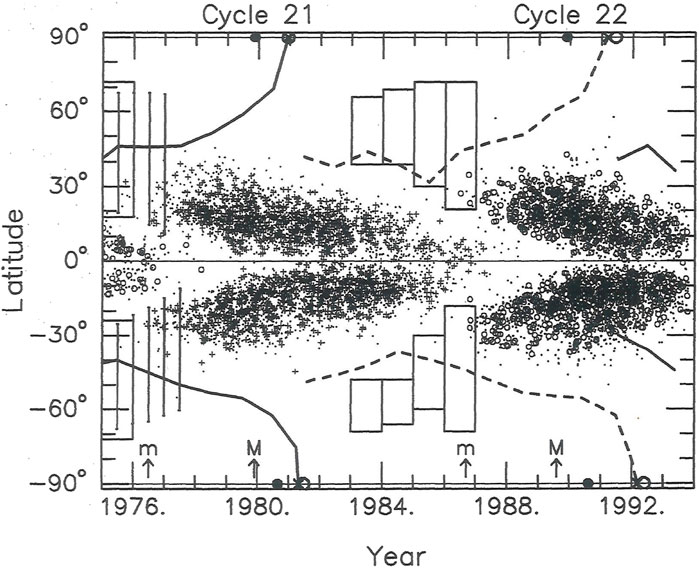
FIGURE 14. Butterfly diagram of sunspot regions of cycles 20, 21, and 22. The solid and dashed lines are the annual averages of the polarity inversion which represent the tracks of the polar crown filament for cycles 21 and 22. The latitude ranges of the high latitude belt of ephemeral active regions are shown as rectangles and small Ca II plage regions by vertical bars. Along the horizontal axis, ‘M’ is the time of solar maximum and ‘m’ is solar minimum (credit K. L. Harvey (1994) Figure 5, permission from Springer-Verlag).

The solar cycle reversal of the direction of the polar crown filaments around the time of the sunspot maximum has become especially well known since the early measurements of the horizontal component of the magnetic fields in polar and sub-polar crown filaments using the Hanle effect (Bommier and Leroy (1998).

This reversal in the direction of magnetic fields of the polar crown filaments is linked to the reversal of the polarity of the polar crown magnetic fields shown by Harvey (1994) in Figure 14 from synoptic charts of magnetograms for cycles 21 and 22. The reversals of the direction of the magnetic fields along filaments were also confirmed by Martin (1998) for cycles 21, 22, and 23. However, Martin (1990) used the chiral method of determining the direction of the magnetic field along filaments. That method required using the observed directions of barbs on filaments from H-alpha images, supported by the knowledge of the polarity of the photospheric magnetic fields on each side of the filament from magnetograms available at the Big Bear Solar Observatory. The chiral method is explained using many different examples in Martin et al. (2008). This method of determining the field direction along filaments was found to be consistent with the measurements of the magnetic field in filaments using the Hanle effect (Bommier and Leroy, 1998). That meant one can employ either method to extrapolate the alternating field directions along polar crown filaments for many solar cycles forward and backward in time.

Babcock and Babcock (1955) first demonstrated that filaments are markers of polarity boundaries. This led to recognizing that the alternating direction of the polar and subpolar crown filaments is due to the alternating bands of the decayed remnants of active regions that have evolved into north-to-south tiers in latitude (Leroy, 1978; Leroy et al., 1984; Bommier and Leroy, 1998). The solar cycle reversals of the direction of the magnetic field along filaments in both hemispheres are simply due to the poleward migration of alternating tiers of positive and negative magnetic fields at high latitudes that are well explained in Bommier et al. (2021).

The next questions are 1) is the west-to-east or east-to-west magnetic field direction of the ephemeral regions at the beginning of a 22-year solar cycle the same as that of the polar crown filament or the subpolar crown filament? 2) Does the band of new active regions at the beginning of a 22-year solar cycle spatially coincide with the polar crown or subpolar crown filament? The answers to these questions are also in published articles.

For the filaments:

A. Figure 12 (Figure 13 in Bommier et al. (1985)) shows the direction of the magnetic field of the polar crown filaments during August 1980, several months before they disappeared near the solar rotational poles. Their horizontal components are west-to-east for that time in solar cycle 21 and for all odd numbered cycles.

B. In Figure 5 by Harvey (1994), reproduced here in Figure 14, the west-to-east orientation applies to the polar crown filament in solar cycle 21 before its disappearance noted at the top of Harvey’s Figure 5. Therefore, the direction along the subpolar crown filaments in that cycle were east-to-west. That same subpolar crown filament is, by definition, the next polar crown filament (Figure 14 (Harvey’s Figure 5)). Therefore, the direction along the next polar crown filament in the northern hemisphere will be east-to-west for solar cycle 22 and for all even numbered cycles.

For the ephemeral regions:

As consistently observed, the polarity of the polar fields is always the same as the western polarity of the active regions in the same hemisphere and cycle. The polarity of the polar fields in the northern hemisphere, prior to the solar maximum in solar cycle 21, is positive as seen in Figure 13 (Figure 1 in Harvey, 1994). Therefore, active regions in the northern hemisphere in solar cycle 21 are oriented west-to-east according to the alternating pattern per solar cycle. Thus, the preferred direction of the ephemeral regions in the northern hemisphere in cycle 22 is the opposite; it is east to west.

Comparing these independently determined results for the orientations of polar crown filaments and ephemeral regions, the answer for the question above is: the magnetic fields of ephemeral active regions of a new solar cycle have the same preferred orientation as the polar crown filaments. In addition, in Figure 14, the latitude of the polar crown filament is approximately 45° in each hemisphere. This is slightly lower in latitude than the average latitude of 55° where the new 22-year solar cycles begin. However, the span of coronal arches above the polar crown filament can be 20° or more in width. It is the whole volume beneath the coronal loops that is relevant in this comparison. It is also important to notice that the polar crown filament is already established around the time of the emergence of the new active regions in the 22-year solar cycles.

The second question was “do the polar crown filaments and their channels coincide with the band of ephemeral regions at the beginning of a 22-year solar cycle?” The answer is in Figure 14 (Figure 5 in Harvey, 1994). The blocks represent ephemeral regions early in solar cycles 21 and 22. The curved line represents the track of the polar crown filaments and their filament channels. For approximately 3 or more years, the polar crown filament coincides with some part of the latitude bands of the new cycle ephemeral active regions.

With these correlations, established in the literature, between the polar crown filaments and ephemeral active regions in both space and time, it is reasonable to make a general hypothesis about how the polarity reversal of solar cycles are initiated:

Hypothesis. The apparent reversal of the orientation of ephemeral active regions at the start of every 22-year solar cycle is due to their aligning with the dominant east-to-west or west-to-east orientation of the filament channels and channel environment into which the ephemeral regions emerge. The alignment process is suggested to be magnetic reconnection.

The direction of the magnetic fields of the environment of filament channels and filaments varies significantly throughout the volume they occupy in the chromosphere and corona. This volume can include the varying directions of the magnetic fields of the coronal loop system over a filament and filament channel, the filament spine, the filament barbs, and the underlying photosphere. Therefore, substantial scatter in the direction of the ephemeral region magnetic fields should be expected to exist and depend on what part of the environment is the closest to the individual ephemeral regions at the time when the magnetic reconnections are taking place between it and the environmental magnetic fields.

This hypothesis is based on the observation that magnetic reconnection between magnetic fields, that are partially aligned, causes them to become more aligned.

Direct evidence favorable or unfavorable to this hypothesis is expected to be difficult to achieve due to the high latitude at which ephemeral active regions form early in 22-year solar cycles. Very high-resolution magnetograms and/or filtergrams are essential to determine the magnetic polarity information required about the ephemeral active region, such as their changes over time.

Searching for relationships between ephemeral regions and filaments and their filament channels at lower latitudes might lead to learning whether there is more evidence for or against the hypothesis. Such new studies could show a requirement to refine the hypothesis. New studies might also lead to asking new questions about what could cause a bias toward west-to-east or east-to-west orientations of active regions of any size.

This hypothesis should apply to not only ephemeral active regions during the start of a solar cycle but also to all active regions whose magnetic flux is initially less than that of the environmental magnetic fields into which the active region emerges.

Evidence in favor of the above hypothesis is shown in Figure 7 in the article by Tlatov et al. (2010). As stated above, large scatter in the orientation of both environmental magnetic fields of filaments and filament channels, and the orientations of the active regions, which emerge into the environmental magnetic fields, is expected. Therefore, statistical associations are not expected to be strong for ephemeral active regions. However, the degree of alignment should increase as the magnitude of the interacting magnetic fields increases.

A single statement summary of this section is the reversal of polarity of ephemeral regions at the beginning of each 22-year solar cycle is due to the reversed direction of the magnetic fields of the filament channel and environment of the channel into which they emerged. Reconnection between the ephemeral region magnetic fields and its environmental magnetic fields results in increased alignment of the ephemeral region structure with the west-to-east or east-to-west direction of the magnetic field into which it emerges.

9 Discussion: the transition to a new paradigm for solar cycles

This review has been written during a transition to a new paradigm in how solar cycles are viewed. The former paradigm was centered on sunspots and continued with new observations of the active region magnetic fields that encompass sunspots. In the previous paradigm, solar cycles were linear successions of sunspot/active region cycles of approximately 11 years. Two 11-year cycles were required for a complete magnetic cycle.

The slow transition to the new paradigm changed the focus from the sunspot belt to the global Sun. The emphasis switched from the 11-year sunspot cycle to the acknowledgment of the extended solar cycle. This recognition first depended on the new full-disk daily magnetograms at the Kitt Peak National Solar Observatory. They had sufficiently high spatial resolution to reveal vast numbers of small-scale active regions that did not reach a magnitude great enough to produce sunspots. Singly, these tiny active regions seemed insignificant; collectively, they have a colossal effect on how solar cycles are viewed. The magnetic flux they bring to the solar surface is greater than that in the active regions with sunspots. As if ephemeral regions are in control, their numbers increase early in each solar cycle. While continuing to increase their numbers, the ephemeral active regions begin to usher-in a lot of small active regions that produce small sunspots, followed by a lesser number of active regions with medium-area sunspots, and then a few active regions that produce large sunspots. After the solar maximum, for all sizes of active regions, the ephemeral active regions decrease their population but first they usher-out those active regions with sunspots approximately in reverse order to their ushering-in.

The culmination of the extended cycle is the recognition of two 22-year solar cycles present in separate latitude bands continuously. Two cycles each of 22 years duration are essential because each 22-year band of regions in latitude contains a dominance of west-to-east or east-to-west oriented active regions. The two cycles are offset by 11 years with the beginning of each 22-year cycle at the highest latitudes where the ephemeral active regions can be identified. The beginning of each 22-year cycle coincides with the disappearance of the polar magnetic fields of single polarity. These polar magnetic caps and the equator serve as markers of the hidden mechanism of the solar cycle clock. They mark the timing of the two 22-year cycles which are out of phase by 11 years with more precision than could be imagined earlier. The accuracy of this solar cycle clock is a harbinger of more accurate future predictions and offers new views of historical records.

Over the next decade, it is expected that the new paradigm will translate into new ideas, observations, and models for solar cycles. These will encompass observations yet to be fully understood about active regions. This will lead to greater understanding of their orientation patterns, peculiarities of their sunspots, tilts with respect to latitude and longitude, clustering in longitude, global polarity reversals, and depths of origin.

Notably, these key items for solar cycle research are almost the same as originally listed by Babcock (1961). In light of the new paradigm, they are echoes of Babcock’s research call, “Of particular value would be more and better measurements of the distribution and quantity of magnetic flux in BMR (bipolar magnetic regions) as a function of age.”

Now the little “bipolar magnetic regions” that bring on solar cycles are discussed as “ephemeral active regions” and “elementary bipoles.” As the progenitors of both larger active regions and their sunspots, what is their origin?

Author contributions

The author confirms being the sole contributor of this work and has approved it for publication.

Acknowledgments

The author expresses appreciation to Prof. Oddbjorn Engvold for reading and commenting on the scientific content of the manuscript, to Prof. Piet Martens for discussing the hypothesis for the initiation of polarity reversals at the beginning of 22-year solar cycles, to novelist Gil Roscoe and song-writer Alan Higgins for assistance in detailed editing of the manuscript, and to student Gabriel Higgins for resolving complications of fussy software.

Conflict of interest

The authors declare that the research was conducted in the absence of any commercial or financial relationships that could be construed as a potential conflict of interest.

Publisher’s note

All claims expressed in this article are solely those of the authors and do not necessarily represent those of their affiliated organizations, or those of the publisher, the editors, and the reviewers. Any product that may be evaluated in this article, or claim that may be made by its manufacturer, is not guaranteed or endorsed by the publisher.

References

Altrock, R. C. (1988). “Variation of solar coronal Fe XIV 5303 Å emission during solar cycle 21, in solar and stellar coronal structure and dynamics,” in Proceedings of the ninth Sacramento peak summer symposium, sunspot, NM. Editor R. C. Altrock (Sunspot, NM: National Solar Observatory), 414.

Google Scholar

Altrock, R. C. (1997). An 'extended solar cycle’ as observed in Fe XIV. Sol. Phys. 170, 411–423. doi:10.1023/a:1004958900477

CrossRef Full Text | Google Scholar

Anderson, M., and Martin, S. F. (2005). “Formation of an extraordinarily long filament channel,” in Large-scale Structures and their Role in Solar Activity, Proceedings of the Conference held, Sunspot, New Mexico, USA, 18-22 October, 2004. Editors K. Sankarasubramanian, M. Penn, and A. Pevtsov (IEEE), 201.

Google Scholar

Babcock, H. D. (1959). The Sun’s polar magnetic field. Astrophys. J. 130, 364. doi:10.1086/146726

CrossRef Full Text | Google Scholar

Babcock, H. D., and Babcock, H. W. (1955). The Sun's magnetic field 1952-1954. Astrophys. J. 121, 349. doi:10.1086/145994

CrossRef Full Text | Google Scholar

Babcock, H. D., and Babcock, H. W. (1958). “Photospheric magnetic fields,” in Electromagnet phenomena in cosmical physics. Editor bo lehnert, IAU symposium no. 6 (Cambridge: Cambridge University Press), 239–247.

CrossRef Full Text | Google Scholar

Babcock, H. D., and Livingston, W. C. (1958). National academy of Sciences: abstracts of papers presented at the annual meeting, 28-30 april 1958, Washington, D.C. Science 127, 1058–1063. doi:10.1126/science.127.3305.1058

PubMed Abstract | CrossRef Full Text | Google Scholar

Babcock, H. W. (1947). Zeeman Effect in stellar spectra. Astrophys. J. 105, 105B. doi:10.1086/144887

CrossRef Full Text | Google Scholar

Babcock, H. W. (1961). The topology of the Sun's magnetic field and the 22-year cycle. Astrophys. J. 133, 572. doi:10.1086/147060

CrossRef Full Text | Google Scholar

Babcock, H. W., and Babcock, H. D. (1952). Mapping the magnetic fields of the Sun. PASP 64, 282. doi:10.1086/126495

CrossRef Full Text | Google Scholar

Balasubramaniam, K. S., Pevtsov, A., and Rogers, J. (2004). Statistical properties of superpenumbral whorls around sunspots. Astrophys. J. 608, 1148–1155. doi:10.1086/420759

CrossRef Full Text | Google Scholar

Beer, J., Tobias, S., and Weiss, N. (1998). An active sun throughout the maunder minimum. Sol. Phys. 181, 237–249. doi:10.1023/a:1005026001784

CrossRef Full Text | Google Scholar

Bernasconi, P. N., Rust, D. M., and Geogoulis, M. K. (2002). Moving dipolar features in an emerging flux region. Solar Phys. 209, 119–139.

CrossRef Full Text | Google Scholar

Bocchino, G. (1933). Migrazione delle protuberanze durante il ciclo undecennale dell’attivata solare. Oss. Mem. Oss. Astrofus. Arcetri 51, 5–47.

Google Scholar

Bommier, V., Degl’Innocenti, E. L., Leroy, J.-L., et al. (1994). Complete determination of the magnetic field vector and of the electron density in 14 prominences from linear polarization measurements in HeI D3 and H alpha lines. Solar Phys. 154, 231–326.

CrossRef Full Text | Google Scholar

Bommier, V., and Leroy, J. L. (1998). Global pattern of the magnetic field vector above neutral lines from 1974 to 1982: Pic-du-Midi observations of prominences, New Perspectives in Solar Prominences, IAU Colloquium 167. Asp. Conf. Ser. 150, 434–438.

CrossRef Full Text | Google Scholar

Bommier, V., Leroy, J. L., and Sahal- Brechot, S. (1985). “MSFC workshop: measurements of solar fields, huntsville,”, Alabama, USA, 15-18 May, 1984. Editor M. J. Hagyard (NASA Conference Publication), 375.2374.

Google Scholar

Bommier, V., Leroy, J.-L., and Sahal-Brechot, S. (2021). 24 synoptic maps of average magnetic field in 296 prominences measured by the Hanle effect during the ascending phase of Solar Cycle 21. Astron. & Astrophys 647, A60. Id. A60. doi:10.1051/0004-6361/202038868

CrossRef Full Text | Google Scholar

Bondar, N. I., and Katsova, M. M. (2020). Long-term activity in photospheric low-mass stars with strong magnetic fields. arXiv:201.

Google Scholar

Born, R. (1974). First phase of active regions and their relation to the chromospheric network. Sol. Phys. 38, 127–131. doi:10.1007/bf00161830

CrossRef Full Text | Google Scholar

Brandenburg, A. (2006). “Location of the solar dynamo and near-surface shear,” in MHD theory and observations: a high resolution perspective. Editors H. Uitenbroek, J. Leibacher, and R. F. Stein (ASP Conference) 354, 121–126.

Google Scholar

Bray, R. J., and Loughhead, R. E. (1964). Sunspots. London: Chapman & Hall.

Google Scholar

Bruzek, A. (1969). Motions in arch filament systems. Sol. Phys. 8, 29–36. doi:10.1007/bf00150655

CrossRef Full Text | Google Scholar

Carrington, R. C. (1858). On the distribution of the solar spots in latitude since the beginning of the year 1854; with a map. MNRAS 19, 1–3. doi:10.1093/mnras/19.1.1a

CrossRef Full Text | Google Scholar

Chae, J., Martin, S. F., Yun, H. S., Kim, J., Lee, S., Goode, P. R., et al. (2001). Small magnetic bipoles emerging in a filament channel. Astrophys. J. 548, 497–507. doi:10.1086/318661

CrossRef Full Text | Google Scholar

Chatterjee, S., Hegde, M., Banerjee, D., Ravindra, B., and McIntosh, S. W. (2020).Time-latitude distribution of for 10 solar cycles: a study using Kodaikanal, Meudon, and Kanzelhohe data, Earth Space Sci., e00666, 7.

CrossRef Full Text | Google Scholar

Chian, A. C.-L., Rempel, E. L., Silva, S. S. A., Rubio, L. B., and Gosic, M. (2023). Intensification of magnetic field in merging magnetic flux tubes driven by supergranular vortical flows. MNRAS 518, 4930–4942. doi:10.1093/mnras/stac3352

CrossRef Full Text | Google Scholar

Cliver, E. W. (2014). The extended cycle of solar activity and the Sun’s 22-year magnetic cycle. Space Sci. Rev. 186, 169–189. doi:10.1007/s11214-014-0093-z

CrossRef Full Text | Google Scholar

Eddy, J. A. (1976). The maunder minimum. Science 192, 1189–1202. doi:10.1126/science.192.4245.1189

PubMed Abstract | CrossRef Full Text | Google Scholar

Eddy, J. A. (1983). The maunder minimum: a reappraisal. Sol. Phys. 89, 195–207. doi:10.1007/bf00211962

CrossRef Full Text | Google Scholar

Engvold, O., and Zirker, J. B. (2016). The parallel worlds of Christoph scheiner and Galileo galilei. Hist. Astron 7 (3), 332–345. doi:10.1177/0021828616662406

CrossRef Full Text | Google Scholar

Frazier, E. N. (1972a). The magnetic structure of arch filament systems. Sol. Phys. 26, 130–141. doi:10.1007/bf00155113

CrossRef Full Text | Google Scholar

Frazier, E. N. (1972b). The relations between chromospheric features and photospheric magnetic fields. Sol. Phys. 24, 98–112. doi:10.1007/bf00231086

CrossRef Full Text | Google Scholar

Hale, G. E. (1908). On the probable existence of a magnetic field in sunspots. Astrophys. J. 28, 315. doi:10.1086/141602

CrossRef Full Text | Google Scholar

Hale, G. E. (1913). Preliminary results of an attempt to detect the general magnetic field of the Sun. Astrophys. J. 38, 27–30. doi:10.1086/142013

CrossRef Full Text | Google Scholar

Hale, G. E., and Ellerman, F. (1918). The polarity of sunspots. PAAS 3, 81.

Google Scholar

Hale, G. E., Ellerman, F., Nicholson, S. B., and Joy, A. H. (1919). The magnetic polarity of sunspots. Astron. J. 49, 153–178. doi:10.1086/142452

CrossRef Full Text | Google Scholar

Hale, G. E., and Nicholson, S. B. (1925). The law of sunspot polarity. Astrophys. J. 62, 270–300. doi:10.1086/142933

CrossRef Full Text | Google Scholar

Hale, G. E., and Nicholson, S. B. (1938). Magnetic observations of sunspots, No. 498. Washington, D. C: Carnegie Inst. of Washington Publ.

Google Scholar

Hansen, S. F., and Hansen, R. T. (1975). Differential rotation and reconnection as basic causes of some coronal reorientations. Solar Phys. 44, 503–508.

CrossRef Full Text | Google Scholar

Harvey, K. (2000). Solar active regions: ephemeral, encyclopedia of Astronomy and astrophysics. Bristol: Institute of Physics Publishing. Available at http://eaa.iop.org/abstract/0333750888/2275.

Google Scholar

Harvey, K., and Martin, J. (1973). Observations of moving magnetic features near sunspots. Sol. Phys. 28, 61–71. doi:10.1007/bf00152912

CrossRef Full Text | Google Scholar

Harvey, K. L. (1992). The cyclic behavior of solar activity. Sol. Cycle ASP Conf. Ser. 27, 335–367.

Google Scholar

Harvey, K. L. (1993a). PhD thesis. University of Utrecht.

Google Scholar

Harvey, K. L. (1994). “The solar magnetic cycle,” in Solar surface magnetism (Kluwer: Kluwer Academic Publishers), 347–363.

CrossRef Full Text | Google Scholar

Harvey, K. L., Harvey, J. W., and Martin, S. F. (1975). Ephemeral active regions in 1970 and 1973. Sol. Phys. 40, 87–102. doi:10.1007/bf00183154

CrossRef Full Text | Google Scholar

Harvey, K. L., and Zwaan, C. (1993b). Properties and emergence patterns of bipolar active regions: I.Size distribution and emergence frequency. Sol. Phys. 148, 85–118. doi:10.1007/bf00675537

CrossRef Full Text | Google Scholar

Hathaway, D. H. (2015). The solar cycle. Sol. Phys. 7, 1. doi:10.12942/lrsp-2010-1

CrossRef Full Text | Google Scholar

Howard, R., and Labonte, B. J. (1980). The sun is observed to be a torsional oscillator with a period of 11 years. Astrophys. J. Part 2 - Lett. Ed. 239, L33–L36. doi:10.1086/183286

CrossRef Full Text | Google Scholar

Howard, R. F. (1992). On the large-scale distribution of solar magnetic fields. Sol. Cycle ASP Conf. 27, 44.

Google Scholar

Jarboe, T. R., Benedett, T. E., Everson, C. J., Hansen, A., Hossack, A. C., Morgan, K. D., et al. (2017). Evidence for a shallow thin magnetic structure and solar dynamo: the driver of torsional oscillations.

Google Scholar

Jiang, J., Cameron, R. H., and Schussler, M. (2015). The cause of the weak solar cycle. arXiv:1507.01764v1[Astro-ph.SR].

Google Scholar

Jiao, Q., Jiang, J., and Wang, Z.-F. (2021). Sunspot tilt angles revisited: dependence on the solar cycle strength. Astron. & Astrophys, 11615v1. arXiv:2106.

CrossRef Full Text | Google Scholar

Jin, C., Zhou, G., Zhang, Y., and Wang, J. (2020). The bipolar magnetic emergence in the solar polar region. Astrophys. J. Lett. 889, L26. doi:10.3847/2041-8213/ab65bf

CrossRef Full Text | Google Scholar

Kutsenko, A. S. (2020). The rotation rate of solar active and ephemeral regions – I. Dependence on morphology and peak magnetic flux. MNRAS 000, 5159–5166. doi:10.1093/mnras/staa3616

CrossRef Full Text | Google Scholar

Leamon, R. J., McIntosh, S. W., and Chapman, S. C. (2000a). The Hale cycle clock. Bristol, AGU Fall Meeting SH053.

Google Scholar

Leamon, R. J., McIntosh, S. W., and Marsh, D. R. (2018). Termination of solar cycles and correlated tropospheric variability. ADS. arXiv-prints.

Google Scholar

Leamon, R. J., McIntosh, S. W., and Title, A. M. (2020b). Deciphering solar magnetic activity: the solar cycle clock. Front. Astron. Space Sci. 9, 886670. doi:10.3389/fspas.2022.886670

CrossRef Full Text | Google Scholar

Leamon, R. J., McIntoshChapman, S. W. S. C., and Watkins, N. W. (2019). Timing terminators: forecasting sunspot cycle 25. arXiv.

Google Scholar

Leighton, R. B. (1964). Transport of magnetic fields on the Sun. Astrophys. J. 140, 1547–1562L. doi:10.1086/148058

CrossRef Full Text | Google Scholar

Leighton, R. B. (1969). A magneto-kinematic model of the solar cycle. Astrophys. J. 156, 1–26. doi:10.1086/149943

CrossRef Full Text | Google Scholar

Leighton, R. B., Noyes, R. W., and Simon, G. W. (1962). Velocity fields in the solar atmosphere. I. Preliminary Report. Astrophys. J. Let. 135, 474–499. doi:10.1086/147285

CrossRef Full Text | Google Scholar

Leroy, J.-L. (1978). On the orientation of magnetic fields in quiescent prominences. Astron. Astrophys. 64, 647–252.

Google Scholar

Leroy, J.-L. (1988). “Solar and stellar coronal structure and dynamics,” in Proceedings of the 9th Sacramento Peak Summer Symposium, Sunspot, New Mexico, 17–21 August 1987. Editor R. C. Altrock (IEEE), 422.

Google Scholar

Leroy, J.-L. (1989). “Dynamics and structure of quiescent solar prominences,” in Dynamics and structure of solar prominences. Editor E. R. Priest (Dordrecht: Kluwer Academic Publishers), 77.

Google Scholar

Leroy, J.-L., Bommier, V., and Sahal-Bréchot, S. (1983). The magnetic field in the prominences of thepolar crown. Sol. Phys. 83, 135.

CrossRef Full Text | Google Scholar

Leroy, J.-L., Bommier, V., and Sahal-Bréchot, S. (1984). New data on the structure of quiescent Prominences. Astron. Astrophys. 131-33.

Google Scholar

Leroy, J.-L., and Noens, J.-C. (1983). Does the solar activity cycle extend over more than an 11-year period? Astron. Astrophys. 120, L1–L2.

Google Scholar

Litvinenko, Y., Chae, J., and Park, S.-Y. (2007). Flux pile-up magnetic reconnection in the solar photosphere. Astrophys. J. 662, 1302–1308. doi:10.1086/518115

CrossRef Full Text | Google Scholar

Litvinenko, Y. E. (2010). Evolution of the axial magnetic field in solar filament channels. Astrophys. J. 720, 948–952. doi:10.1088/0004-637x/720/1/948

CrossRef Full Text | Google Scholar

Litvinenko, Y. E., and Martin, S. F. (1999). Photospheric magnetic reconnection and canceling magnetic features on the sun. Astrophys. J. 515, 435–440. doi:10.1086/307001

CrossRef Full Text | Google Scholar

Livi, S. H. B., Wang, J., and Martin, S. F. (1985). The cancellation of magnetic flux I - on the quiet Sun. Aust. J. Phys. 38, 855–873. doi:10.1071/ph850855

CrossRef Full Text | Google Scholar

Loughhead, R. E., and Bray, R. J. (1979). Sunspots. USA, Dover Publishers, Inc.

Google Scholar

Makarov, V. I., and Sivaraman, K. R. (1989a). Evolution of latitude zonal structure of the large-scale magnetic field in solar cycles. Sol. Phys. 119, 35–44. doi:10.1007/bf00146210

CrossRef Full Text | Google Scholar

Makarov, V. I., and Sivaraman, K. R. (1989b). New results concerning the global solar cycle. Sol. Phys. 123, 367–380. doi:10.1007/bf00149112

CrossRef Full Text | Google Scholar

Martin, S. F. (1988). The identification and interaction of network, intranetwork and ephemeral region magnetic fields. Solar Phys. 117, 243.

CrossRef Full Text | Google Scholar

Martin, S. F. (1990). Elementary bipoles of active regions and ephemeral active regions. Soc. Astron. Ital. Mem. 61, 293–315.

Google Scholar

Martin, S. F. (1998). Filament chirality: a link between fine-scale and global patterns new perspectives in solar prominences, iau colloquium 167. Asp. Conf. Ser. 150, 419–429.

CrossRef Full Text | Google Scholar

Martin, S. F. (2015). “The magnetic field structure in prominences from direct and indirect observations, Chapter 9,” in Solar prominences. Editors J.- C Vial, and O. Engvold (Germany: Springer Publishers), 205–235.

CrossRef Full Text | Google Scholar

Martin, S. F. (2018). Observational evidence of shallow origins for the magnetic fields of solar cycles. Front. Astron. Space Sci.Sec. Stellar Sol. Phys. 5, 315. doi:10.3389/fspas.2018.00017

CrossRef Full Text | Google Scholar

Martin, S. F., Bilimoria, R., and Tracadas, P. W. (1994). “Magnetic field configurations basic to filament channels and filaments,” in Solar surface magnetism. Editors R. J. Rutten, and C. J. Schrijver (Dordrecht: Kluwer Academic Publishers), 303.

CrossRef Full Text | Google Scholar

Martin, S. F., Engvold, O., and Lin, Y. (2008). A method of resolving the 180-degree ambiguity by employing the chirality of solar features. Sol. Phys. 250, 31–51. doi:10.1007/s11207-008-9194-8

CrossRef Full Text | Google Scholar

Martin, S. F., and Harvey, K. H. (1979). Ephemeral active regions during solar minimum. Sol. Phys. 64, 93–108. doi:10.1007/bf00151118

CrossRef Full Text | Google Scholar

Martin, S. F., Livi, S. H. B., and Wang, J. (1985). The cancellation of magnetic flux II - in a decaying active region. Aust. J. Phys. 38, 929–959. doi:10.1071/ph850929

CrossRef Full Text | Google Scholar

Martin, S. F., Panasenco, O., Berger, M. A., Engvold, O., Lin, Y., Pevtsov, A. A., et al. (2012). “The build-up to eruptive events viewed as the development of chiral systems, the Second ATST East Meeting: magnetic Fields from the Photosphere to the Corona,” in ASP Conference Series, San Francisco, 15 Dec 2012. Editors T. Rimmele, A. Tritschler, F. Woger, V. Collados, H. Socos Navarro, R. Schlichenmaieret al. (Astronomical Society of the Pacific), 157.463.

Google Scholar

Martinez-Pillet, V., Lites, B. W., and Skumanich, A. (1998). Vector magnetic fields of emerging solar flux, ESSP 417, 259–261.

Google Scholar

Mazumder, R. (2019). Properties of solar filaments in solar cycle 20-23 from McIntosh Archive. article id. 080.

Google Scholar

Mazumder, R., Chatterjee, S., Nandy, D., and Banerjee, D. (2021). Solar cycle evolution of filaments over a century: investigations with the Meudon and McIntosh hand-drawn archives. Astrophys. J. 919, 125. doi:10.3847/1538-4357/ac09f6

CrossRef Full Text | Google Scholar

McIntosh, S. W., and Leamon, R. J. (2015). Deciphering solar magnetic activity: on grand minima in solar activity, Front. Sol. Stellar Phys. article, Front. Astronomy Space Sci., Vol.2, 2, doi:10.3389/fspas.2015.00002

CrossRef Full Text | Google Scholar

McIntosh, S. W., and Leamon, R. J. (2017). Deciphering solar magnetic activity: spotting solar cycle 25. Front. Astron. Space Sci. 4, 4. doi:10.3389/fspas.2017.00004

CrossRef Full Text | Google Scholar

McIntosh, S. W., Leamon, R. J., Egeland, R., Dikpati, M., Altrock, R. C., Banerjee, D., et al. (2021). Deciphering solar magnetic activity: 140 years of the ‘extended solar cycle’ – mapping the Hale cycle. Solar Phys. 296, 89.

CrossRef Full Text | Google Scholar

McIntosh, S. W., Leamon, R. J., Egeland, R., Dikpati, M., Fan, Y., and Rempel, M. (2019). What the sudden death of solar cycles can tell us about the nature of the solar interior. Sol. Phys. 294, 88. doi:10.1007/s11207-019-1474-y

CrossRef Full Text | Google Scholar

McIntosh, S. W., Scherrer, P. H., Svalgaard, L., and Leamon, R. J. (2022). Uniting the Sun’s Hale magnetic cycle and “extended solar cycle” paradigms. Front. Astronomy Space Sci. 9, 923049. doi:10.3389/fspas.2022.923049

CrossRef Full Text | Google Scholar

McIntosh, S. W., Wang, X., Leamon, R. J., Davey, A. R., Howe, R., Krista, L. D., et al. (2014). Deciphering solar magnetic activity. I. On the relationship between the sunspot cycle and the evolution of small magnetic features. Astrophys. J. 792, 12. doi:10.1088/0004-637X/792/1/12

CrossRef Full Text | Google Scholar

Metcalf, T. S., Buccino, A. P., Brown, B. P., Mathur, S., Soderblom, D. R., Henry, T. J., et al. (2012). Magnetic activity cycles in the exoplanet host star Eta Eridani. arXiv:1212.4425v1 [astro-ph.SR].

Google Scholar

Munoz-Jaramillo, A., Benjamin, N., and Campusano, L. E. (2022). Solar anti-Hale bipolar magnetic regions: a distinct population with systematic properties. arXiv:2203.11898v1 [astro-ph.SR] 22 Mar 2022.

Google Scholar

Parker, E. N. (1955). The Formation of sunspots from the solar toroidal field. Astrophys. J. 121, 491–507. doi:10.1086/146010

CrossRef Full Text | Google Scholar

Parnell, C. E., DeForest, C. R., Hagenaar, H. J., Johnston, B. A., Lamb, D. A., and Welsch, B. T. (2009). A power-law distribution of solar magnetic fields over more than five decades in flux. Astrophys. J. 698, 75–82. doi:10.1088/0004-637x/698/1/75

CrossRef Full Text | Google Scholar

Pesnell, W. D. (2012). Solar cycle predictions (review). Sol. Phys. 281, 507–532.

Google Scholar

Petrie, G. (2022). Polar global magnetic field evolution and global flux transport. Germnay: Springer. doi:10.21203/rs.3.rs-2298525/v1

CrossRef Full Text | Google Scholar

Petrovay, K. (2010). Solar cycle prediction, living review. Sol. Phys. 17 (1). article id.2.

Google Scholar

Priyadarchi, A., Hegde, M., Jha, B. K., Chatterjee, S. M., Mandal, S., Chowdhury, M., et al. (2022). Detection of solar filaments using suncharts from Kodaikanal solar Observatory archive employing a clustering approach. arXiv:2212.12176v1 [astro-ph.SR].

Google Scholar

Richardson, R. S. (1941). The nature of solar hydrogen vortices. Astrophys. J. 41, 24. doi:10.1086/144238

CrossRef Full Text | Google Scholar

Robbrecht, E., Wang, Y.-M., Sheeley, , and Rich, N. B. (2010). On the ‘extended’ solar cycle in coronal emission. Astrophys. J. 716, 693–700. doi:10.1088/0004-637x/716/1/693

CrossRef Full Text | Google Scholar

Rust, D. (1967). Magnetic fields in quiescent solar prominences. I. Observations. Astrophys. J. 150, 313–326. doi:10.1086/149333

CrossRef Full Text | Google Scholar

Rust, D. M. (1968). in Structure and development of solar active regions, IAU symp. No. 35. Editor K. O. Kiepenheuer, 77.

CrossRef Full Text | Google Scholar

Rust, D. M., and Martin, S. F. (1994). “A Correlation between sunspot whirls and filament type,” in ASP Conf. Series Astron. Soc. Pacific, San Francisco, 3 September 1993. Editors K. S. Balasubramaniam, and G. W. Simon (IEEE), 337.

Google Scholar

Schwabe, M. (1844). Sonnenbeobachtungen im Jahre 1843. Von Herrn Hofrath Schwabe in Dessau. Astron. Nachrichten 21, 233.

Google Scholar

Simon, G. W., and Leighton, R. B. (1964). Velocity fields in the solar atmosphere. III. Large-scale motions, the chromospheric network, and magnetic fields. Astrophys. J. 140, 1120. doi:10.1086/148010

CrossRef Full Text | Google Scholar

Smith, S. F., Ramsey, H., and Howard, R. F. (1965). Some characteristic properties of solar magnetic fields. Astron. J. 70, 330. doi:10.1086/109605

CrossRef Full Text | Google Scholar

Snodgrass, H. B. (1987). Torsional oscillations and the solar cycle. Sol. Phys. 110, 35–49. doi:10.1007/bf00148200

CrossRef Full Text | Google Scholar

Spӧrer, G. (1894). Beobachtungen von sonnenflecken in den jahren 1885 bis 1893, Pub. Potsdam Obs. 10 (1), 3–147.

Google Scholar

Srivastava, A. K., McIntosh, S. W., Arge, N., Banerjee, D., Dipankar, G., Dikpati, M., et al. (2018). The extended solar cycle: muddying the waters of solar/stellar dynamo modeling or providing crucial observational constraints? Front. Astronomy Space Sci. Mini-Review 5. doi:10.3389/fspas.2018.00038

CrossRef Full Text | Google Scholar

Strous, L. H., and Zwaan, C. (1999). Phenomena in an emerging active region, II. Properties of the dynamic small-scale structure. Astrophys. J. 527, 435–444. doi:10.1086/308071

CrossRef Full Text | Google Scholar

Tandberg-Hanssen, E. (1974). Solar prominences. Dordrecht, Holland: D. Reidel Publishing C.

Google Scholar

Tandberg-Hanssen, E. (1995). The nature of solar prominences. Dordrecht: Kluwer Academic Publishers.

Google Scholar

Tang, F. (1987). Quiescent prominences – where are they formed?. Solar Phys. 107, 233.

CrossRef Full Text | Google Scholar

Tlatov, A. G. (1996). A model of the solar magnetic cycle with a meridian stream closed inside the convective zone. Quantum Electron 39, 794–798. doi:10.1007/bf02120957

CrossRef Full Text | Google Scholar

Tlatov, A. G., Makarov, M. I., and Sivaraman, K. R. (1989). New results concerning the global solar cycle, Sol. Phys. 123, 367, 380. doi:10.1007/bf00149112

CrossRef Full Text | Google Scholar

Tlatov, A. G., Vasil'eva, V. V., and Pevtsov, A. A. (2010). Distribution of magnetic bipoles on the Sun over three solar cycles. Astrophys. J. 717, 357–362. doi:10.1088/0004-637x/717/1/357

CrossRef Full Text | Google Scholar

Vial, J.-C., and Engvold, O. (2015). in Solar prominences. Editors J.-C. Vial, and O. Engvold (Switzerland: Springer International Publishing).

Google Scholar

Vrabec, D. (1974). “Streaming magnetic features near sunspots, chromospheric fine structure. Editor R. Grant Athay, IAU Symp. 56, Surfer's Paradise, Qld., Australia,” in 3-7 september 1973 (Dordrecht; Boston: Reidel), 201–231.

CrossRef Full Text | Google Scholar

Wang, H., and Li, H. (2022). Rediscovery of 23 historical records of naked-eye sunspot observations in AD 1618. Sol. Phys. 297, 127. Article 127. doi:10.1007/s11207-022-02046-w

CrossRef Full Text | Google Scholar

Wang, Y.-M., Nash, A. G., and Sheeley, N. R. (1989). Magnetic flux transport on the Sun. Science 249, 712–718. doi:10.1126/science.245.4919.712

PubMed Abstract | CrossRef Full Text | Google Scholar

Wang, Y. M., and Sheeley, N. R. (1994). The rotation of photospheric magnetic fields: a random walk transport model. Astrophys. J. 430, 399–412. doi:10.1086/174415

CrossRef Full Text | Google Scholar

Wang, Y.-M., Sheeley, N. R., and Nash, A. G. (1991). A new solar cycle model including meridional circulation. Astrophys. J. 383, 431–442. doi:10.1086/170800

CrossRef Full Text | Google Scholar

Weart, S. (1970). The birth and growth of sunspots. Astrophys. J. 162, 97–922.

CrossRef Full Text | Google Scholar

Webb, D. F., Davis, J. M., and McIntosh, P. S. (1984). Observations of the reappearance of polar coronal holes and the reversal of the polar magnetic field. Sol. Phys. 92, 109–132. doi:10.1007/bf00157239

CrossRef Full Text | Google Scholar

Weber, M., Schunker, H., Jouve, L., and Isik, E. (2023). Understanding active region origins and emergence on the sun and other cool stars. Space Sci. Rev. 219, 63. arXiv.2306.06536v1 [astro-ph.SR] 10 June 2023. doi:10.1007/s11214-023-01006-5

CrossRef Full Text | Google Scholar

Wilson, P. R., Altrock, R. C., Harvey, K. L., Martin, S. F., and Snodgrass, H. B. (1988). The extended solar activity cycle. Nature 333, 748–750. doi:10.1038/333748a0

CrossRef Full Text | Google Scholar

Wood, P., and Martens, P. (2003). Measurements of flux cancellation during filament formation. Sol. Phys. 218, 123–135. doi:10.1023/b:sola.0000013027.52104.c6

CrossRef Full Text | Google Scholar

Zwaan, C. (1978). On the appearance of magnetic flux in the solar photosphere. Sol. Phys. 60, 213–240. doi:10.1007/bf00156523

CrossRef Full Text | Google Scholar