Heliospheric 3-D MHD ENLIL simulations of multi-CME and multi-spacecraft events

1 Introduction

Numerical modeling plays a critical role in efforts to understand the connection between solar eruptive phenomena and their impacts in the near-Earth space environment and interplanetary space. Interpretation of remote observations and in-situ measurements, as well as reconstruction of three-dimensional (3D) structured and evolving solar wind (SW) together with propagating and interacting coronal mass ejections (CMEs), is a challenging task. This is even more challenging in the case of multi-CME events and multi-spacecraft observations. Multi-CME events are episodes when two or more CMEs interact with each other in the heliosphere, which is a common occurrence during times of maximum solar activity. Numerical simulations can provide global context, and they can help with the interpretation of observations. Modeling the origin of CMEs is still in the research phase,and real events are not expected to be routinely simulated in the near future (e.g., see reviews by Zhao and Dryer (2014); Riley et al. (2018); Vourlidas et al. (2019). Moreover, we cannot derive the 3D magnetic structure of CMEs from image data alone.

Therefore, we have developed the WSA-ENLIL-Cone modeling system, which uses remote observations of the photospheric magnetic field and white-light (WL) signatures of CMEs in coronagraphs to construct time-dependent boundary conditions at 21.5 Rs (0.1 AU) that drive the 3D numerical magnetohydrodynamic (MHD) code ENLIL (Odstrcil, 2003; Odstrcil et al., 2004a; Odstrcil et al., 2005). This “hybrid” modeling system enables the simulation of virtually any observed CME event as it propagates and interacts with the evolving background SW and interplanetary magnetic field (IMF) in the inner and mid heliosphere. The WSA-ENLIL-Cone modeling system ignores specifics of the magnetic eruption process; it takes the observed resulting structure and launches a hydrodynamic ejecta into the heliospheric computational domain to routinely predict heliospheric space weather, event-by-event, and much faster than in real-time.

Using hydrodynamic ejecta cannot predict (1) interactions involving CME magnetic structures (e.g., CME-solar wind, CME-CME); and (2) magnetic field components when the CME passes a planet or spacecraft (e.g., Bz component at Earth); This can be achieved by numerical MHD models that simulate either (1) coronal magnetic eruption (with subsequent heliospheric propagation) or (2) launch magnetic structures into the heliospheric computational domain. However, as mentioned above, the former is still in the research phase, and the latter simulates the propagation of various simplified magnetic-field structures (e.g., flux rope or spheromak). These structures are topologically different; they interact differently and require additional model-free parameters to fit observations. While these models are helpful in research studies, their application to operational predictions is severely hampered by the lack of magnetic field measurements needed to initialize the simulation.

The WSA-ENLIL-Cone model has proven to be reliable over the years for all observed CMEs in coronagraphs. Its accuracy in predicting the time of arrival (ToA) at Earth has been evaluated by various researchers (e.g., Taktakishvili et al., 2010; Riley et al., 2018; Wold et al., 2018). The ENLIL approach has also been adopted by the EUHFORIA (Pomoell and Poedts, 2018; Poedts et al., 2020) model. Recently, Mays et al. (2020) presented the Final Report from the NASA-NOAA project on evaluating the WSA-ENLIL-Cone model advancements for predicting the ToA at Earth. They used 38 CME events operationally fitted by SWPC forecasters and found that the prediction can be made with 6–8 h inaccuracy.

A stable and robust version of the ENLIL modeling system has been implemented at NASA Community Coordinated Modeling Center (CCMC), and it has served the heliospheric space weather community since 2005 (with over 8,300 user-requested runs by the end of 2022). Its operational version has been used daily by forecasters at NOAA/Space Weather Prediction Center (SWPC) since 2010 (Pizzo et al., 2011), UK MetOffice since 2014, and also at Korean Space Weather Center (KSWC), and Australian Space Weather Forecasting Center (ASWFC). NASA/CCMC also provides both mission science and space weather support to NASA heliospheric robotic missions and, within the recently established Moon to Mars (M2M) Space Weather Analysis Office (https://science.gsfc.nasa.gov/674/m2m/index.html), Also to human space explorations. However, the above centers do not exploit the full potential of the ENLIL modeling framework, and this is especially true in the case of multi-CME events observed by various spacecraft, namely: 1) tracing IMF polarity; 2) tracing CME-like ejecta; 3) recording evolution at nearby positions; 4) computations on multi-blocks; 5) automatic detection of the shock arrival times; 6) providing alerts for solar energetic particles (SEP) associated with CME-driven shocks; 7) calculating synthetic white-light (WL) imaging from various observers. All these features are integrated into an efficient heliospheric modeling system that makes it easier to associate individual CMEs with their effects observed remotely, magnetically connected to shocks, and measured in-situ.

This paper aims to advertise new tools and show their benefits when applied to selected heliospheric space weather events observed at near-Earth, Parker Solar Probe (PSP), Solar Orbiter, and STEREO-A spacecraft. To illustrate that, we simulated background SW in October-December 2013 and multi-CME events in December 2014, mid-April 2021, late-March 2022, and mid-August 2022. This paper is not on model initialization or analyzing specific CME events but on describing features not routinely used at space weather prediction centers and/or not provided by NASA/CCMC Run-On-Request service. All tools and visualization procedures described in this paper are part of the new ENLIL version being transitioned to NASA/CCMC.

2 Global heliospheric modeling

The 3D MHD numerical code ENLIL uses an ideal MHD description with volumetric heating in the spherical geometry to provide values of the density (N), temperature (T), velocity components (V_r, V_θ, V_φ), and magnetic field components (B_r, B_θ, B_φ) in the inner and mid heliosphere. Two additional continuity equations for tracing the injected CME material (D_P) and the IMF polarity (B_P) can be solved simultaneously (Odstrcil and Pizzo, 1999a; b). Using these extensions is optional (it requires more computational resources), but they have been helpful in 3D visualization and analysis of numerical results (e.g., Odstrcil, 2003; Odstrcil et al., 2020). The fully ionized SW plasma has the ratio of specific heats, γ = 5/3, but this value causes a faster radial decrease of the temperature than observed. Totten et al. (1995), Totten et al. (1996) found that γ ≈ 1.5 matches the temperature profile better. However, on the other hand, the maximum ratio of the density compression by shocks is (γ+1)/(γ-1), which for γ = 1.5 is 6 while for γ = 5/3 is 4 (as observed). Therefore, we incorporated the volumetric heating into the MHD model (Odstrcil et al., 2004b), which allows us to use γ = 5/3 and simultaneously match the observed radial decrease of the temperature.

ENLIL is driven by time-dependent values of MHD quantities at the inner boundary of its heliospheric computational domain. This boundary is at 0.1 AU (21.5 Rs) and it lies in the “super-critical” flow region (where the SW flow speed exceeds the fast-mode MHD characteristic speed and all introduced disturbances propagate only outward), which simplifies the numerical solution. Creating the boundary condition is a two-step process; details are given elsewhere (e.g., Odstrcil et al. (2005); Odstrcil et al. (2020), and we provide only a brief overview here. In the first step, we use the coronal maps computed by the WSA (Wang-Sheeley-Arge) model (Arge and Pizzo, 2000) using the photospheric magnetic field observations. These maps provide values of B_r and V_r at 21.5 Rs. ENLIL adjusts these values and calculates N and T assuming constant momentum flux and constant pressure at the boundary. B_φ is calculated for either the synodic (27.2753-day) or sidereal (25.38-day) rotation period of the Sun. B_θ, V_θ, and V_φ are assumed to be zero. If the polarity tracing is used, then B_P is set to −100 or 100 if B_r is negative or positive, respectively, and the B_r and B_φ change sign if B_r is negative. In the second step, we use the geometric and kinematic parameters of the Cone model (Zhao et al., 2002; Xie et al., 2004) applied to the CMEs observed in coronagraphs with an operational CME Analysis Tool (CAT) developed by Millward et al. (2013). ENLIL uses these parameters to set the direction, width, and speed of hydrodynamic ejecta with either a spherical or ellipsoidal shape. The density and temperature of this ejecta are model-free parameters. If the material tracing is used, the quantity D_P is set to 100 within this ejecta.

Heliospheric simulations are realized in a 3D domain with the inner boundary at 0.1 AU and with latitudes at +/-60° from the equatorial plane (for computational efficiency) on a uniform numerical grid in spherical geometry. ENLIL can simultaneously use multiple numbers of these 3D computational domains, called “blocks” in the next, for heliospheric computations with the same numerical timestep. If two blocks are used, Block-1 is used for computing the background SW together with all transients, and Block-2 is used for computing only the background SW. Alternatively, the number of blocks can correspond to the number of CMEs plus one block for the background SW and computations are for the background, background+CME-1, background+CME-1+CME-2, etc. The first block is always used for computing with all CMEs, and the last block is always used for computing only background (see Section 6 for an example). Subtracting solutions on different blocks enables tracking heliospheric disturbances driven by various CMEs while still allowing the CMEs to interact during propagation.

Finally, temporal profiles (evolution of values) at planetary and spacecraft positions can also be stored at latitudinal positions 5° below and above those positions. This provides a range of uncertainty in predicted values.

3 Tracing the magnetic field polarity

The heliospheric current sheet (HCS) is a wavy surface separating two hemispheres with opposite magnetic polarity. The HCS topology reflects the global structure of the heliosphere, and thus it has been used to evaluate the prediction accuracy of heliospheric space weather models. However, the HCS is very thin, around 10,000 km at Earth orbit (Winterhalter et al., 1994), and the mesh resolution needed to resolve such a structure is currently impractical. This is much thinner than the angular spacing of 4° or 2° used in our “low-resolution” or “medium-resolution” grid, respectively. Numerical simulations typically require few computational cells to cross the HCS, with the magnetic field strength decreasing to zero. The decrease in the magnetic field pressure is balanced by an increase in the thermal pressure. If the transition from one polarity to another takes about 4–6 computational cells, then such spatial structures are about 8°–12° broad. Such “bumps” would artificially modify the predicted values near HCS, which may even distort the propagation of transient disturbances (Odstrcil et al., 1996). Note that this structure co-rotates, and it will take about 14–22 h to pass through the observer, which would visibly distort predicted values at those observers. Using a monopolar IMF and tracing the polarity avoids formations of such artificial structures (Pizzo, 1982). This, together with avoiding magnetic reconnection problems, enables the identification of the HCS topology in the heliosphere, even in low-resolution computations (Odstrcil and Pizzo, 1999b).

Odstrcil et al. (2020) simulated the heliospheric space weather around the first PSP Perihelion from October 2018 to December 2018, when PSP crossed the HCS multiple times. The authors identified 7 HCS crossings in their 3-month-long simulated period, and they showed that it is not enough to use only the ecliptic plot (as is commonly used) and that a 3D topology needs to be considered. The authors also showed difficulties in predicting the HCS crossing if the HCS is flat. We recomputed that simulation with additional tools to identify those difficulties better, as given in the next.

Figure 1 shows the IMF polarity together with the tracing quantity B_P at near-Earth, STEREO-A, and PSP as a function of time. Note that the B_P quantity is normalized (by 1/r²), and it becomes variable with larger distances due to compression and rarefaction processes caused by interacting SW streams. A heliospheric surface with B_P = 0 indicates the HCS crossing, i.e., where the spacecraft passes through one polarity to the opposite one (also shown as a boundary between the light-red and light-blue shading). The evolution of B_P is shown (by blue lines) together with values at latitudes by 4° above and below those positions (by light-green shading). The larger spread of B_P values at nearby latitudinal positions indicates larger inaccuracy in predicting the HCS crossing at spacecraft. This difference in nearby values corresponds to the temporal inaccuracy is indicated by light-grey shaded areas. Thus this visualization identifies periods with less reliable predictions for a particular numerical simulation (computed with particular input data). In general, the prediction accuracy decreases with the heliospheric distance and is also lower for larger longitudinal separation from the Sun-Earth line. The inaccuracy is large if the HCS is parallel to the spacecraft trajectory, while the predictions will be more accurate if the HCS is perpendicular to it.

FIGURE 1

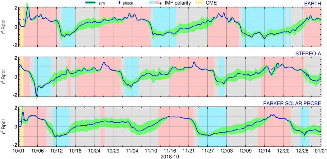
FIGURE 1. Predicted IMF polarity and crossings of the HCS at Earth, STEREO-A, and PSP (from top to bottom) from 2018-10-01 to 2018-12-31. The light-blue and light-red shading corresponds to negative (toward the Sun) and positive (away from the Sun) IMF polarity. A blue line shows the magnetic field polarity tracer (B_P). The light-green shading displays a range of B_P values at 4° above and below the spacecraft position, and the light-grey shading shows the corresponding inaccuracy in time.

Recently, Dresing et al. (2023) used ENLIL simulations at CCMC for a global context for their SEP study in mid-April 2021. They presented an evolution of the IMF components for BepiColombo, PSP, Solar Orbiter, STEREO-A, and near-Earth spacecraft. The simulated polarity agrees with the measurements at near-Earth and STEREO, but it is the opposite of the measurements by Solar Orbiter and BepiColombo. This remarkable difference is only for these two spacecraft locations; for other spacecraft, the B_ϕ component is more or less well simulated. We recomputed this scenario with the new ENLIL version to check this discrepancy. We used the WSA-5.4 maps (https://ccmc.gsfc.nasa.gov/models/WSA 5.4) and CME parameters in Table 1 for heliospheric simulation from 2021-04-17T00 to 2021-04-24T00 (7 days). In this period, the CCMC CME Scoreboard lists 2 observed shock arrivals at Earth, on 2021-04-15T03:28Z and 2021-04-22T08:50Z. The ICMECAT catalog lists 1 CME arrival at BepiColombo, on 2021-04-19T11:42Z but none at near-Earth, Solar Orbiter, or STEREO-A for that period.

TABLE 1

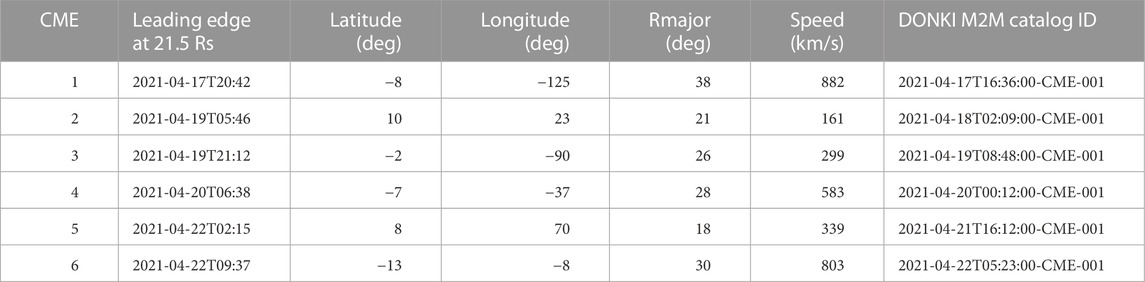
TABLE 1. Geometric and kinematic parameters of CMEs in mid-April 2021 (from DONKI catalog for ENLIL simulation with results shown in Figure 2).

Figure 2 shows a snapshot from our heliospheric simulation on 2021-04-19T00, together with the evolution of the predicted and measured values at the Solar Orbiter. Values at the ecliptic plane show that the Solar Orbiter is clearly in the positive sector, far away from the HCS, but values at the meridional slice show that the Solar orbiter is in the negative sector. The HCS has a very low inclination to the ecliptic, which complicates the reliable prediction of the HCS crossing. The light-green shading in Panel (c) indicates the range of predicted values at nearby latitudinal positions by 4° above and below the spacecraft position. These positions correspond to the dashed black lines in Panel (b). Results are for computation on a low-resolution grid [angular spacing of 4°, as used by Dresing et al. (2023)], but the same discrepancy is on a medium-resolution grid (2° angularly). We conclude that it is impossible to provide reliable predictions of the IMF polarity when the HCS is parallel to the spacecraft trajectory and within 1-2 computational cell(s) away from the spacecraft.

FIGURE 2

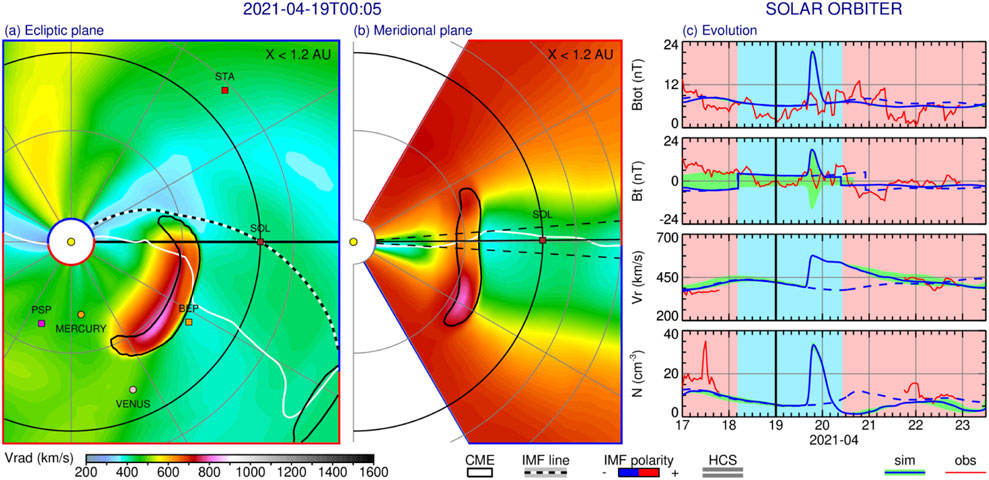
FIGURE 2. Simulated heliospheric disturbance on 2021-04-19T00. Panels (A,B) show the radial SW velocity (color scale) at ecliptic and meridional planes, respectively. A CME is outlined by a black contour, and the HCS is shown by a white line. The projected 3D IMF line passing through Solar Orbiter is shown by a black-white zebra line. Negative (positive) polarity is indicated by the blue (red) color at the region boundaries. Planetary and spacecraft positions are indicated by small spheres and boxes, respectively. Dashed lines in Panel (B) show latitudes by 4° above and below the spacecraft position. Panel (C) shows the evolution of the total magnetic field strength, tangential magnetic field, radial SW velocity, and number density (from top to bottom) at Solar Orbiter. Red lines show measured values. Solid (dashed) blue lines show the numerical solution with (without) CME-like disturbance. Negative (positive) polarity is indicated by the light-blue (light-red) shaded plot background. The light-green shading indicates the range of values at nearby latitudinal positions by 4° above and below the spacecraft position. The thick vertical black line marks the time of the snapshots in panels (A,B).

Note that the WSA model (1) assumes the coronal magnetic field is potential and (2) provides coronal maps at 21.5 Rs with an angular resolution of 2°, and these features limit the accuracy of heliospheric simulations. However, the main limitation is caused by the absence of magnetic field observations over the entire Sun. For example, on 2021-04-17, the Earth is by 5.5° below the equatorial plane; i.e., the photospheric magnetic field was observed at the Sun’s Southern Pole but not at the North Pole. Coronal models must use some assumptions to get complete input data (like using values from older observations) to calculate a complete coronal magnetic field. And this uncertainty in the strength of the polar magnetic field can easily lead to a few degrees of inaccuracy in the latitudinal current sheet position. Therefore, it is generally impossible to provide reliable predictions of the IMF polarity (and HCS crossings) if the HCS is flat and close to spacecraft positions. The presented visualization helps to identify such situations.

4 Tracing hydrodynamic ejecta

As given in Section 2, ENLIL can use additional continuity equations to trace the injected plasma material, and it can compute on multi-blocks to identify CME-driven transient disturbances. If these features are used together, we have a robust tool to analyze and predict transient heliospheric disturbances. This tool can be used to differentiate between the arrival time of the CME ejecta (using the D_P tracer) and surrounding CME-driven disturbance (using a multi-block approach). This increases confidence in the case of glancing-blow CMEs, and it may also help identify individual CMEs’ contribution in the case of multi-CME events.

Odstrcil et al. (2020) showed that tracking faint CMEs is challenging because there is no significant difference between the speeds of the CME and background SW the CME rides on, and weak dynamic interaction in the heliosphere leads only to a slight distortion of the background SW. This is even more of a problem if small-scale “blobs” are present in time-dependent simulations with recently available high-cadence (1 or 2 h) WSA-5* maps. Odstrcil et al. (2020) showed that the multi-block technique helps to identify transient disturbances in such situations better. The authors used two computational blocks with identical numerical grids and the same numerical timestep to separately simulate the background SW and the background SW with all active CMEs. This allowed them to subtract the highly irregular background SW solution and track contributions from the CME-driven disturbances while allowing the CMEs to interact during propagation.

As given in Section 2, the CME ejecta is tracked by solving another continuity equation for the D_P quantity, this quantity is scaled by 1/r², and the CME extension is approximately outlined by a contour at 20% of its initial values at the inner boundary (0.1 AU). The same initial value of the tracing quantity D_P is used for all CMEs. This enables us to use the same threshold value and visualize all CMEs in the heliospheric domain irrespective of the CME density enhancement and density of the background SW.

Table 2 lists 6 CMEs that were operationally fitted at CCMC and are used here for our heliospheric simulations from 2022-03-28T00 to 2022-04-06T00 (9 days). At CCMC’s CME Scoreboard (https://kauai.ccmc.gsfc.nasa.gov/CMEscoreboard), all these CMEs were predicted to arrive at Earth, but there were 2 observed shock arrivals at Earth in this period: 2022-03-31T01:41Z (merged CME 1 and CME 2) and 2022-04-06T22:45Z (CME 6). There were three false alarms (predicted shock arrival, but nothing was observed at Earth) for CMEs 3, 4, and 5. The ICMECAT catalog (https://helioforecast.space/icmecat) lists ICME arrival at the Wind spacecraft on 2022-03-31T01:40 (merged CME 1 and CME 2) but has no entry for CME.

TABLE 2

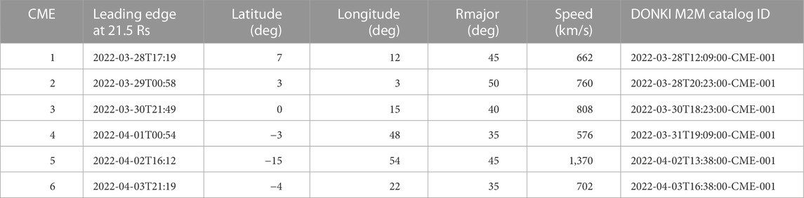
TABLE 2. Geometric and kinematic parameters of CMEs in late-March 2022 (from DONKI catalog for ENLIL simulation with results shown in Figures 3, 5).

Figure 3 shows an example of tracking individual CMEs listed in Table 2. We used 7 computational blocks to relate heliospheric disturbances to their coronal sources. The output of the computation on blocks is used to identify individual CMEs and also to visualize their approximate shape at the ecliptic plane. Left panel shows a snapshot of the SW density caused by CMEs 1, 2, and 3 on 2022-04-01T00. Faster CME 2 (light-green) overtook CME 1 (light blue), and the combined ejecta will pass through Earth and STEREO-A (also defunct STEREO-B). Note that the CMEs 1 + 2 are distorted during propagation through the structured solar wind. CME 3 (light-orange) is trailing behind and just about to sweep over BepiColombo and Venus.

FIGURE 3

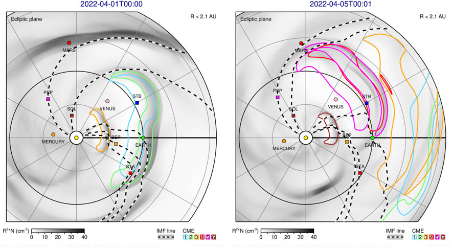
FIGURE 3. Heliospheric disturbances on 2022-04-01T00 (left panel) and 2022-04-05T00 (right panel). Normalized SW at the ecliptic is shown by grey shading with a color bar at the bottom left of each panel. Individual CMEs are outlined by contour lines with different colors, as given at the bottom right of each panel. The projected 3D IMF lines passing through BepiColombo (BEP), Earth, Parker Solar Probe (PSP), Solar Orbiter (SOL), and STEREO-A (STA) are shown by the black-white zebra lines. Planetary and spacecraft positions are indicated by small spheres and boxes, respectively.

Right panel shows a snapshot of the SW density for all 6 CMEs on 2022-04-05T00. Merged CMEs 1 and 2 are leaving the computational domain, and CME-3 closely follows them. There is another merge of CME 4 (red) and CME 5 (magenta), and this structure may be hitting Earth with a glancing blow (shock flank). CME 6 (brown) is far behind and about to reach BepiColombo.

Different parts of the CME-driven disturbances can hit Earth, and this can initiate different processes in the geospace. Namely, the flank hits (glancing blows) include shock (or compression pressure wave), while apex hits (full blows) can include both shock and magnetic ejecta. Our new tool helps to differentiate between the arrival of the CME ejecta (using the D_P tracer) and CME-driven disturbance in the surrounding SW (using a multi-block approach). This will help forecasters to differentiate between a direct hit and a glancing blow.

5 Detection of interplanetary shock arrivals

The most important question for space weather forecasting is: when will the CME-driven disturbances arrive? This is challenging to answer because 1) background SW is structured and evolving, 2) stream interactions may lead to the formation of a corotating shock-pair structure, 3) the need to identify the forward shocks only (reverse shocks are much weaker, but numerical simulations with transients launched in the super-critical outflow emphasize them, and 4) multiple CMEs that may mutually interact. Yet, automatic detection of shocks and their arrival times at different observers will help space weather forecasters.

We simulated heliospheric disturbances from 2022-08-14T00 to 2022-08-23T00 (9 days). There were 7 CMEs propagating in similar directions, which suggests their multiple interactions. Table 3 lists their parameters operationally fitted at CCMC. There were 3 observed shock arrivals at Earth: 2208-17T02:16Z (merged), 2022-08-19T17:02Z, and 2022-08-20T17:24Z, listed at CCMC CME Scoreboard). There is no CME arrival at Earth in the ICMECAT catalog. We computed this scenario with 7 CMEs on 8 computational blocks.

TABLE 3

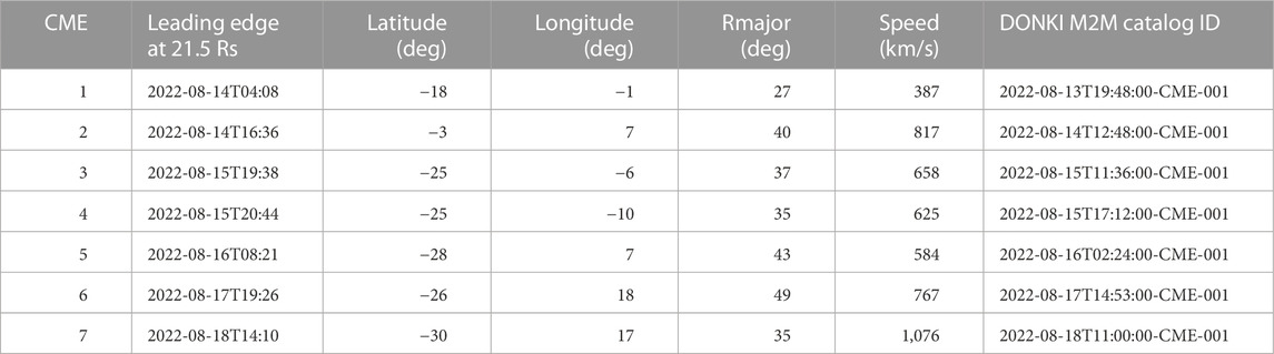
TABLE 3. Geometric and kinematic parameters of CMEs in mid-August 2022 (from DONKI catalog for ENLIL simulation with results shown in Figure 2).

Figure 4 shows the evolution of radial SW velocity at Earth as computed on 8 computational blocks. These blocks correspond to the number of CMEs plus one block for the background-only SW. The first block always has the complete solution (with all CMEs), and the last block always has the background-only solution (block 8 in our case). Figure 4 show results for:

(a) background and CME 1 (computed on block 7). It can be seen that the CME-1 (light-blue) has basically no effect at Earth.

(b) background and CMEs 1-2 (computed on block 6). The CME-2 (light-green) overtook the eventual effects of CME-1, and its shock (green) arrived at Earth close to observations.

(c) background and CMEs 1-3 (computed on block 5). CME 3 (light-orange) propagates on top of the preceding disturbance and drives a shock (08-18T11:01), but no shocks were observed around this time.

(d) background and CMEs 1-4 (computed on block 4). CME 4 (light-red) is a glancing blow with an ejecta seen around 08-19 without a shock but slightly modifying the previous shock propagation.

(e) background and CMEs 1-5 (computed on block 3). CME-5 (light-grey) propagates on top of the previous disturbances and drives a shock (dark grey, 08-19T01:42); no shock was observed around this time, but by 15:20 later

(f) background and CMEs 1-6 (computed on block 2). CME-6 (light blue) propagates on tails of previous disturbances and drives a shock (blue, 08-20T05:58); no shock was observed around this time, but by 11:04 earlier or 11:26 later

(g) background and CMEs 1-7 (computed on block 1). CME-7 (light-grey) propagates on top of CME-6 driven disturbance and drives a shock (green, 08-20T21:33), which is later than the observed shock by 4:19. This is a complete solution for the given period.

FIGURE 4

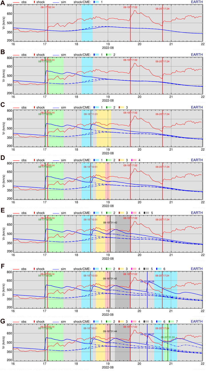
FIGURE 4. Evolution of the radial SW velocity at Earth from 2022-08-16 to 2022-08-22. The red and blue lines show the measured values and numerical simulations, respectively. Solid blue lines show the complete simulation, and dashed and dash-dot blue lines show the solution without the latest CME-like disturbance. Vertical red lines show observed shock arrivals. Simulated shock arrivals and driving CMEs are shown by colored vertical lines and shaded areas for individual CMEs as labeled on the top of each plot. (A–G) show computations with different number of CMEs and blocks as given in the text.

Such a visualization enables us to identify the contribution of individual CMEs and adjust their parameters if necessary for better reconstruction of historical events.

6 Shock parameters and alerts

ENLIL can calculate the topology of IMF lines passing through observers (planets, spacecraft, or user-specified positions), extract SW parameters along those lines, check whether this vantage point is magnetically connected to a CME-driven shock, and if yes, then determine its MHD shock parameters. As a result, the available ENLIL output includes files with time sequences of the observer’s IMF lines saved at a 5-min cadence, together with files describing any shocks along those IMF lines (one file for each observer for each CME). Note that (1) such high cadence is achieved by linear interpolation from 3D output files produced with a 1-h cadence, and (2) the inner boundary of ENLIL at 21.5 Rs limits the ability to include the coronal portions of the fields and shocks.

The SEPMOD code (Luhmann et al., 2007) can use those files and produce SEP flux-time series at all observers magnetically connected to ENLIL shocks. These time series represent the SEPs produced by shocks beyond the ENLIL 21.5 Rs boundary unless a separate flare or coronal influx is imposed there as a boundary source option. Luhmann et al. (2007) used a heliospheric MHD simulation for a single CME event and found that the combination of a relatively simple description based on the diffusive shock acceleration process at the shock location, followed by scatter-free propagation along the ENLIL field lines can approximate an observed SEP time profile. Luhmann et al. (2017) later demonstrated a SEPMOD version that accommodates multiple concurrent shock sources. ENLIL uses two computational blocks to identify shocks and determine their MHD parameters. One block is for computing all CMEs, and the second block is for computing only background conditions. ENLIL produces a file of the related shock parameters for each CME in the run. SEPMOD is then run for each CME, using its specific shock parameters, but with the observer-connected field lines from the comprehensive (all CMEs included) ENLIL runs for transport. The addition of the SEPMOD SEP flux profiles from the individual ENLIL CME shock sources then produces the overall SEP flux time series for the period of the ENLIL run. Recently, we extended the multi-block approach to possibly use more than 2 blocks to produce the files for SEPMOD. This reduces the inaccuracy when determining shock parameters along the IMF line, even in mutually interacting CMEs. SEPMOD calculates SEP fluxes independently for each CME-driven shock and sums them to provide the resulting SEP flux for each IMF line connected to the observer.

We have also developed global “alert” plots for providing prompt shock-associated SEP warnings. These plots indicate which sectors in the heliosphere might be affected by SEP fluxes if they propagate along the IMF lines from CME-driven shocks. These regions are colored, from yellow to red, according to the strength of the strongest shock magnetically connected to the observer. If the IMF line reaches the inner boundary of the computational domain without encountering any shock, this is considered an “all-clear” condition, and the sector is colored by a green shading corresponding to the radial SW velocity.

Figure 5 shows a snapshot of the shock-alert plot relevant to heliospheric disturbances on 2022-04-01T00. These disturbances are caused by the multi-CME events with initial parameters given in Table 2. Note that results from this simulation are also shown in Figure 3 at the same region and time. Left panel (a) shows results in the same region at the same time as in Figure 3 as in shock-alert plots. Firstly, a colored fan region is displayed as follows. From each grid point at the outer boundary of the computational domain, IMF lines are traced until an intersection with the strongest CME-driven shock is detected, and the sector is colored (from yellow to red) by the difference between the radial speeds of the disturbed and background states. If the IMF line reaches the inner boundary (at 0.1 AU) of the computational domain without encountering any shock, then the sector is colored by green shading corresponding to the radial SW velocity. Then, the density compression ratio (positive values only) are displayed using a grey scale to identify shock-compressed sheath regions, and the associated individual CMEs are outlined in different colors. Finally, the IMF lines passing through observers are shown by black-white zebra lines. Right panels (b-e) indicate the distance along the IMF lines between four spacecraft and the CME-driven shocks:

(b) Earth is magnetically connected to all shocks, both before (negative value) and after (positive value) their arrival at Earth driven by CME-1+2 on 03-28T19, CME-3 on 03-31T02, CME-4 on 04-01T02, CME-5 04-02T17, and CME = 6 on 04-04T00.

(c) Parker Solar Probe is longitudinally located westward from the propagating CMEs, but because of the spiraling IMF, the spacecraft is magnetically connected to shock flanks (after passing 1.5 AU) driven by CME-1+2 on 04-03T12, CME-3 on 04-04T23, and CME-4 on 04-05T01.

(d) Solar Orbiter is connected to shocks at larger distances (as is the case with Parker Solar Probe, but to a greater number of shocks because of close longitudinal separation) driven by CME-1+2 on 03-31T06, CME-3 on 04-03T05, and CME-4 on 04-03T08.

(e) STEREO-A is located eastward of centers of propagating CMEs, and thus, it is connected to their shocks before their arrivals (this connection is lost later) driven by CME-1+2 on 03-28T18, CME-3 on 03-30T23, CME-4 on 04-01T04, CME-5 on 04-02T17, and CME-6 on 04-03T23.

FIGURE 5

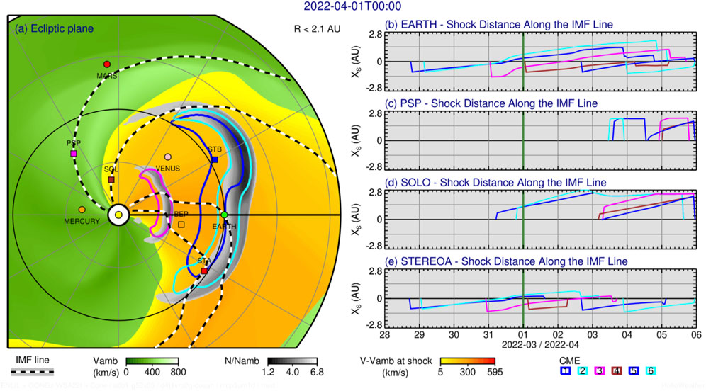
FIGURE 5. Shock alert plots for multi-CME events on 2022-04-01T00. Left panel (A) shows the background SW velocity (green scale), density compression ratio at the leading edge of transients (dark-grey scale), the extent of the driving CMEs (contours with colors for individual CMEs given at the bottom right), sectors colored by the shock strength (from yellow to red). The projected 3D IMF lines passing through Earth, PSP, Solar Orbiter, and STEREO-A are shown by black-white zebra lines. Planetary and spacecraft positions are indicated by small spheres and boxes, respectively. Right panel (B–E) shows the distance along the IMF line between the spacecraft and the shock front. Negative (positive) values indicate that the shock front is approaching (leaving) the spacecraft.

Note that these IMF lines and shock identifications can also be found in the files produced for the SEPMOD. This tool can help space weather forecasters and researchers by providing a global context and guidance for identifying individual shock-observer connections and issuing SEP alerts.

7 Synthetic WL imaging

Simulated 3D distributions of the SW density can be used to calculate synthetic images of the WL brightness as they are remotely observed by heliospheric imagers (HI). We integrate the Thomson scattering formulae (Hundhausen, 1993) along the line-of-sight (LOS) from a given observer’s location through the heliosphere (Odstrcil et al., 2005; Odstrcil and Pizzo, 2009). ENLIL produces synthetic images of the total and polarized WL brightness within the angular sector +/-60° away from the equatorial plane and for elongation angles from 6° to 90° from the Sun-observer line. We developed this capability for the HIs onboard the twin STEREO spacecraft (Odstrcil et al., 2005), but we have generalized its functionality for imagers of the recently-launched PSP and Solar Orbiter (Odstrcil et al., 2020) and upcoming PUNCH (Polarimeter to Unify the Corona and Heliosphere) spacecraft.

The synthetic WL images can assist in the interpretation of remote heliospheric observations of WL scattered on the density structures (Odstrcil et al., 2005; Odstrcil and Pizzo, 2009; Howard et al., 2013), and they can also be used for “mid-course” correction of heliospheric space weather predictions. The appearance of WL structures depends strongly on their location with respect to the so-called Thomson surface, where the scattering response is greatest Vourlidas and Howard (2006). Thus, the interpretation of HI observations is not straightforward. This is especially true if CMEs: 1) are slow and weak events that slightly disturb the background SW; 2) propagate farther away from the Thomson surface; 3) propagate in highly structured SW with varying densities. In addition, using newer versions of WSA coronal maps (https://ccmc.gsfc.nasa.gov/models/WSA 5.4) introduce density fluctuations in the ambient SW that can hamper the identification and tracking of CMEs. These density structures also experience Thomson scattering and may have a similar magnitude as the WL intensities of comparable CMEs. Therefore, we have developed a novel “ambient-difference” approach (Odstrcil et al., 2020) to track weak CMEs in which we use a multi-block technique to: 1) compute density distributions with and without transient disturbances; 2) calculate synthetic WL images for both scenarios; and 3) display the WL images as a difference between disturbed and ambient states (“adif”). This enhances the current visualization possibilities of absolute values (“abs”), the running difference (“rdif”), the running ratio (“rrat”), and elongation-scaled values (“elon”). Note that the “adif” approach adds inaccuracy between the simulated and actual SW density into the visualization. However, this approach is very helpful because it removes the effect of artificially introduced density fluctuations.

Figure 6 shows a snapshot from simulated hypothetical heliospheric disturbances for December 2025, during the planned one-month-long Artemis III mission to the Moon (https://www.nasa.gov/feature/artemis-iii). We used the 11-year solar activity cycle to project heliospheric space weather into the future. Planetary and spacecraft positions are displayed as of December 2025, but the background SW and CMEs data are from December 2014. Table 4 lists 36 CMEs operationally fitted at CCMC, and this busy scenario is used to verify the new modeling system. We conduct a simulation experiment to see how the PUNCH spacecraft (planned launch in April 2025) can be used to improve operational predictions of heliospheric space weather. Figure 6 shows that STEREO-A will be in a very good position for mid-course evaluation of ENLIL ensemble simulations and can be used to prune ensemble members with observations for a more accurate prediction. It is possible to use the Cartesian projection for the elongation-phase plots to see better eventual distortions of the CME-driven disturbances.

FIGURE 6

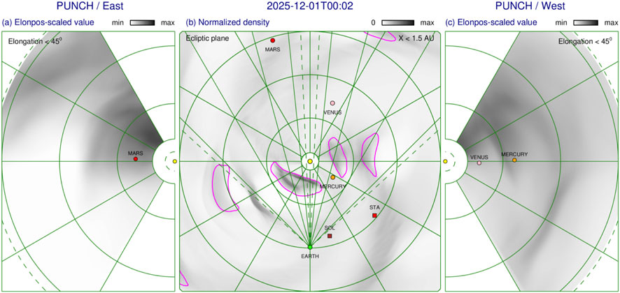
FIGURE 6. Simulated heliospheric disturbances as might be observed from the PUNCH spacecraft in December 2025. Planetary and spacecraft positions are displayed as of December 2025, but background SW and CMEs data are from December 2014. Panel (B) shows the normalized SW density at the equatorial plane using a grey scale given at the top. Planetary and spacecraft positions are indicated by small spheres and boxes, respectively. The PUNCH combined field of view (1.5°–48°) is shown by dashed green lines. Solid green lines correspond to the elongations of the inner boundary and to 15°, 30°, and 45°. Green concentric rings show heliospheric distances at 0.1, 0.5, 1, and 1 AU. Panel (A,C) Panel show the total WL brightness eastward and westward from the Sun, respectively.

TABLE 4

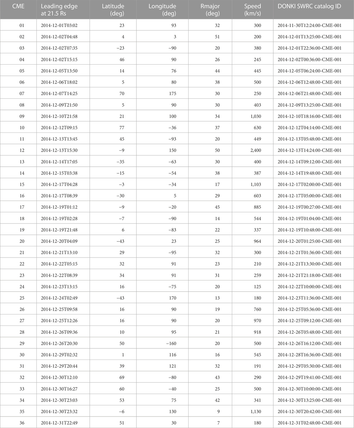
TABLE 4. Geometric and kinematic parameters of CMEs in December 2014 (from DONKI catalog for ENLIL simulation with results shown in Figure 6).

8 Conclusion

The WSA-ENLIL-Cone modeling system can routinely simulate continuously evolving background SW and all observed CMEs, event-by-event, and much faster than real-time. This modeling system has been used for various research applications and operational space weather predictions. In this paper, we described features not routinely used at space weather prediction centers and/or provided by NASA/CCMC Run-On-Request service, and we showed their benefits when applied to multi-CME events observed by various spacecraft. We used the WSA coronal maps and CME parameters from the DONKI catalog and simulated selected heliospheric space weather events relevant to the current PSP, Solar Orbiter, and STEREO-A missions, and to the planned PUNCH mission. We presented new ENLIL features and visualization concepts that provide a more informative description of the heliospheric space weather situation and can assist in (1) the interpretation of remote observations and in-situ measurement of multi-CME events at various spacecraft and (2) operational prediction of the arrival time of CMEs at Earth and other objects.

ENLIL heliospheric simulations can predict the HCS topology as a thin structure without magnetic reconnection. This is achieved by computing the IMF as monopolar and solving an additional equation for tracking the polarity. However, it is challenging to predict the HCS crossing when the spacecraft trajectory is close to the flat HCS. We developed a tool that helps to evaluate the accuracy of such predictions and will mark periods with less reliable predictions. We record values of the polarity tracing quantity at the latitudes above and below spacecraft positions, determine the corresponding temporal range, and display these values on ENLIL-produced plots.

Tracking CMEs accurately is another challenging task, especially if (1) CMEs are weak (and they cause only small density compression in the interplanetary medium) or (2) there are multiple CMEs active at the same time (and their interaction makes it difficult to separate their impact). We used an additional continuity equation to trace the injected CME material and multi-block computations to identify transient disturbances. This allowed us to subtract the background SW solution and track contributions from CME-driven disturbances while still allowing the CMEs to interact during propagation. This approach enables reliable tracking of CME propagation in the heliosphere, especially if CMEs are weak and their densities are comparable to small-scale density blobs or if CMEs propagate in complex SW stream structures. And this method enables robust automatic detection of shock arrivals at planets and spacecraft.

The multi-block computations also allow us to connect individual CME-driven shocks and the observers with the IMF line. This is helpful in (1) providing a global context for research studies of long-duration SEP events; (2) identification of all shock parameters along the IMF lines for SEP models like SEPMOD; and (3) production of shock alert plots in the case of multiple-CMEs.

We also extended our multi-block approach to assist in interpreting the WL structures observed by heliospheric imagers. The subtraction of disturbed and undisturbed WL images shows a clear signal of the CME against the background SW structures. This approach is especially helpful if CMEs: (1) are slow and weak events that slightly disturb the background SW; (2) propagate farther away from the Thomson surface; and (3) propagate in highly structured SW with varying densities. Comparison with observed WL structures can be used for mid-course correction of the CME arrival times or for pruning ensemble members, which would have an unrealistic projected arrival time.

The WSA-ENLIL-Cone modeling system has been used for operational predictions of heliospheric space weather for 14 years. It can predict, on average, the arrival of CME-driven disturbances with an inaccuracy of 6–8 h (Mays et al., 2020). However, no significant improvement was reached over the last 10 years (Riley et al., 2018). Moreover, the arrival time error can occasionally be large ($>$ 24 h, especially for hard-to-fit CMEs. This is caused by a lack of observational data to initialize numerical models in the solar corona, which prevents them from launching realistic CME-like transient disturbances. Another source of uncertainties is the background SW itself, where the CME disturbances ride on. Photospheric magnetic field observations used by the WSA model cover only a small fraction of the domain, and there is a lack of far-side information. All this prevents realistic simulations of the background SW and CMEs.

But the improvements in the operational predictions of heliospheric space weather can be achieved by ensemble simulations and by incorporating remote observations from heliospheric imagers. The former can account for uncertainties in the model initialization, and the latter can be used to weed out bad ensemble members, which would otherwise lead to unrealistic arrival time predictions. The position of the STEREO-A spacecraft will be favorable to support the upcoming Artemis missions, and we can use our “mid-course correction” method. A coordinated, collaborative effort is needed to better understand heliospheric space weather, validate numerical codes, and improve predictive ability.

Data availability statement

The raw data supporting the conclusion of this article will be made available by the authors, without undue reservation.

Author contributions

The author confirms being the sole contributor of this work and has approved it for publication.

Funding

This work has been partly supported by the NASA Space Weather Science Application Research-to-Operations-to-Research (R2O2R), Grant 80NSSC23K0451.

Acknowledgments

The background SW was computed from coronal maps produced by the WSA model that uses synoptic magnetograms from the Global Oscillation Network Group (GONG). Geometric and kinematic CME parameters were obtained from the NASA/CCMC Space Weather Database Of Notifications, Knowledge, Information (DONKI; https://kauai.ccmc.gsfc.nasa.gov/DONKI/). These parameters were fitted using the coronagraph observations at SOHO and STEREO-A spacecraft. Planetary and spacecraft positions are from NASA/GSFC Helioweb (https://omniweb.gsfc.nasa.gov/coho/helios/heli.html) and NASA/JPL Horizons (https://ssd.jpl.nasa.gov/horizons/) websites. In-situ measurements at ACE/Wind, BepiColombo, Parker Solar Probe, Solar Orbiter, and STEREO-A were obtained from the NASA/GSFC COHOweb (https://omniweb.gsfc.nasa.gov/coho/) website. Observed arrivals of interplanetary shocks are from NASA/CCMC CME-Scoreboard (https://ccmc.gsfc.nasa.gov/scoreboards/cme/) and EU/HELCATS ICMECAT (https://www.helcats-fp7.eu/catalogues/wp4_icmecat.html) catalog. In situ measurements at L1 and STEREO-A in situ were obtained from the NASA/GSFC COHOweb website. The author thanks Dr. Siegfried Gonzi (UK Met Office) for reviewing the manuscript and for helpful suggestions to improve the quality of the manuscript, and to Drs. Janet Luhmann (UC Berkeley), Vic Pizzo (NOAA/SWPC), Jie Zhang (George Mason University), and Leila Mays (NASA/CCMC) for helpful suggestions in improving the quality of the manuscript. We appreciate the careful review by two referees that helped improve the paper’s quality.

Conflict of interest

The author declares that the research was conducted in the absence of any commercial or financial relationships that could be construed as a potential conflict of interest.

Publisher’s note

All claims expressed in this article are solely those of the authors and do not necessarily represent those of their affiliated organizations, or those of the publisher, the editors and the reviewers. Any product that may be evaluated in this article, or claim that may be made by its manufacturer, is not guaranteed or endorsed by the publisher.

References

Arge, C. N., and Pizzo, V. J. (2000). Improvement in the prediction of solar wind conditions using near-real-time solar magnetic field updates. J. Geophys. Res. 105, 10465–10479. doi:10.1029/1999JA000262

CrossRef Full Text | Google Scholar

Dresing, N., Rodriguez-Garcia, L., Jebaraj, I. C., Warmuth, A., Wallace, S., Balmaceda, L., et al. (2023). The 17 April 2021 widespread solar energetic particle event. Available at: https://arxiv.org/abs/2303.10969 (Accessed March 20, 2023).

Google Scholar

Howard, T. A., Tappin, S. J., Odstrcil, D., and DeForest, C. E. (2013). The Thomson surface. III. Tracking features in 3D. Astrophys. J. 765, 45. doi:10.1088/0004-637X/765/1/45

CrossRef Full Text | Google Scholar

Hundhausen, A. J. (1993). Sizes and locations of coronal mass ejections: SMM observations from 1980 and 1984-1989. J. Geophys. Res. 98, 13177–13200. doi:10.1029/93JA00157

CrossRef Full Text | Google Scholar

Luhmann, J. G., Ledvina, S. A., Krauss-Varban, D., Odstrcil, D., and Riley, P. (2007). A heliospheric simulation-based approach to SEP source and transport modeling. Adv. Space Res. 40 (3), 295–303. doi:10.1016/j.asr.2007.03.089

CrossRef Full Text | Google Scholar

Luhmann, J. G., Mays, M. L., Odstrcil, D., Li, Y., Bain, H., Lee, C. O., et al. (2017). Modeling solar energetic particle events using ENLIL heliosphere simulations. Space weather. 15, 934–954. doi:10.1002/2017SW001617

CrossRef Full Text | Google Scholar

Mays, M. L., MacNeice, P., Taktakishvili, A., Wiegand, C. P., Merka, J., Adamson, E. T., et al. (2020). NASA/NOAA MOU Annex Final Report: Evaluating model advancements for predicting CME arrival time. Available at: https://ccmc.gsfc.nasa.gov/static/files/CCMC_SWPC_annex_final_report.pdf.

Google Scholar

Millward, G., Biesecker, D., Pizzo, V., and de Koning, C. A. (2013). An operational software tool for the analysis of coronagraph images: Determining CME parameters for input into the WSA-ENLIL heliospheric model. Space weather. 11 (2), 57–68. doi:10.1002/swe.20024

CrossRef Full Text | Google Scholar

Odstrcil, D., Dryer, M., and Smith, Z. (1996). Propagation of an interplanetary shock along the heliospheric plasma sheet. J. Geophys. Res. 101, 19973–19986. doi:10.1029/96JA00479

CrossRef Full Text | Google Scholar

Odstrcil, D., Mays, M. L., Hess, P., Jones, S. I., Henney, C. J., and Arge, C. N. (2020). Operational modeling of heliospheric space weather for the Parker Solar Probe. Astrophys. J. Suppl. Ser. 246 (2), 73. doi:10.3847/1538-4365/ab77cb

CrossRef Full Text | Google Scholar

Odstrcil, D. (2003). Modeling 3-D solar wind structure. Adv. Space Res. 32 (4), 497–506. doi:10.1016/s0273-1177(03)00332-6

CrossRef Full Text | Google Scholar

Odstrcil, D., Pizzo, V. J., and Arge, C. N. (2005). Propagation of the 12 May 1997 interplanetary coronal mass ejection in evolving solar wind structures. J. Geophys. Res. 110, A02106. doi:10.1029/2004JA010745

CrossRef Full Text | Google Scholar

Odstrcil, D., and Pizzo, V. J. (1999b). Distortion of the interplanetary magnetic field by three-dimensional propagation of coronal mass ejections in a structured solar wind. J. Geophys. Res. 104, 28225–28239. doi:10.1029/1999JA900319

CrossRef Full Text | Google Scholar

Odstrcil, D., Pizzo, V. J., Linker, J. A., Riley, P., Lionello, R., and Mikic, Z. (2004b). Initial coupling of coronal and heliospheric numerical magnetohydrodynamic codes. J. Atmos. Solar-Terr. Phys. 66, 1311–1320. doi:10.1016/j.jastp.2004.04.007

CrossRef Full Text | Google Scholar

Odstrcil, D., and Pizzo, V. J. (2009). Numerical heliospheric simulations as assisting tool for interpretation of observations by STEREO heliospheric imagers. Sol. Phys. 259, 297–309. doi:10.1007/s11207-009-9449-z

CrossRef Full Text | Google Scholar

Odstrcil, D., and Pizzo, V. J. (1999a). Three-dimensional propagation of coronal mass ejections (CMEs) in a structured solar wind flow: 1. CME launched within the streamer belt. J. Geophys. Res. 104, 483–492. doi:10.1029/1998JA900019

CrossRef Full Text | Google Scholar

Odstrcil, D., Riley, P., and Zhao, X. P. (2004a). Numerical simulation of the 12 May 1997 interplanetary CME event. J. Geophys. Res. 109, A02116. doi:10.1029/2003JA010135

CrossRef Full Text | Google Scholar

Pizzo, V. (1982). A three-dimensional model of corotating streams in the solar wind: 3. Magnetohydrodynamic streams. J. Geophys. Res. 87, 4374. doi:10.1029/JA087iA06p04374

CrossRef Full Text | Google Scholar

Pizzo, V., Millward, G., Parsons, A., Biesecker, D., Hill, S., and Odstrcil, D. (2011). Wang-Sheeley-Arge-Enlil Cone model transitions to operations. Space weather. 9, S03004. doi:10.1029/2011SW000663

CrossRef Full Text | Google Scholar

Poedts, S., Lani, A., Scolini, C., Verbeke, C., Wijsen, N., Lapenta, G., et al. (2020). European heliospheric FORecasting information asset 2.0. J. Space Weather Space Clim. 10, 57. doi:10.1051/swsc/2020055

CrossRef Full Text | Google Scholar

Pomoell, J., and Poedts, S. (2018). Euhforia: European heliospheric forecasting information asset. J. Space Weather Space Clim. 8, A35. doi:10.1051/swsc/2018020

CrossRef Full Text | Google Scholar

Riley, P., Mays, M. L., Andries, J., Amerstorfer, T., Biesecker, D., Delouille, V., et al. (2018). Forecasting the arrival time of coronal mass ejections: Analysis of the CCMC CME Scoreboard. Space weather. 16, 1245–1260. doi:10.1029/2018SW001962

CrossRef Full Text | Google Scholar

Taktakishvili, A., MacNeice, P., and Odstrcil, D. (2010). Model uncertainties in predictions of arrival of coronal mass ejections at Earth orbit. Space weather. 8, S06007. doi:10.1029/2009SW000543

CrossRef Full Text | Google Scholar

Totten, T. L., Freeman, J. W., and Arya, S. (1995). An empirical determination of the polytropic index for the free-streaming solar wind using Helios 1 data. J. Geophys. Res. 100 (A1), 13–18. doi:10.1029/94JA02420

CrossRef Full Text | Google Scholar

Totten, T. L., Freeman, J. W., and Arya, S. (1996). Application of the empirically derived polytropic index for the solar wind to models of solar wind propagation. J. Geophys. Res. 101 (A7), 15629–15635. doi:10.1029/96JA01019

CrossRef Full Text | Google Scholar

Vourlidas, A., and Howard, R. A. (2006). The proper treatment of coronal mass ejection brightness: A new methodology and implications for observations. Astrophys. J. 642, 1216–1221. doi:10.1086/501122

CrossRef Full Text | Google Scholar

Vourlidas, A., Patsourakos, S., and Savani, N. P. (2019). Predicting the geoeffective properties of coronal mass ejections: Current status, open issues and path forward. Philosophical Trans. R. Soc. Lond. Ser. A 377 (2148), 20180096. doi:10.1098/rsta.2018.0096

CrossRef Full Text | Google Scholar

Winterhalter, D., Smith, E. J., Burton, M. E., Murphy, N., and McComas, D. J. (1994). The heliospheric plasma sheet. J. Geophys. Res. 99, 6667–6680. doi:10.1029/93JA03481

CrossRef Full Text | Google Scholar

Wold, A. M., Mays, M. L., Taktakishvili, A., Jian, L. K., Odstrcil, D., and MacNeice, P. (2018), Verification of real-time WSA-ENLIL+Cone simulations of CME arrival-time at the CCMC from 2010 to 2016, J. Space Weather Space Clim. 8, A17, 12 pp, doi:10.1051/swsc/2018005

CrossRef Full Text | Google Scholar

Xie, H., Ofman, L., and Lawrence, G. (2004). Cone model for halo CMEs: Application to space weather forecasting. J. Geophys. Res. 109, A03109. doi:10.1029/2003JA010226

CrossRef Full Text | Google Scholar

Zhao, X., and Dryer, M. (2014). Current status of CME/shock arrival time prediction. Space weather. 12, 448–469. doi:10.1002/2014SW001060

CrossRef Full Text | Google Scholar

Zhao, X. P., Plunkett, S. P., and Liu, W. (2002). Determination of geometrical and kinematical properties of halo coronal mass ejections using the cone model. J. Geophys. Res. 107, SSH 13-21–SSH 13-19. doi:10.1029/2001JA009143

CrossRef Full Text | Google Scholar