Exploring intermittency in numerical simulations of turbulence using single and multi-spacecraft analysis

1 Introduction

The solar wind, a fundamental component of our Solar System, plays a crucial role in shaping the dynamic interactions between the Sun and the surrounding space environment. This continuous stream of charged particles, primarily electrons and protons, emanates from the Sun’s outermost layer, the solar corona (Gosling, 2014). Over the decades, scientific inquiry has unravelled the intricate nature of the solar wind, revealing its multifaceted impact on celestial bodies, interplanetary space, and our understanding of astrophysical phenomena. At its origin, the solar wind consists of high-energy particles with velocities exceeding 400 km per second Marsch et al. (1982). These particles escape the Sun’s gravitational pull and radiate outward in all directions, filling the entire Solar System, and becoming a prominent ingredient for the space weather. These charged particles carry with them the Sun’s magnetic field, forming a complex and dynamic structure known as the interplanetary magnetic field (IMF).

The fluctuations of the magnetic field associated with charged particles are a dynamic and intriguing phenomenon and are an integral part of the interplay between the Sun and the surrounding interplanetary medium. The accurate statistical description of the magnetic field fluctuations is important because it provides valuable insights into the underlying physical processes that govern these variations. By quantifying the statistical properties of magnetic field fluctuations, such as their amplitude, frequency, and spatial distribution, the patterns, correlations, and anomalies within the data can be discerned (Goldstein et al., 1994).

Intermittency in the solar wind refers to the phenomenon where energy at a given scale is not uniformly distributed in space (Bruno, 2019). This intermittency is linked to the non-Gaussian nature of turbulent fluctuations, with non-Gaussianity increasing at smaller scales. Instead of a uniform energy distribution, the solar wind tends to localise it in coherent structures, i.e., formations characterised by phase synchronisation across multiple scales (Perrone et al., 2017). Studying these current structures, which often give rise to what we term “coherent structures”, is directly related to energy dissipation processes typically manifesting in the so-called “energy cascades” (Dong et al., 2020). Analysing the statistics of the Probability Density Functions (PDFs) of increments provides valuable information about the distribution of coherent and intermittent structures. Notably, this method has been extensively investigated both using in-situ data and numerical simulations (Greco et al., 2009; Wu et al., 2013; Chhiber et al., 2018; Palacios et al., 2022).

It is anticipated that upcoming multi-point measurement missions, such as the Helioswarm mission (Klein et al., 2023), and mission concepts like MagneToRE (Maruca et al., 2021), will play a pivotal role in characterising current structures across various scales. Multi-spacecraft observations reveal a profound connection between space and time, as the same physical observables are measured not only at different spatial locations but also at different time instances. One of the primary challenges of multi-point measurement missions lies in reconstructing magnetic fields from data collected by distributed observatories. These innovative missions allow for diverse data analyses that enhance our understanding of turbulence and intermittency in the Earth’s magnetosphere as well as in the solar wind.

Although a robust study of the intermittency involves the characterisation of the high order moments of the PDF of the increments, the Partial Variance of Increments (PVI) method (Greco et al., 2008) is a simple tool to study coherent structures using in-situ data and numerical simulations. This method involves studying magnetic field increments at different scales along a single spacecraft trajectory. The PVI method has been extended to apply to measurements taken by missions with multiple spacecraft (Chasapis et al., 2015; Yordanova et al., 2016; Pecora et al., 2023), where measurements of the magnetic field by different nodes at the same time are compared. Recent studies have analysed in-situ data from a long-duration turbulent reconnection flow in Earth’s magnetotail (Chasapis et al., 2018; Huang et al., 2021). These studies are based on the analysis of statistics of magnetic field variation measured by various nodes of the MMS mission (PVI_m), and these distribution functions often follow Kappa distributions (Livadiotis and McComas, 2013).

In the present work, we study the probability distribution function (PDF) of magnetic field increments in a kinetic simulation of anisotropic plasma turbulence. We consider a single-spacecraft and a multi-spacecraft approach. We study the dependence of the PDF of the magnetic field increments on the angle between the scanning trajectory and the background magnetic field, which aligns with the z-axis. We also explore the dependence of the PDF of the PVI as a function of the scanning angle for both the single-spacecraft case and the multi-spacecraft case. In section 2 we describe the simulation and methods that we use. In section 3 we present our results. In section 4 we discuss their implications, and finally, we conclude and suggest future work paths.

2 Methodology

In this work, we use a particle-in-cell (PIC) simulation of anisotropic Alfvénic turbulence in an ion-electron plasma in the presence of a constant background magnetic field ${\mathbf{B}}_0=B_0\widehat{\mathbf{z}}$ to test our methods. The simulation domain is an elongated box of size L_x × L_y × L_z = 24d_i × 24d_i × 125d_i with spatial resolution Δx = Δy = Δz = 0.06d_i, where d_i = c/ω_pi is the ion inertial length, c is the speed of light, ${\omega }_{pi}=\sqrt{n_0{q}_i^2/m_i{ϵ}_0}$ is the ion plasma frequency and n₀ is the constant initial ion density. For details on the simulation see (Agudelo Rueda et al., 2021).

2.1 Synthetic data

We trace synthetic trajectories across the simulation domain to collect magnetic field measurements [see Figure 1A)]. In our approach, we use the Taylor hypothesis (Taylor, 1938) to treat the spatial and temporal variations interchangeably. Thus, we consider a data acquisition time f = 15 Hz and we assume the synthetic spacecraft sweeps the plasma with an average velocity v_sp = 400 km/s. Therefore, the resolution of our measurements and minimum lag is Δs = 0.3 d_i.

FIGURE 1

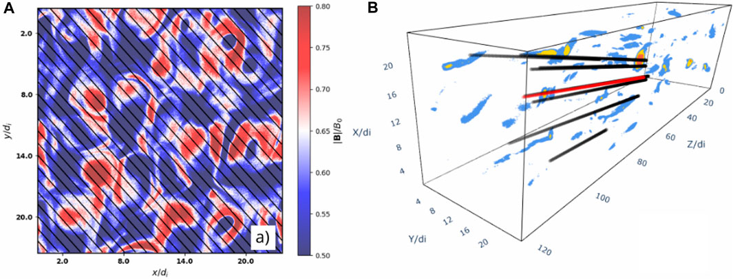
FIGURE 1. (A) Cross-section view of the simulation displaying the magnitude of the magnetic field. The diagonal lines represent the trajectories of a single spacecraft. (B) 3D view of the simulation domain. The colours represent different magnetic field thresholds. Regions with a more intense magnetic field are shown in red. The oblique lines are the virtual mission trajectories. The red line represents the hub, and the black lines represent the 8 nodes.

In the context of pioneering multi-point missions, HelioSwarm focuses on understanding solar wind dynamics at various scales (Plice et al., 2019). This mission involves the flight of a swarm of nine satellites (1 hub and 8 nodes) to measure multiple scales simultaneously. The distance between nodes will be focused in exploring the transition region from ion kinetic scales ∼ 100 km to MHD scale ∼ 1,200 km. Although the largest size of the simulation domain is $\sim 125d_i$, our results cover the small-scale range of scales be explored by Helioswarm $(\sim 1-100d_i)$.

The regions of interest for Helioswarm include the pristine solar wind, the Earth’s magnetosphere, and the magnetically connected region. In our study, we chose a spatial spacecraft configuration that corresponds to the configuration that the Helioswarm mission will display when traversing the pristine solar wind [see Figure 1B)]. The positions of the nodes with respect to the hub are shown in Table 1.

TABLE 1

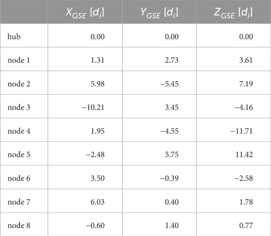
TABLE 1. The data represents the relative position of the HelioSwarm mission nodes in relation to the hub, expressed in units of d_i. The spacecraft configuration corresponds to the HelioSwarm when the mission passes through the solar wind. Retrieved from: https://eos.unh.edu/helioswarm/multimedia.

2.2 Partial variance of increments for single-spacecraft

We study the variation of the magnetic field vector calculated along a one-dimensional path, represented as ΔB = B(r + Δs) − B(r), where r is the position of the spacecraft and Δs represents a spatial lag in the collected data and we define the PVI index (Greco et al., 2018) as,

$PVI=\frac{|\mathrm{\Delta }\mathbf{B}\left(r,\mathrm{\Delta }s\right)|}{\sqrt{⟨|\mathrm{\Delta }\mathbf{B}\left(r,\mathrm{\Delta }s\right){|}^2⟩}},(1)$

here $⟨\dots ⟩$ represents the average over a sufficiently large interval. In our context, we apply this averaging process to all the data points within a trajectory. First, we investigate the behaviour of ΔB in a two-dimensional section of the simulation perpendicular to the background magnetic field $B_0\widehat{z}$. To do this, we take a cross-section slice in the xy-plane at z/di = 63.9 and we consider multiple trajectories on this plane resembling multiple crossings of a single spacecraft through the plasma, shown in Figure 1A). We also study the distribution of magnetic field increments when considering 3D trajectories across the entire simulation domain.

2.3 Partial variance of increments multi-spacecraft

We analyse the PDFs of ΔB for the data collected by the multi-spacecraft configuration. This is done using the aforementioned frequency and flow velocity. The analysis of the multi-point data is being carried out by comparing measurements taken by each pair of nodes at the same time. We examined the multi-point magnetic field variance, denoted as ΔB_ij(r) = Bⁱ(r) − B^j(r), where i and j represent individual nodes or hub, ranging from i, j = 1, 2, 3, … , 9, with i ≠ j. Thus, we define the PVI multi-spacecraft index as:

$PV{I}_m^{ij}=\sqrt{\frac{|\mathrm{\Delta }\mathbf{B}ij\left(r\right){|}^2}{{⟨|\mathrm{\Delta }\mathbf{B}ij\left(r\right){|}^2⟩}_m}},(2)$

where ${⟨\dots ⟩}_m$ represents the average over the different pair of spacecraft. Notably, the term s that appears in “single-spacecraft” is omitted. This omission is attributed to the fact that the sampling lag is inherently determined by the distances between the pairs of spacecraft being sampled. Thus, this method enables a multi-scale analysis, driven by the varying distances between the spacecraft configured within the mission.

3 Results

3.1 Analysis of the PDF of the magnetic field increments for single-spacecraft and multi-spacecraft

In Figure 2, we present the Probability Density Functions of the magnetic field increment values. The argument of each PDF is normalised in each case by its standard deviation ${\sum }_{\mathrm{\Delta }B}=\sqrt{\sum {(\mathrm{\Delta }B-\mu )}^2/L}$, where L is the total number of data points and μ = ∑ΔB/L is the mean value. The colours distinguish various lags used in computing the PVI index method, with Δs = 0.3d_i. The shortest lag (smaller scales) is denoted by red, Δs = 1.5d_i by green, and 6.0d_i (the longest lag representing larger scales) is shown in blue. The solid black line represents the PDF corresponding to the z-component of the current density, while the dashed line represents the Gaussian fit applied to the values of the current density.

FIGURE 2

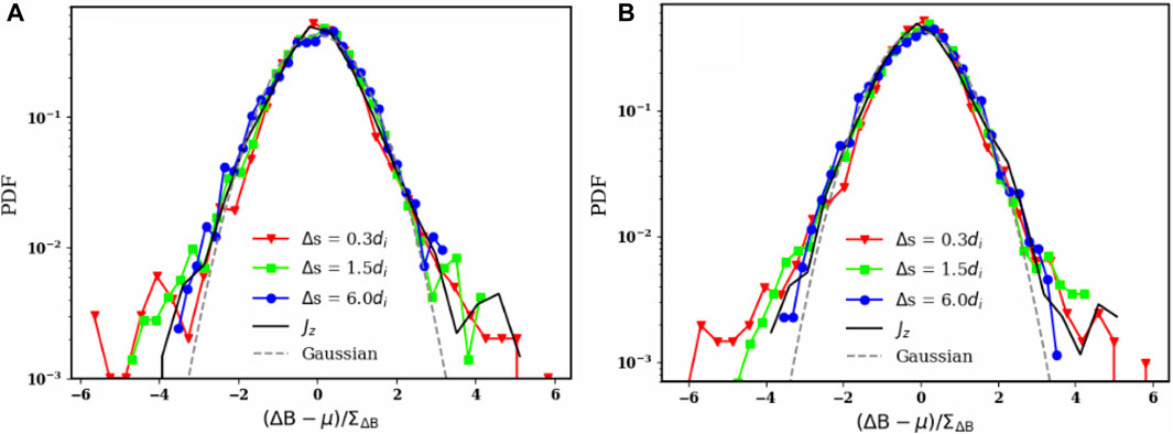
FIGURE 2. PDFs of the normalised magnetic field increments for different Δs. The curves red, green and blue correspond to the lags Δs = 0.3d_i, Δs = 1.5d_i and Δs = 6.0d_i respectively. The solid black line represents the PDF for J_z and the black dashed-line represents a Gaussian distribution. (A) statistics for 2D plane of the cross-sectional simulation. (B) statistics diagonal trajectories of the simulation.

Figure 2A, we display the statistics corresponding to the trajectories in the 2D plane of the cross-sectional simulation. On the other hand, in Figure 2B, we present the statistics corresponding to the diagonal trajectories of the simulation.

We observe a deviation from the reference Gaussian when |(ΔB − μ)/Σ_ΔB| > 2.5 for all lags considered in both case studies. Notably, a more distinct deviation from the Gaussian reference is evident for shorter lags, while longer lags (Δs = 6.0d_i, depicted in blue) show a closer resemblance to the Gaussian distribution. Specifically, the PDF for Δs = 0.3d_i exhibits heavy-tailed distributions compared to the case with Δs = 6.0d_i. It is worth mentioning that no noticeable distinction is apparent between the plots obtained for different mission sweeps.

3.2 Dependence of the PDF of the magnetic field increments on the scanning angle

To study the dependence of the PDF of the magnetic field increments on the scanning angle with respect to the background magnetic field, we compute the angle between the line connecting the spacecrafts i and j and the background magnetic field $B_0\widehat{z}$ as

$\tan {\theta }_{ij,B0}=\frac{{\rho }_{i,j}}{\mathrm{\Delta }{z}_{i,j}},(3)$

where Δz_i,j = z_i − z_j is the component of the distance parallel to $\widehat{z}$ and ${\rho }_{i,j}=\sqrt{{(x_i-x_j)}^2+{(y_i-y_j)}^2}$ is the distance perpendicular to $\widehat{z}$. Moreover, to enhance the data sample we add four additional angles θ_t = π/6, π/4, π/3, π/2 between the spacecraft configuration and $\widehat{z}$, Eq. 1 and compute

$\tilde{\theta }={\theta }_t+{\theta }_{ij,B0}.(4)$

Thus, we consider 180 different distributions of increments $f_{\mathrm{\Delta }B,ij}(\mathrm{\Delta }{s}_{ij},\tilde{\theta })$. For each distribution, there is a lag Δs_ij associated with the separation of a pair of spacecrafts and a given angle $\tilde{\theta }$. To estimate the level of intermittency, we sample the distribution f_ΔB,ij using N = 40 bins. For each bin N in the distribution we compute the difference f_ΔB,ij − f₀ between the distribution f_ΔB,ij and a standard normal distribution $f_0=e^{-{(\mathrm{\Delta }B)}^2/2\pi }$. Thus, we define the distance

$D_{ij}={⟨|f_{\mathrm{\Delta }B,ij}-f_0|⟩}_N,(5)$

where ⟨…⟩_N is the average over the total number of bins.

Figure 3A), presents the PDFs of magnetic field increment values obtained from measurements by a single-spacecraft. In this particular case, we have employed a constant lag Δs = 0.6d_i. The colour scheme in this Figure corresponds to the variation of angle within the trajectory concerning the z-axis, with sweep angles depicted as follows: 0 in black, π/6 in red, π/4 in blue, π/3 in green, and finally, π/2 in yellow. The dashed-line represents a Gaussian distribution for reference. For all angles, the PDF of the magnetic field increments shows a distinct deviation from the reference Gaussian at ∼ −2.5 and 2.5. For this lag, there is no clear dependence of the PDF of the increments on the scanning angle.

FIGURE 3

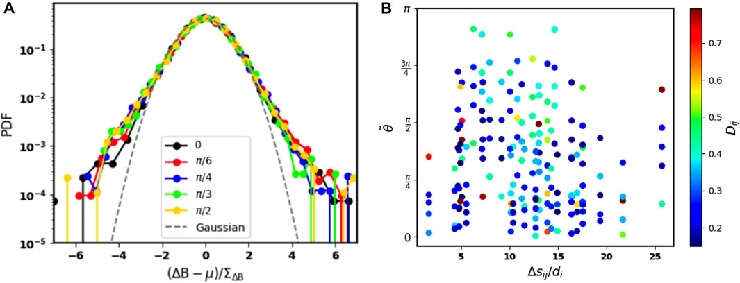
FIGURE 3. (A) PDFs of normalized magnetic field increments from a single spacecraft moving in a 1D trajectory along the simulation, with a space lag of 0.6d_i. The colours represent five scanning angles relative to the direction of the background magnetic field: 0 in black, π/6 in red, π/4 in blue, π/3 in green and π/2 in yellow. The black dashed-line represents a Gaussian reference distribution. (B) Scatter plot of the difference D_ij as a function of the lags Δs_ij and the absolute value of the angle $|\tilde{\theta }|$. The data points are colour-coded with the D_ij.

Figure 3B shows a scatter plot of D_ij as a function of the lags Δs_ij and the absolute value of the angle $|\tilde{\theta }|$, Eq. 2. The data points are colour-coded Eq. 3 from small (blue) to large (red) D_ij. This plot shows that the data points are broadly distributed in both Δs_ij and $|\tilde{\theta }|$. There is no clear correlation between D_ij and Δs_ij. Since the minimum distance between a pair of spacecrafts corresponds to a lag Δs_ij = 1.71d_i, the PDF of the magnetic increments is not expected to deviated from the Gaussian of reference, therefore the distance is D_i,j < 1 is small.

In Figure 3B there is no clear correlation between D_ij and $|\tilde{\theta }|$ which shows that there is no preferential direction parallel or perpendicular with respect to the background magnetic field.

Figure 4A depicts the Probability Distribution Function of the average single-spacecraft PVI index, Eq. 4 for five scanning angles and for a lag Δs = 0.6d_i. In this representation, the colours indicate the scanning angle of the multi-spacecraft mission relative to the z-axis, with scanning angles ranging from 0 to π/2. The distribution follows a decreasing trend and exhibits large values for low PVI thresholds. Additionally, a steeper decline is observed for PVI values exceeding 1.8. There is no clear dependence of the PDF of the single-spacecraft PVI as a function of the scanning angle for PVI < 3. Only at PVI > 3 the larger the angle, the steeper the PDF of the PVI is. However, the statistical noise is dominant for PVI > 4.

FIGURE 4

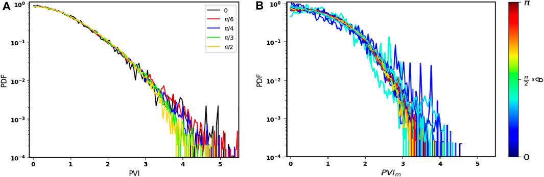
FIGURE 4. (A) PDF of the average single-spacecraft PVI for a lag Δs = 0.6d_i and for 5 different scanning angles. (B) PDF of the average multi-spacecraft PVI_m for a range of scanning angles and for a lag Δs = (7.8 − 10.2)d_i.

Figure 4B shows the Probability Distribution Function of the average multi-spacecraft PVI_m index, Eq. 5, for a range of scanning angles and for a lag Δs = (7.8–10.2)d_i. For this case, the PDF of PVI_m at small angles $\tilde{\theta }<\pi /2$ show large noise. The PDF of PVI_m shows no clear dependence with the scanning angle. Compared to the single-spacecraft PVI, the PDF of the PVI_m does not show a sustained slope. In contrast, the PDF of PVI_m decades rapidly into the range 3 < PVI_m < 4. The difference is due to the larger lag compared to the single-spacecraft case.

4 Discussion and conclusion

Figure 2 indicate a transition from a Gaussian distribution at larger scales Δs = 6.0d_i to a non-Gaussian distribution with heavy tails at smaller scales Δs = 0.3d_i. This phenomenon has already been reported in previous studies (Sorriso-Valvo et al., 1999).

Although we do not use 2D simulations, we study the 2D character of the intermittency in our simulation by taking trajectories along the plane perpendicular to the background magnetic field. Previous studies show a difference between the distribution of the increments in the 2D case compared to the 3D case (Greco et al., 2009). However, we observe no difference between the distributions for 2D trajectories and 3D trajectories crossing the entire simulation domain. This as result of the large amplitude of magnetic fluctuations in the simulation.

In Figure 3 the distributions estimated using the multi-point approach exhibit a behaviour closer to a Gaussian distribution with no tails. Moreover, the multi-point approach underestimates the level of intermittency with respect to the single-point approach. This is due to the minimum distance in the multi-spacecraft approach is larger than the scales at which the deviation from the Gaussian occurs for the single-spacecraft approach. As detailed in Table 1, the lag values that we use to sample the data in our multi-point approach span from 1.7 to 25.7 d_i, with an average of 11.7d_i. These scales are significantly larger than those sampled in the one-dimensional approach for which the non-Gaussian features show up. Thus, this approach only considers large scales, as illustrated in Figure 2, and enforces a minimum lag limited by the spacecraft separation when investigating intermittency.

The PDFs of the PVI_m multi-spacecraft Figure 4B) follow the shape of the decreasing exponential distribution. This result aligns with previous observational and simulation studies regarding the distribution of the multi-point PVI index, with the so-called kappa distribution (Chasapis et al., 2018; Pollock et al., 2018; Huang et al., 2021). However, for lower PVI values, we observe higher probabilities and a shift in the distribution’s peak compared to previous studies.

The spacecraft separation for the MMS mission is ∼ d_i, hence the effect of the intermittency is clear in the distribution of PVI_m (Chasapis et al., 2018) as well as in the distribution of the PVI for the single spacecraft, Figure 4A). In our case, for the distribution of PVI_m, since the spacecraft separation is $\sim 10d_i$ the intermittency feature is less clear. Nevertheless, our results show no clear dependence with the scanning angle. This is due to the large amplitude of the magnetic fluctuations in the simulation (δB ∼ B₀). This is not the case for the solar wind, where the amplitude of the magnetic fluctuations varies [0.1 δB ≤ B₀) (Wang et al., 2020)] and can also change as a function of heliospheric distance (Šafránková et al., 2023). Since the solar wind conditions vary depending on its origin, velocity and heliospheric distance, our results are mainly relevant to the solar wind conditions at heliospheric distances at which β ∼ 1 and populated by Alfvénic fluctuations as well as in the magnetosheath for intervals where β ∼ 1. Thus, our results can be used to study the turbulence present in the solar wind and the magnetosheath provided a data discrimination of the multi-point mission data based on the solar wind velocity. This can be applied to the upcoming Helioswarm mission.

Finally, our results contribute to the state of art multi-point analysis techniques (Broeren et al., 2021; Maruca et al., 2021; Pecora et al., 2023) and are highly relevant to the development and implementation of multi-point techniques, particularly for missions with more than 4-spacecraft in which data rapidly becomes complex and difficult to handle.

Data availability statement

Publicly available datasets were analyzed in this study. This data can be found here: https://zenodo.org/records/4313310 Three-dimensional magnetic reconnection in particle-in-cell simulations of anisotropic plasma turbulence (Simulation Data).

Author contributions

AG: Conceptualization, Data curation, Formal Analysis, Investigation, Methodology, Writing–original draft. JA: Conceptualization, Data curation, Formal Analysis, Investigation, Methodology, Writing–original draft. SV: Conceptualization, Data curation, Formal Analysis, Investigation, Methodology, Writing–original draft.

Funding

The author(s) declare financial support was received for the research, authorship, and/or publication of this article. JA is supported by NASA grant 80NSSC21K2048 and NSF grant 2142430.

Acknowledgments

We acknowledge the Beyond Research program from Facultad de Ciencias, Universidad Nacional de Colombia.

Conflict of interest

The authors declare that the research was conducted in the absence of any commercial or financial relationships that could be construed as a potential conflict of interest.

Publisher’s note

All claims expressed in this article are solely those of the authors and do not necessarily represent those of their affiliated organizations, or those of the publisher, the editors and the reviewers. Any product that may be evaluated in this article, or claim that may be made by its manufacturer, is not guaranteed or endorsed by the publisher.

References

Agudelo Rueda, J. A., Verscharen, D., Wicks, R. T., Owen, C. J., Nicolaou, G., Walsh, A. P., et al. (2021). Three-dimensional magnetic reconnection in particle-in-cell simulations of anisotropic plasma turbulence. J. Plasma Phys. 87, 905870228. doi:10.1017/s0022377821000404

CrossRef Full Text | Google Scholar

Broeren, T., Klein, K., TenBarge, J., Dors, I., Roberts, O., and Verscharen, D. (2021). Magnetic field reconstruction for a realistic multi-point, multi-scale spacecraft observatory. Front. Astronomy Space Sci. 8, 727076. doi:10.3389/fspas.2021.727076

CrossRef Full Text | Google Scholar

Bruno, R. (2019). Intermittency in solar wind turbulence from fluid to kinetic scales. Earth Space Sci. 6, 656–672. doi:10.1029/2018EA000535

CrossRef Full Text | Google Scholar

Chasapis, A., Matthaeus, W. H., Parashar, T. N., Wan, M., Haggerty, C. C., Pollock, C. J., et al. (2018). In situ observation of intermittent dissipation at kinetic scales in the earth’s magnetosheath. Astrophysical J. Lett. 856, L19. doi:10.3847/2041-8213/aaadf8

CrossRef Full Text | Google Scholar

Chasapis, A., Retinò, A., Sahraoui, F., Canu, P., Vaivads, A., Khotyaintsev, Y. V., et al. (2015). Thin current sheets and associated electron heating in turbulent space plasma. Astrophysical J. Lett. 804, L1. doi:10.1088/2041-8205/804/1/L1

CrossRef Full Text | Google Scholar

Chhiber, R., Chasapis, A., Bandyopadhyay, R., Parashar, T., Matthaeus, W. H., Maruca, B., et al. (2018). Higher-order turbulence statistics in the earth’s magnetosheath and the solar wind using magnetospheric multiscale observations. J. Geophys. Res. Space Phys. 123, 9941–9954. doi:10.1029/2018ja025768

CrossRef Full Text | Google Scholar

Dong, S., Huang, Y., Yuan, X., and Lozano-Durán, A. (2020). The coherent structure of the kinetic energy transfer in shear turbulence.

Google Scholar

Goldstein, M., Roberts, D., and Fitch, C. (1994). Properties of the fluctuating magnetic helicity in the inertial and dissipation ranges of solar wind turbulence. J. Geophys. Res. Space Phys. 99, 11519–11538. doi:10.1029/94ja00789

CrossRef Full Text | Google Scholar

Gosling, J. T. (2014). “The solar wind,” in Encyclopedia of the solar system (Elsevier), 261–279.

CrossRef Full Text | Google Scholar

Greco, A., Chuychai, P., Matthaeus, W. H., Servidio, S., and Dmitruk, P. (2008). Intermittent mhd structures and classical discontinuities. Geophys. Res. Lett. 35. doi:10.1029/2008GL035454

CrossRef Full Text | Google Scholar

Greco, A., Matthaeus, W. H., Perri, S., Osman, K. T., Servidio, S., Wan, M., et al. (2018). Partial variance of increments method in solar wind observations and plasma simulations. Wind Observations Plasma Simulations 214, 1. doi:10.1007/s11214-017-0435-8

CrossRef Full Text | Google Scholar

Greco, A., Matthaeus, W. H., Servidio, S., Chuychai, P., and Dmitruk, P. (2009). Statistical analysis of discontinuities in solar wind ace data and comparison with intermittent mhd turbulence. Astrophysical J. 691, L111–L114. doi:10.1088/0004-637X/691/2/L111

CrossRef Full Text | Google Scholar

Huang, S., Zhang, J., Yuan, Z., Jiang, K., Wei, Y., Xu, S., et al. (2021). Intermittent dissipation at kinetic scales in the turbulent reconnection outflow. Geophys. Res. Lett. 49. doi:10.1029/2021GL096403

CrossRef Full Text | Google Scholar

Klein, K. G., Spence, H., Alexandrova, O., Argall, M., Arzamasskiy, L., Bookbinder, J., et al. (2023). Helioswarm: a multipoint, multiscale mission to characterize turbulence. arXiv preprint arXiv:2306.06537.

Google Scholar

Livadiotis, G., and McComas, D. (2013). Understanding kappa distributions: a toolbox for space science and astrophysics. Space Sci. Rev. 175, 183–214. doi:10.1007/s11214-013-9982-9

CrossRef Full Text | Google Scholar

Marsch, E., Mühlhäuser, K.-H., Schwenn, R., Rosenbauer, H., Pilipp, W., and Neubauer, F. (1982). Solar wind protons: Three-dimensional velocity distributions and derived plasma parameters measured between 0.3 and 1 au. J. Geophys. Res. Space Phys. 87, 52–72. doi:10.1029/ja087ia01p00052

CrossRef Full Text | Google Scholar

Maruca, B. A., Agudelo Rueda, J. A., Bandyopadhyay, R., Bianco, F. B., Chasapis, A., Chhiber, R., et al. (2021). Magnetore: mapping the 3-d magnetic structure of the solar wind using a large constellation of nanosatellites. Front. astronomy space Sci. 8, 665885. doi:10.3389/fspas.2021.665885

CrossRef Full Text | Google Scholar

Palacios, J. C., Bourouaine, S., and Perez, J. C. (2022). On the statistics of elsasser increments in solar wind and magnetohydrodynamic turbulence. Astrophysical J. Lett. 940, L20. doi:10.3847/2041-8213/ac92f6

CrossRef Full Text | Google Scholar

Pecora, F., Servidio, S., Primavera, L., Greco, A., Yang, Y., and Matthaeus, W. H. (2023). Multipoint turbulence analysis with helioswarm. Astrophysical J. Lett. 945, L20. doi:10.3847/2041-8213/acbb03

CrossRef Full Text | Google Scholar

Perrone, D., Alexandrova, O., Roberts, O. W., Lion, S., Lacombe, C., Walsh, A., et al. (2017). Coherent structures at ion scales in fast solar wind: cluster observations. Astrophysical J. 849, 49. doi:10.3847/1538-4357/aa9022

CrossRef Full Text | Google Scholar

Plice, L., Perez, A. D., and West, S. (2019). Helioswarm: swarm mission design in high altitude orbit for heliophysics.

Google Scholar

Pollock, C., Burch, J., Chasapis, A., Giles, B., Mackler, D., Matthaeus, W., et al. (2018). Magnetospheric multiscale observations of turbulent magnetic and electron velocity fluctuations in earth’s magnetosheath downstream of a quasi-parallel bow shock. J. Atmos. Solar-Terrestrial Phys. 177, 84–91. doi:10.1016/j.jastp.2017.12.006

CrossRef Full Text | Google Scholar

Šafránková, J., Němeček, Z., Němec, F., Verscharen, D., Horbury, T. S., Bale, S. D., et al. (2023). Evolution of magnetic field fluctuations and their spectral properties within the heliosphere: statistical approach. Astrophysical J. Lett. 946, L44. doi:10.3847/2041-8213/acc531

CrossRef Full Text | Google Scholar

Sorriso-Valvo, L., Carbone, V., Veltri, P., Consolini, G., and Bruno, R. (1999). Intermittency in the solar wind turbulence through probability distribution functions of fluctuations. Geophys. Res. Lett. 26, 1801–1804. doi:10.1029/1999GL900270

CrossRef Full Text | Google Scholar

Taylor, G. I. (1938). The spectrum of turbulence. Proc. R. Soc. Lond. Ser. A-Mathematical Phys. Sci. 164, 476–490. doi:10.1098/rspa.1938.0032

CrossRef Full Text | Google Scholar

Wang, X., Tu, C., and He, J. (2020). Fluctuation amplitudes of magnetic-field directional turnings and magnetic-velocity alignment structures in the solar wind. Astrophysical J. 903, 72. doi:10.3847/1538-4357/abb883

CrossRef Full Text | Google Scholar

Wu, P., Perri, S., Osman, K., Wan, M., Matthaeus, W., Shay, M., et al. (2013). Intermittent heating in solar wind and kinetic simulations. Astrophysical J. Lett. 763, L30. doi:10.1088/2041-8205/763/2/l30

CrossRef Full Text | Google Scholar

Yordanova, E., Vörös, Z., Varsani, A., Graham, D. B., Norgren, C., Khotyaintsev, Y. V., et al. (2016). Electron scale structures and magnetic reconnection signatures in the turbulent magnetosheath. Geophys. Res. Lett. 43, 5969–5978. doi:10.1002/2016gl069191

CrossRef Full Text | Google Scholar