GOLD plasma bubble observations comparison with geolocation of plasma irregularities by back propagation of the high-rate FORMOSA7/COSMIC 2 scintillation data

Introduction

Using the FORMOSA7/COSMIC 2 (F7/C2) mission (Anthes and Schreiner, 2019; Yue et al., 2014) GNSS high-rate phase and amplitude data and back-propagation method (Sokolovskiy et al., 2002), we geolocate plasma irregularities that cause scintillations (below we call this geolocation of scintillation for brevity). In the equatorial region, the scintillations are often associated with the plasma bubbles. Plasma bubbles are caused by the Rayleigh-Tayler (R-T) instability on the bottom side of the ionosphere [e.g., Sultan, 1996; Wu, 2015; 2017]. As bubble occurs, the ionosphere develops elongated depletions along the magnetic field lines during the post-sunset hours. The pre-reversal enhancement of the vertical ion drift can lead to positive growth rate of the R-T instability [e.g., Sultan 1996; Wu, 2015]. Inside the bubbles, which have scales hundreds of kilometers, the smaller-scale irregularities develop. These irregularities with scales of order of 1 km or less are responsible for the scintillation localizable by back propagation. Thus, the geolocation method detects the small-scale plasma irregularities in the bubble, not the bubble itself. This space weather application has a great value as the ionospheric scintillation which affects GNSS signals can greatly disrupt the GNSS and other radio communication systems potentially causing great economical losses.

The US-Taiwan joint mission F2/C2 has six equatorial orbiting satellites and was launched into space on 25 June 2019. All six satellites carry GNSS receivers called Tri-GNSS Radio Occulation System (TGRS) (Tien et al., 2012). The TGRS instruments have an on-board trigger mechanism to transmit high-rate (100 Hz for GLONASS and 50 Hz for GPS) phase and amplitude data (later stored in the scnPhs files) to the ground. The trigger is activated by the on-board GNSS signal S4 value greater than 0.1. By applying the back propagation method to the data from scnPhs files, the F7/C2 team has been producing geolocation of scintillations on a routine basis. In the past, when the S4 value from GNSS RO missions were analyzed, the scintillation was often assigned to the tangent point, which is not true most of the time. The back-propagation method derived geolocation of the scintillation are more accurate compared to using the tangent point. Moreover, the F7/C2 can provide geolocation around the globe.

Because of the strong connection between the scintillation and plasma bubbles, we can assume that bubbles and scintillations are co-located in most of the cases. Detecting and locating bubbles is not easy. Ground based all sky cameras can capture bubbles [e.g., Okoh et al., 2017] as depletions in the O 630 nm redline emission. But they have very limited coverage and are affected by weather conditions. Satellite UV imagers can also detect bubbles in the O 135.6 nm emission, which is proportional to the ion density squared. In the past, most of satellite UV imaging detectors were on high inclination orbits such as TIMED GUVI and DMSP SSUSI instrument (Comberiate and Paxton, 2010). The NASA mission GOLD UV imager (Eastes et al., 2017; Eastes et al., 2020) on board a geosynchronous orbit is the first to provide continuous coverage over the American sector and has frequently observed bubbles in the night time data.

Because the F7/C2 back propagation geolocation data will be used for operational purposes, a validation is needed. That can be accomplished by using bubble detection to locate the source of the scintillation and compare with the geolocation results. The GOLD UV bubble images become a logical choice to for this purpose in the American sector. The first step is to develop an algorithm to the determine the bubble locations based on the GOLD UV images.

In this paper, we describe a GOLD UV image bubble location algorithm and comparison with the geolocation. We will discuss the results of validation of the F7/C2 geolocation product and summarize our findings.

GOLD bubble analysis method

GOLD is a NASA mission of UV imager on a geo-synchronous satellite over the American sector (47.5W) [e.g., Eastes et al., 2017; 2020]. The GOLD images cover the American sector, we used the nighttime mode data, which is taken after dusk. We use intensity of the O 135.6 nm emission line in the GOLD UV spectra. Bubbles are often seen in the images.

The GOLD instrument has two identical channels A and B, when the solar terminator just across Africa, channel B is used to do both northern and southern hemisphere for the night mode observation. The northern and southern scan each lasts about 15 min. Hence the combined north and south scan lasts about 30 min. As the solar terminator reaches the American continent, both Channel A and B are used for the night mode observation. Channel A for the northern and B for the southern hemisphere. Because of using two channels, the combined north and south scan lasts only 15 min.

To determine the bubble locations in the magnetic longitude, we bin the GOLD image pixels in 1-degree magnetic longitudinal grids from 25° magnetic north to the magnetic equator. We bin the pixels from the magnetic equator to 25° south for the southern hemisphere with the same magnetic longitudinal grid. Figure 1 shows an example of the binning pattern for the northern (lime) and southern (magenta) hemispheres and GOLD image of plasma bubbles identified. In this way, we have a northern and southern track of binned magnetic longitudinal variation of the UV 135.6 nm emission. To locate bubbles, we search all minimum values in both the northern and southern tracks of the binned GOLD UV 135.6 nm emission (see Figure 2). We should expect the bubbles coincide with the minima in the UV emission. To reduce false positive bubble identifications, we compare the minimum locations in both the northern and southern tracks, if we cannot find minimum within 2 degrees of magnetic longitude in both tracks, we will not flag the minimum as a bubble location. Another reason for comparing the northern and southern track is to ensure the depletion remain roughly in the same magnetic longitude. Because GOLD image is a 2D projection of a 3D ionosphere with plasma bubbles, the depletion from the bubble in the GOLD image may deviate from the same magnetic longitude. If that is case, our selection criterion will not select the bubble for comparison with geolocation. If we find both northern and southern bubbles, then we pick the northern location for the bubble. Figure 2 shows the nine minima in northern and all nine have companion minima in the southern hemisphere and they are selected as shown in the figure. The locations are plotted on GOLD image in Figure 1.

Figure 1

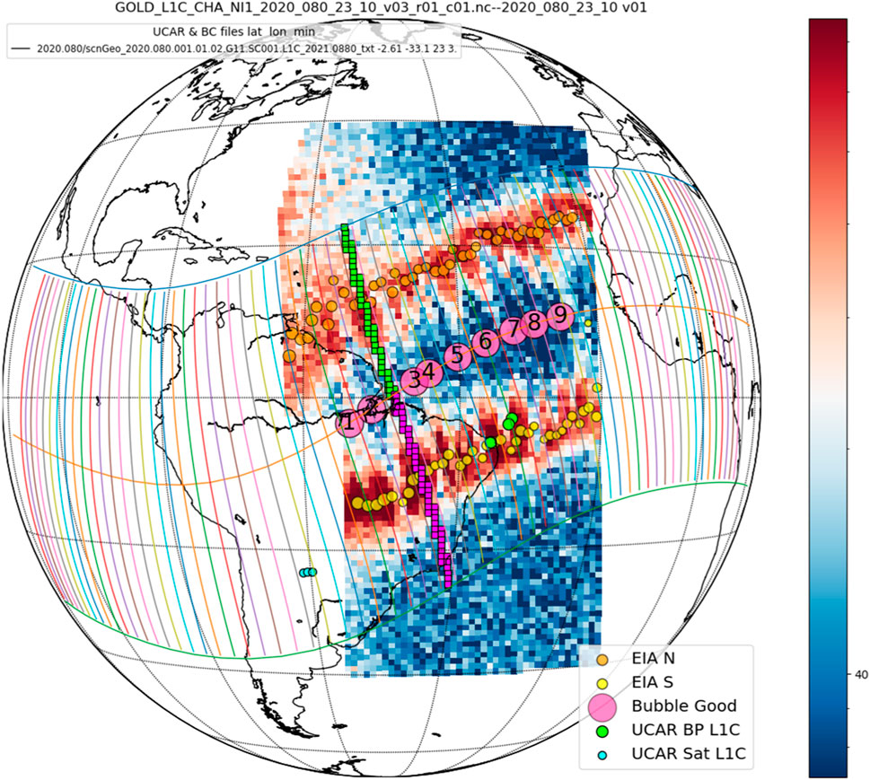
Figure 1. Example of GOLD Image of Bubbles with the F7/C2 Geolocations of the Scintillations. The equatorial ionosphere anomalies are also plotted (EIA N, S, orange and yellow circles). Bubbles are plotted at the magnetic equator (magenta cycles). F7/C2 locations (UCAR Sat L1C, cyan circles) and scintillation geolocation (UCAR BP L1C, green circles) are shown. The GOLD image binning pattern for the northern (lime squares) and southern (magenta squares) hemisphere within a 1-degree grid are displayed.

Figure 2

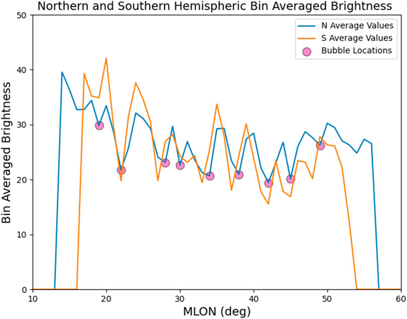
Figure 2. The GOLD UV brightness averaged within 1° magnetic longitude grid between 0 and 25 MLAT (north, blue color) and 0 to −25 MLAT (south, orange color). Selected bubble locations at northern UV brightness minima (with southern companions with in 2 degree of MLON). The nine bubbles are also plotted in Figure 1.

We also estimate the depth and width of the bubbles. The key to estimate these depth and width is to calculate the baseline for a non-disturbed condition. We used a polynomial fit of the binned UV longitudinal variation of the northern and southern tracks. Because the existing bubbles, the fitted curves will be lower than an ideal baseline. To address this issue with a simple algorithm, we remove the binned UV data below the fitted curve, then use the remaining UV data points above the first fitting curve to do another polynomial fit along the magnetic longitude. The second fit will be much closer to the ideal baseline. We then use that as the baseline in our analysis. The same procedure is used for both northern and southern tracks. To estimate the width of the bubble, we pick the separation of the half way points between the bottom of bubble and the baseline. We will use the larger of the northern and southern bubble width for the bubble width. The deeper depth of the two will be used to represent bubble depth.

While this method can automatically determine bubble locations when the UV emission is strong and bubble depletion contrast is clear, we still have cases, where the bubbles are not apparent in the GOLD images. To ensure no falsely identified bubbles are used in analysis, we used visual inspection of the GOLD images to confirm the automatic search results. The visual inspection is performed by a group of people to reduce bias.

Back propagation method

Back propagation (BP) method has been used to geolocate the scintillation based on the GNSS high-rate phase and amplitude data (Sokolovskiy et al., 2002). The method is based on several assumptions. First, plasma irregularities must occupy limited volume so that wave propagation is considered in the phase screen approximation. In other words, radio waves undergo only phase fluctuations inside the volume. Amplitude fluctuations (observed along receiver trajectory which crosses the direction of wave propagation) develop after propagation through the volume and increase with the distance from the volume due to focusing/defocusing effects caused by the phase fluctuations induced by plasma irregularities. The phase and amplitude measured by the receiver in orbit can be used as the boundary condition for solving wave equation in a vacuum and reconstruction of the phase and amplitude fluctuations back from transmitter to receiver. Amplitude fluctuations decrease from receiver to the region with irregularities and then increase again due to imaginary focusing/defocusing. Thus, the region of minimum amplitude fluctuations traces the region with irregularities. Second, irregularities must be anisotropic (elongated) to reduce wave propagation problem from three to two dimensions. This is needed because the phase and amplitude are measured on 1-dimensional receiver trajectory which is insufficient for solving 3-dimensional wave propagation problem. Third, direction of irregularities must be known for orientation of the BP plane. In the equatorial F region plasma irregularities are aligned with the magnetic field lines which allows to use the magnetic field model (IGRF-13) for orientation of the BP plane. Compared to (Sokolovskiy et al., 2002), the BP method was fully automated and further enhancements improving geolocation accuracy were included (this will be discussed in a separate publication).

In this study, we applied BP in 10-s intervals. This is the trade-off between two conditions: (i) the scanned volume must be large enough to include multiple irregularities which cause scintillation (to reduce the boundary effects in BP) and (ii) must be small enough so that statistical structure of the irregularities must not be substantially different inside the volume. Both (i) and (ii) are required for a more reliable estimation of the distance to minimum of amplitude scintillation by BP.

Comparison of the bubble location and scintillation geolocation

We selected the time period from Day 044–106 in 2020 for the GOLD bubble and F7/C2 scnPhs file geolocation comparison. The selection of the time is associated with F7/C2 calibration/validation of other instruments and mostly coincides with the bubble active period in the American sector.

Figure 1 not only shows the GOLD UV image with bubbles, but also F7/C2 geolocated scintillations. In the figure we also located north and south equatorial ionosphere anomaly (EIA). Since the GOLD bubble has time cadence of 30 min or 15 min, the F2/C2 geolocation (based on 10-s data intervals) can have multiple overlaps with the same GOLD images. We will associate the geolocation with the GOLD bubble that is closest in magnetic longitude to the geolocation. If the geolocation is within the width of the GOLD bubble, then we label that as zero difference. If it is outside the GOLD bubble width, then the distance from edge of the bubble to the geolocation will be assigned as the longitudinal difference. In the case shown in Figure 1, we have three geolocations from one scnPhs file (green circles). The F7/C2 satellite locations are on the west (cyan circles). The scnPhs file data are from the forward POD antenna facing east. Two geolocations on the east, will be associated with bubble # 6, whereas the one on the west will be linked to bubble # 5. UCAR geolocation has the tendency to pick the scintillation near the EIAs as shown in this case. Because both northern and southern hemisphere GOLD data are used, if only one hemisphere data is available, no bubbles will be picked at that magnetic longitude. In Figure 1, there could be a bubble beyond bubble # nine on the east, which was not picked because of missing the southern hemisphere data as shown in Figure 2 the southern hemisphere brightness data end earlier compared to the northern track.

Before the comparison, we inspected all GOLD images with geolocations overplotted on top. The geolocations that are on the edge of GOLD UV image data or do not intersect with the bubbles were removed. A total of 8 GLONASS and 10 GPS scnPhs files were removed for these reasons. A total of 84 GLONASS and 63 GPS scnPhs files are used for our comparison. Out of these scnPhs files we have 479 GLONASS and 366 GPS geolocations based on 10-s intervals.

Figure 3 shows the GOLD bubble magnetic longitudes vs. the F7/C2 geolocation scintillation longitudes. There is a general good agreement between the bubble locations vs. geolocation of scintillations for both GLONASS and GPS. To be more quantitative of the zonal difference, the distribution is plotted in Figure 4. The numerical distributions of zonal difference are listed in Table 1. The RMS of the distribution is 1.57 deg and mean is 0.13 of the distribution.

Figure 3

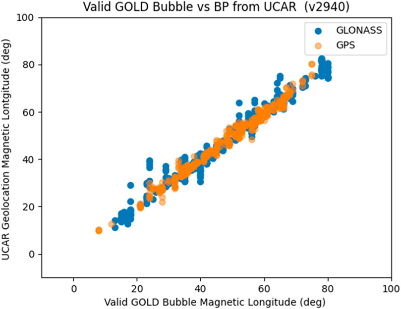
Figure 3. The GOLD bubble magnetic longitudes vs. that of the geolocations from GLONASS (blue) and GPS (orange) L1 signals.

Figure 4

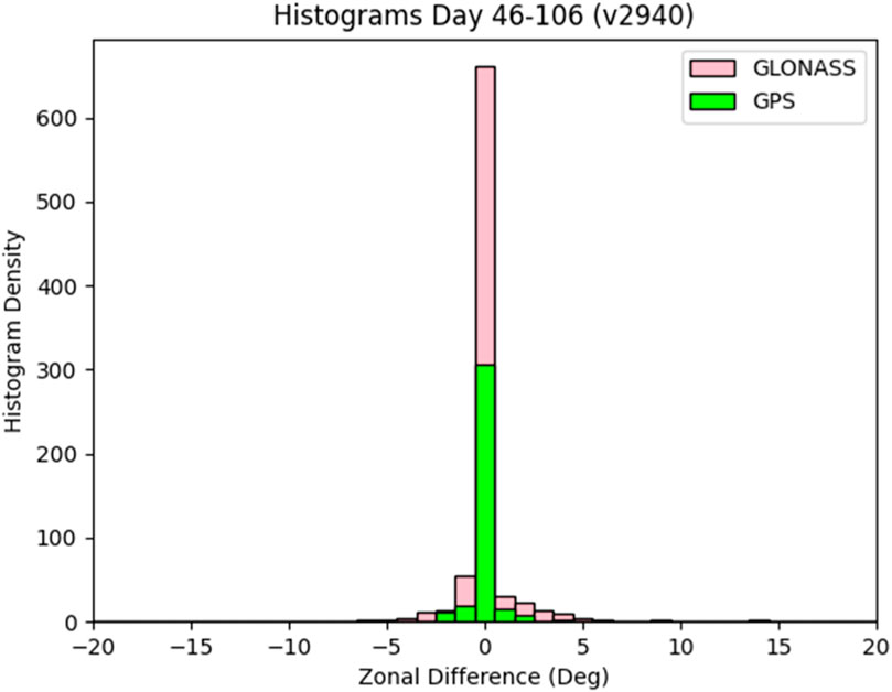
Figure 4. Zonal difference distribution between the GOLD bubble and F7/C2 geolocation scintillation. GLONASS and GPS are in different colors.

Table 1

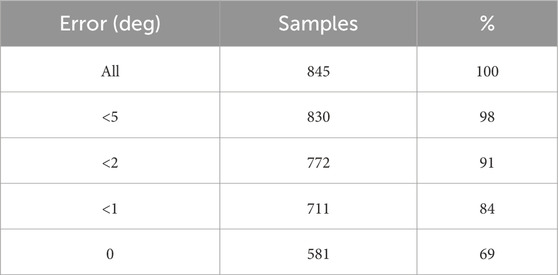
Table 1. GOLD bubble and F7/C2 geolocation zonal difference distribution.

There are 15 geolocations from seven scnPhs files with zonal differences larger than 5° in magnetic longitude. After a close examination of GOLD images, we determined that in those cases, the GOLD image either show weak structures which were not selected by visual inspection or the GOLD images have poor contrast. In other words, the GOLD data in those cases did not provide good references for comparison. The images may be selected because there are other selected GOLD bubbles. Compared to the total number of the geolocations, the number of outliers is small.

We have many multiple bubble cases as shown in Figure 1. We would like to see how the geolocation performs in single bubble intersection cases. A total of eight scnPhs files with 54 geolocations were selected for this zonal difference analysis. The distribution is shown in Figure 5 and the same statistical values are listed in Table 2. The RMS for the differences is 0.45 deg in magnetic longitude and mean value difference is 0.00. That shows in the case of single intersection the geolocation can be accurate up to half degree in longitude (∼50 km). There are no outliers for the single intersection case.

Figure 5

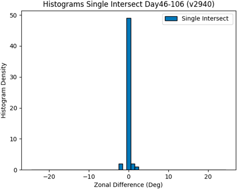
Figure 5. Zonal difference distribution between GOLD bubble and F7/C2 geolocation scintillation for single intersection cases.

Table 2

Table 2. Zonal difference statistics between GOLD bubble and F7/C2 scintillation for single intersection cases.

The zonal difference dependences on the scintillation altitude, local time, geolocation distance, and GNSS signal SNR are plotted in Figure 6. We do not see a clear trend of the zonal difference vs. these parameters. That implies that the geolocation method should work well over these parameter ranges. Finally, the scintillation altitude and local time distribution are plotted in Figure 7. As the ionospheric density gradually decreases moving into the night, we see fewer scintillations at high altitude. We have a cutoff at 600 km for geolocations. Also the GOLD observations do not extend deep into the night due to low UV emissions. Most of the bubbles occur near dusk after sunset, which is why we see more geolocations before 22 LT.

Figure 6

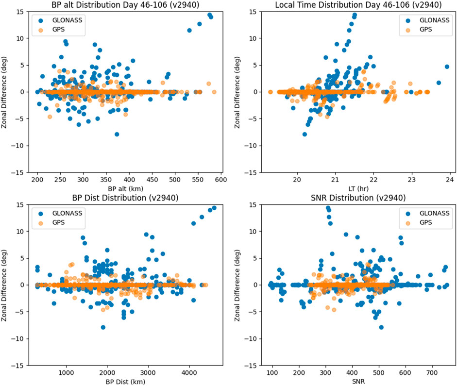
Figure 6. Zonal difference vs. altitude (upper left), local time (upper right), geolocation distance (lower left), and SNR (Signal to Noise Ratio) of the GNSS signals (lower right).

Figure 7

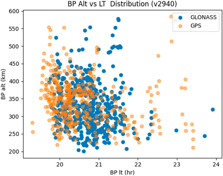
Figure 7. F7/C2 geolocation of the scintillation altitude and local time distribution.

Discussion

The scnPhs files (including high rate phase and amplitude data and orbits) along with the scnGeo files including geolocation results (coordinates of the localized irregularities for those 10-s intervals with successful BP) are new products from F7/C2. In this analysis, we only used results obtained with GLONASS and GPS L1 signals. Taking advantage of the availability of the GOLD UV image data, we were able to show a good agreement between the F7/C geolocation and the GOLD bubble locations. This suggests that the scintillations selected in the local time interval in the GNSS signals are mostly caused by the plasma bubbles. In the cases with multiple bubbles, the overall statistics show the zonal difference RMS of about 1.5°, whereas the single intersection cases have about 0.5° RMS (∼55 km) zonal difference. Since we used 10 s intervals (maximum ∼70 km of the ray cross track) for the BP method, the 70 km may be considered the spatial resolution of geolocation. The RMS of the zonal difference is consistent with the spatial resolution of the BP method. Note that the minimum separation from GOLD image neighboring bubble is 2° in case we have multiple bubbles. That is not to say we have multi-bubbles all the time and the GOLD bubble location and COSMIC geolocation separation can be larger than 2° as shown in the statistical results.

The results also show the robustness of the geolocation method, as we did not see many outliers in our comparison. Geolocation will greatly improve our statistics of bubble occurrence compared to past COSMIC GNSS S4 based analysis [e.g., Wu et al., 2021]. That will help to track down possible trigger mechanism by pin-pointing the scintillation locations. Another useful information from the geolocation files is altitude of the scintillation. While we did not analyze the altitude in this study, the altitude information may help characterizing the bubble evolution.

The GOLD bubble location algorithm also works well. When the GOLD quality is good, the method can determine the bubbles in GOLD images very accurately. The north and south track comparison helps to reduce false positive for bubble location. Overall, the F7/C2 scnPhs file based geolocation will be an important space weather product. It will pin point the scintillations at regions, where the observational coverage has been lacking.

Summary

1. F7/C2 high rate scnPhs files enable the back-propagation method to geolocate the scintillations at all longitudes for accurate scintillation locations.

2. Comparison with GOLD bubble locations show a good agreement between the geolocation of scintillation and the bubble locations. The zonal difference is about 1.5 deg in magnetic longitude for all cases and 0.5 deg for single intersection cases.

3. The GOLD bubble location determine method provides accurate bubble information.

Data availability statement

The raw data supporting the conclusion of this article will be made available by the authors, without undue reservation.

Author contributions

QW: Writing–original draft, Writing–review and editing. JB: Investigation, Writing–review and editing. SS: Investigation, Methodology, Software, Writing–review and editing. WS: Investigation, Writing–review and editing. NP: Investigation, Writing–review and editing. J-PW: Investigation, Writing–review and editing. IC: Investigation, Writing–review and editing. IZ: Investigation, Writing–review and editing.

Funding

The author(s) declare that financial support was received for the research, authorship, and/or publication of this article. This research is supported by the following grants. This work was supported by Air Force Contract FA8803-19-C-0004. National Center for Atmospheric Research is supported by the National Science Foundation corporative agreement 1852977 and grants AGS-2054356 AGS-2120511 and NASA grants 80NSSC20K0199, NNX17AG69G, 20-GIGI20-007.

Acknowledgments

The GOLD nighttime data are available from https://gold.cs.ucf.edu/data/search/. The F7/C2 geolocation data used in this study are available upon request.

Conflict of interest

The authors declare that the research was conducted in the absence of any commercial or financial relationships that could be construed as a potential conflict of interest.

Publisher’s note

All claims expressed in this article are solely those of the authors and do not necessarily represent those of their affiliated organizations, or those of the publisher, the editors and the reviewers. Any product that may be evaluated in this article, or claim that may be made by its manufacturer, is not guaranteed or endorsed by the publisher.

References

Anthes, R. A., and Schreiner, W. S. (2019). Six new satellites watch the atmosphere over Earth’s equator. Eos Wash(. DC) 100. doi:10.1029/2019EO131779

CrossRef Full Text | Google Scholar

Comberiate, J., and Paxton, L. J. (2010). Coordinated UV imaging of equatorial plasma bubbles using TIMED/GUVI and DMSP/SSUSI. Space weather. 8, S10002. doi:10.1029/2009SW000546

CrossRef Full Text | Google Scholar

Eastes, R. W., McClintock, W. E., Burns, A. G., Anderson, D. N., Andersson, L., Aryal, S., et al. (2020). Initial observations by the GOLD mission. J. Geophys. Res. Space Phys. 125, e2020JA027823. doi:10.1029/2020JA027823

CrossRef Full Text | Google Scholar

Eastes, R. W., McClintock, W. E., Burns, A. G., Anderson, D. N., Andersson, L., Codrescu, M., et al. (2017). The global-scale observations of the limb and disk (GOLD) mission. Space Sci. Rev. 212 (1-2), 383–408. doi:10.1007/s11214-017-0392-2

CrossRef Full Text | Google Scholar

Okoh, D., Rabiu, B., Shiokawa, K., Otsuka, Y., Segun, B., Falayi, E., et al. (2017). First study on the occurrence frequency of equatorial plasma bubbles over West Africa using an all-sky airglow imager and GNSS receivers. J. Geophys. Res. Space Phys. 122 (12), 430. doi:10.1002/2017JA024602

CrossRef Full Text | Google Scholar

Sokolovskiy, S., Schreiner, W., Rocken, C., and Hunt, D. (2002). Detection of high-altitude ionospheric irregularities with GPS/MET. Geophys. Res. Lett. 29 (3). doi:10.1029/2001GL013398

CrossRef Full Text | Google Scholar

Sultan, P. J. (1996). Linear theory and modeling of the Rayleigh-Taylor instability leading to the occurrence of the equatorial spread F. J. Geophys Res. 101 (26), 875–926. doi:10.1029/96JA00682

CrossRef Full Text | Google Scholar

Tien, J. Y., Okihiro, B. B., Esterhuizen, S. X., Franklin, G. W., Meehan, T. K., Munson, T. N., et al. (2012). “Next generation scalable space-borne GNSS science receiver,” in Proc. 2012 int. tech. meet. inst. navig., Newport Beach, CA, September 17 - 21, 2012, 882–914.

Google Scholar

Wu, Q. (2015). Longitudinal and seasonal variation of the equatorial flux tube integrated Rayleigh-Taylor instability growth rate. J. Geophys. Res. Space Phys. 120. doi:10.1002/2015JA021553-T

CrossRef Full Text | Google Scholar

Wu, Q. (2017). Solar effect on the Rayleigh-Taylor instability growth rate as simulated by the NCAR TIEGCM. J. Atmos. Solar-Terrestrial Phys. 156, 97–102. doi:10.1016/j.jastp.2017.03.007

CrossRef Full Text | Google Scholar

Wu, Q., Chou, M. Y., Schreiner, W., Braun, J., Pedatell, N., and Cherniak, I. (2021). COSMIC observation of stratospheric gravity wave and ionospheric scintillation correlation. J. Atmos. Solar-terrestrial Phys. 217, 105598. doi:10.1016/j.jastp.2021.105598

CrossRef Full Text | Google Scholar

Yue, X., Schreiner, W. S., Pedatella, N., Anthes, R. A., Mannucci, A. J., Straus, P. R., et al. (2014). Space weather observations by GNSS radio occultation: from FORMOSAT-3/COSMIC to FORMOSAT-7/COSMIC-2. Weather 12 (11), 616–621. doi:10.1002/2014SW001133

PubMed Abstract | CrossRef Full Text | Google Scholar