Simulated cusp ion dispersions and the day-side magnetopause reconnection rate

When the interplanetary magnetic field (IMF) is southward dominant, antiparallel day-side magnetic reconnection occurs near the equatorial magnetopause, and the reconnection rate quantifies how much magnetic flux is removed from the magnetosphere per time. During space weather events, this is a key quantity to understand, because the day-side magnetopause can be significantly eroded, potentially receding within geosynchronous orbit. However, direct observations of the reconnection rate are challenging, so attempts have been made to quantify the reconnection rate through remote measurements. In particular, ion dispersions observed in the low-altitude cusp have been connected to the day-side magnetopause reconnection rate, assuming the dispersions are formed by time-of-flight differences for different energy particles convecting with the same field line. This provides a promising avenue to probe the day-side reconnection rate with satellites that pass through the low-altitude cusp, like Defense Meteorological Satellite Program (DMSP) and Tandem Reconnection and Cusp Electrodynamics Reconnaissance Satellites (TRACERS). In this study, cusp ion dispersion signatures are constructed using the forward particle tracing capability of the GAMERA-CHIMP global magnetohydrodynamics (MHD) with test particle framework. Under idealized solar wind driving with steady southward IMF, the reconnection rate is calculated and compared with an independent measure of the reconnection rate based on the amount of magnetospheric flux reconnected per time. Changes in magnetospheric flux content indicate the day-side magnetopause reconnection rate is $\sim 0.65$ mV/m with variations up to 0.2 mV/m occurring on a $\sim 5$ minute timescale which are associated with the formation and evolution of magnetic flux ropes. Reconnection rates calculated from simulated cusp ion dispersions are mostly in the range 0.2–1.4 mV/m. These values corresponding to idealized solar wind driving conditions provide a benchmark for future case studies. Ultimately, the goal of this study is to demonstrate how the reconnection rate can be calculated from simulated cusp ion dispersions.

1 Introduction

Spacecraft flying along the direction of flux tube motion in the low-altitude cusp observe ion time-energy dispersion due to particle entry at the day-side magnetopause and global convection of cusp magnetic field lines. In the case of steady southward interplanetary magnetic field (IMF) orientation, a newly reconnected day-side magnetic field line convects away from the mostly equatorial x-line towards either the northern or southern cusp. This magnetic field line convection mapped to the ionosphere corresponds to motion from low-to-high magnetic latitude (MLat). Faster particles will reach a given altitude in less time than slower particles, so a spacecraft crossing through the cusp will observe higher energy particles on cusp magnetic field lines mapping closer to the x-line (lower magnetic latitude).

Slopes of cusp ion dispersions contain information about the rate of magnetic reconnection on the day-side magnetopause (Lockwood and Smith, 1992). It is noteworthy that the low-altitude cusp can be used to remote sense the day-side magnetopause reconnection rate, because it is far easier to access the low-altitude cusp than the magnetopause x-line. Spacecraft which repeatedly pass through the cusp, like Tandem Reconnection and Cusp Electrodynamics Reconnaissance Satellites (TRACERS, Miles et al. (2025)) and Defense Meteorological Satellite Program (DMSP), thus have the capability to monitor spatiotemporal variations of the reconnection rate. TRACERS will pass through the northern cusp $>3000$ times during the 12 months primary mission with an orbital period of $\sim 90$ minutes. During geomagnetic storms (which can last $\sim 24$ hours or more), TRACERS could make close to a dozen cusp crossings and be able to determine how the day-side magnetopause reconnection rate varies with time and during different phases of the storm. da Silva et al. (2025) recently performed such calculations using the DMSP spacecraft during a moderate geomagnetic storm and found reconnection rates up to 2 mV/m. When compared to measurements of the local convective electric field, it was concluded that the observed ion dispersions can be used to calculate reconnection rates to within an order-of-magnitude, although, these estimates are actually quite similar to quiet-time day-side reconnection rates observed by the Magnetospheric Multiscale (MMS) mission in the range 0.5–2 mV/m (Burch et al., 2020). However, a limitation of DMSP is that its orbit passes essentially from dawn to dusk, whereas TRACERS will always be near noon local time, a better orbital configuration for observing ion dispersions during ${\text{B}}_z$ dominant IMF orientations. The TRACERS Analyzer for Cusp Ions (ACI) also has higher temporal and energy resolution (Fuselier et al., 2025) compared to DMSP, so estimates of the reconnection rate should be improved with TRACERS.

Some cusp ion dispersions contain spatiotemporal structures such as V-shaped (Woch and Lundin, 1992; da Silva et al., 2022; Xiong et al., 2024) or double ion dispersions (Lockwood, 1995; Trattner et al., 1998; Chandler et al., 2008; Connor et al., 2015; da Silva et al., 2024; Burkholder et al., 2024b). It is not known how well the formalism developed by Lockwood and Smith (1992) applies in such circumstances because steady state reconnection is assumed. Furthermore, fully 3D reconnection topologies (Ouellette et al., 2010) and turbulence (Karimabadi et al., 2013) also affect the day-side reconnection process and thus may play a role in forming the cusp ion dispersions. In this study it is assumed that the Lockwood and Smith (1992) formula can be applied to all the simulated dispersion signatures for an idealized solar wind driving scenario. Since calculating the reconnection rate from simulated cusp ion dispersions has never been attempted before, it is the goal of this paper to establish a methodology to calculate the day-side magnetopause reconnection rate from simulated cusp ion dispersions and validate against an independent measure of the reconnection rate. This lays the groundwork for future application to real events in support of TRACERS mission science. The idealized solar wind driving also provides a useful point of reference to compare with simulated magnetopause reconnection rates during strongly varying and/or intense geomagnetic storm conditions.

2 Calculating the rate of magnetic reconnection

2.1 Change of magnetic flux in global MHD

A 3D Grid Agnostic MHD for Extended Research Applications (GAMERA) simulation (Zhang et al., 2019; Sorathia et al., 2020) of Earth’s magnetosphere was performed to calculate time-dependent magnetic and electric fields under idealized solar driving conditions, the same as Simulation #4 from Burkholder et al. (2023a). The simulation uses Solar Magnetospheric (SM) coordinates, which have the z-axis parallel to Earth’s dipole axis and y-axis perpendicular to the Earth-Sun line. The warped spherical grid has $192\times 256\times 192$ cells in the radial, polar, and azimuthal directions with highest resolution $\sim 600$ km near the day-side magnetopause and central plasma sheet. A preconditioning period of alternating northward and southward IMF was simulated from 00:00–06:00 (Merkin et al., 2013; Wiltberger et al., 2015; Sorathia et al., 2019), then the IMF was held constant at ${[\text{B}}_x$, ${\text{B}}_y$, ${\text{B}}_z$] = [0.0, 1.0, −4.9] nT for the interval 6:00–9:00 (time values in this study are presented as HH:MM with 00:00 the beginning of the simulation). All simulation results presented are taken from the interval 8:00–9:00. The solar wind velocity ($v_{sw}=400$ km/s) and number density ($n=5$ ${\text{cm}}^{-3}$) are held constant at typical values. The simulation inner boundary is coupled to the RE-developed Magnetosphere-Ionosphere Coupler/Solver (REMIX, Merkin and Lyon (2010)). The GAMERA module is based on the equations of ideal magnetohydrodynamics with no explicit resistivity. Diffusion is introduced by numerical effects, which become strong when magnetic field gradient scale lengths approach the grid scale. This provides a localized resistivity in a forced reconnection scenario (Birn et al., 2005), which can lead to much higher MHD reconnection rates than reported for the GEM reconnection challenge Birn et al. (2001), but still not as high as full particle-in-cell codes.

To determine the reconnection rate in the global magnetosphere simulation, we calculate how much magnetic flux is reconnected per unit time, similar to Ouellette et al. (2010). This study differentiates two reconnection types associated with addition of new magnetospheric flux (night-side reconnection, hereafter “closing reconnection”) or erosion of day-side flux (day-side reconnection, hereafter “opening reconnection”). To calculate these reconnected fluxes, at ${\text{t}}_0$ a grid of fluid parcels is initialized at 5 Earth radius (${\text{R}}_E$) altitude, corresponding to the inner boundary of the test particle simulations (see Section 2.2). The fluid parcels are $\sim 200$ km apart (about 3x the highest simulation resolution) to assure that the polar cap fluxes are sufficiently resolved. The magnetic connectivity is calculated (either mapping to the opposite hemisphere or to the simulation outer boundary) at ${\text{t}}_0$, then the fluid parcels are pushed through the simulated velocity field for 1-min to ${\text{t}}_f$. After calculating the magnetic connectivity at their final location, those fluid parcels which underwent a change of connectivity must have undergone reconnection (Burkholder et al., 2024a). Figure 1A shows the result of applying this procedure with ${\text{t}}_0=$8:00 and ${\text{t}}_f=$ 8:01 to the northern hemisphere. Within the red (magnetosphere) and white (polar cap) areas, none of the fluid parcels changed connectivity after moving through the velocity field for 1-min. The blue (closing reconnection) and black (opening reconnection) points at the polar cap boundary give the ${\text{t}}_0$ location of fluid parcels that underwent reconnection. Opening and closing reconnection rates in units of kWb/minute are obtained by spatial integration of these newly reconnected fluxes.

Figure 1

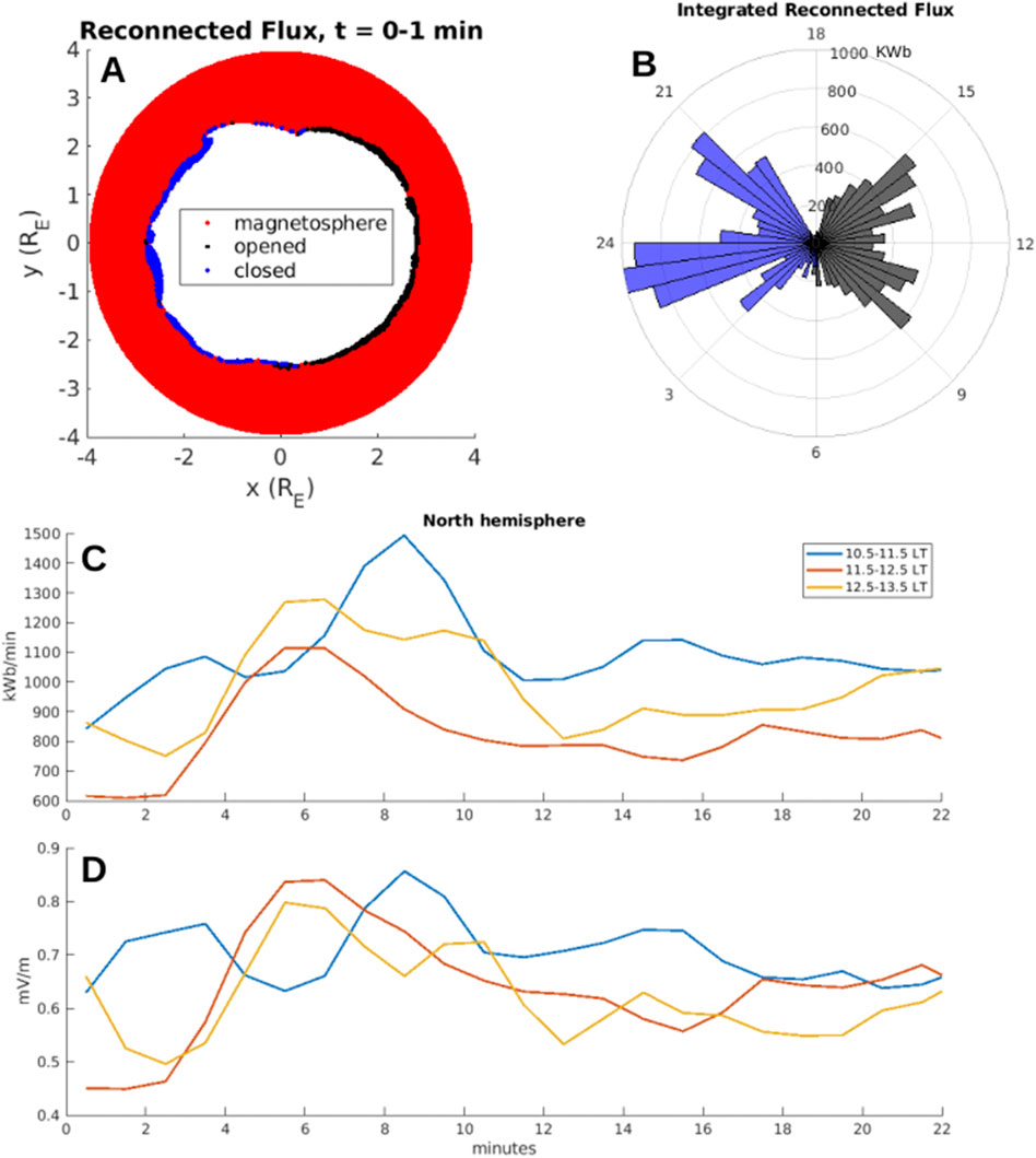
Figure 1. (A) Newly reconnected magnetic flux (blue = newly closed, black = newly opened) in the northern hemisphere. Red and white areas correspond to locations where the magnetic field did not undergo a reconnection during the 1-min interval (8:00–8:01). (B) Integration of newly reconnected flux in 30-min MLT bins during the same interval. Black corresponds to integrated newly opened flux and blue corresponds to integrated newly closed flux. (C) Time-dependence of integrated newly opened flux for the MLT sectors 10.5–11.5 (blue), 11.5–12.5 (orange), and 12.5–13.5 (yellow). (D) Reconnected flux (KWb/min) is scaled to electric field (mV/m) by $d{y}^{\prime }\sim 3.5$ ${\text{R}}_E$ (see main text for more discussion).

2.2 Cusp ion dispersion

Forward proton test particle tracing is performed in 3D within the GAMERA fields using the Conservative Hamiltonian Integrator for Magnetospheric Particles (CHIMP, Sorathia et al. (2018)). Since the test particle tracing is performed in the MHD post-processing, the GAMERA fields are evolved in time via interpolation between 5 s outputs. Figure 2 demonstrates the global MHD with test particle simulation setup where ions are initialized in the magnetosheath and collected in the cusp. 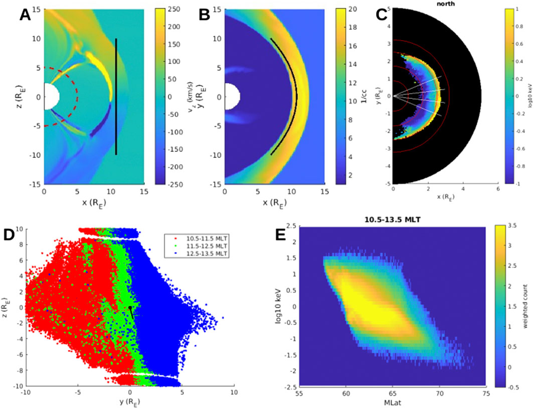Figure 2A shows ${\text{v}}_z$ at $y=0$ and the vertical black line is the $z$-extent (-10 to 10 ${\text{R}}_E$) of the particle injection region at noon magnetic local time (MLT). Figure 2B is an equatorial slice of density and the black parabola is the shape of the particle injection region in the $x-y$ plane (the $z$-extent is -10 to 10 ${\text{R}}_E$ at all MLT). The particle injection region is designed to initialize particles close to the magnetopause without crossing it, especially near the equator where the x-line is mostly located for southward dominant IMF. The collection altitude is 5 ${\text{R}}_E$ (red dashed circle, Figure 2A), which is below the altitude where the dipole field no longer dominates. Spacecraft missions such as TRACERS and DMSP, which observe cusp ion dispersions, fly at much lower altitudes, so in order to make direct comparison it will be necessary to map simulated ion dispersions down magnetic field lines. However, the methodology to calculate reconnection rate from ion dispersions (see below) can be applied at any altitude, so for this theoretical study there is no attempt to map ion dispersions to ionospheric altitudes. To establish a constant flux into the cusp for particles with a range of energies, ions are continuously streamed into the simulation from 8:00–8:10. The fastest particles reach 5 ${\text{R}}_E$ in $\sim 2.5$ minutes and thus ion dispersions are constructed from 8:08–8:12 (allowing time for low energy particles to reach the collection height and also avoiding the start and end of particle streaming).

Figure 2

Figure 2. (A) ${\text{v}}_z$ at y = 0 in the global MHD simulation (t = 8:00). The black line shows the $z$-extent of the particle injection region at noon MLT and the dashed red circle shows the altitude where particles are collected. (B) Density at $z$ = 0 (the magnetopause is the innermost strong density gradient, the white circle is the MHD inner boundary). The black parabola shows the shape of the particle injection region in the $x-y$ plane. (C) North hemisphere at 5 ${\text{R}}_E$ (black). Colormap shows the average energy (on a logarithmic scale) of particles collected in the cusp. White lines bound the 10.5–11.5, 11.5–12.5, and 12.5–13.5 MLT sectors and red MLat circles are 50, 60, 70, and 80°. (D) Initial location (in the $y-z$ plane) of particles colored by MLT of collection in the cusp (red 10.5–11.5, green 11.5–12.5, blue 12.5–13.5). The solid black line indicates IMF orientation. (E) MLat-Energy spectrogram of particles collected in the northern cusp integrated over the local time sector 10.5–13.5 and the entire simulation time.

The initial energy distribution ranges from 10 eV to 100 eV and pitch angles uniformly distributed from 0–180° (Burkholder, 2025). Particles are weighted (based on their initial energies) against a magnetosheath-like distribution of energies represented by a Maxwellian of temperature 100 eV (on the low end of terrestrial magnetosheath temperatures Shen et al. (2022)). The total number of particles initialized was $\sim 1.7$ billion with $\sim 8.8$ million reaching the inner boundary (about 0.5$\%$) over the course of the 15 min simulation (8:00–8:15). Figure 2C bins all particles collected in the northern hemisphere at 5 ${\text{R}}_E$ altitude. The colormap gives the average ion energy (on a logarithmic scale) that was collected in each bin, which has a clear trend of higher energy particles at lower MLat (MLat in this study is defined as the polar angle at 5 ${\text{R}}_E$ altitude, different than the typical definition which would be mapped along magnetic field lines to Earth’s surface) and lower energy particles at higher MLat (red circles show MLat = 80, 70, 60, 50°). To construct simulated cusp ion dispersions, virtual satellites are launched at 5 ${\text{R}}_E$ altitude moving from 58.9 to 67.2° MLat in 1-min. At each latitudinal step, the spacecraft collects particles in a bin size of 0.5° MLat $\times$ 1 h MLT. The three MLT sectors 10.5–11.5, 11.5–12.5, and 12.5–13.5 are bounded by white lines in Figure 2C.

Figure 2D shows the initial location of those ions collected at 5 ${\text{R}}_E$ with color corresponding to MLT where they were collected (the black line indicates IMF orientation). Only particles that hit the inner boundary from 10.5–13.5 MLT (10.5–11.5 red, 11.5–12.5 green, 12.5–13.5 blue) are shown. The vertical striping pattern indicates that the initial MLT of particles roughly corresponds to MLT in the cusp where they are collected. This is an important aspect of these simulations, because when simulating real events, the location where particles hit the inner boundary should preferably be concentrated to the location of real spacecraft observations (to achieve sufficient particle statistics at minimum computational cost). Figure 2D also shows a gap around $z\sim \pm 9$ ${\text{R}}_E$ corresponding to a relatively small population of particles which do not make it into the cusp. Apparently, those particles initialized too close to the bow shock are not able to access the cusp regardless of initial energy or pitch angle (within the limits of the initial distribution in this study). Figure 2E is an energy-latitude spectrogram of all particles that were collected at 5 ${\text{R}}_E$ in the 10.5–13.5 MLT sector (integrated over the entire simulation time). The typical dispersion signature (higher energy particles at lower MLat, lower energy particles at higher MLat) is clearly evident in the time-integrated representation. Notice, such a visualization does not represent an observable cusp ion dispersion (because it is time and spatially integrated), but synthetic satellites that collect particles in a finite-sized moving bin can construct representative cusp ion dispersions for which the reconnection rate can be calculated.

From Lockwood and Smith (1992), the magnetopause reconnection rate $E_y^{\prime }$ can be calculated

$E_y^{\prime }=\left(dy/d{y}^{\prime }\right)E_y$

where $d{y}^{\prime }$ is the length of the X-line segment which maps down the magnetic field to the length $dy$ of the merging gap in the ionosphere, and $E_y$ is the electric field along the merging gap:

$E_y=\left(B_s{V}_s\cos \alpha \right){\left(1+\left(d^{\prime }/2\right){\left(m/2\right)}^{1/2}{\mathcal{E}}_{ic}^{-3/2}d{\mathcal{E}}_{ic}/d{t}_s\right)}^{-1}.(1)$

$B_s$ is the magnetic field strength at the spacecraft, $V_s$ is spacecraft velocity, $\alpha$ is the angle between $V_s$ and the direction of flux tube convection, $d^{\prime }$ is the distance from the x-line to the ionosphere (along newly reconnected field lines) lengthened to account for ${\text{E}}_{\Vert }$, and $m$ is the ion mass. The quantity extracted from the cusp ion dispersion is ${\mathcal{E}}_{ic}$, which is the low energy cutoff. ${\mathcal{E}}_{ic}$ is the minimum ion energy on a given field line that is precipitating at a given latitude. The definition from Lockwood and Smith (1992) is adopted, where ${\mathcal{E}}_{ic}$ is the energy at which the flux is some fraction of the peak flux. The exact value of the fraction is varied in this study. The time increment $d{t}_s$ is the time resolution of the (virtual) ion instrument. The derivative $d{\mathcal{E}}_{ic}/d{t}_s$ is calculated from a three-point central difference of ${\mathcal{E}}_{ic}$ where the energy bins of the virtual instrument are uniformly separated in log space. Two different time and energy resolutions are used (described below) to compare calculated reconnection rates for a virtual “TRACERS” and “DMSP.”

Global simulations are necessary to provide the length scales and magnetic field strengths in Equation 1 because these global variables are inaccessible to a single spacecraft. The quantity $dy/d{y}^{\prime }=0.23$ for $dy=0.8$ ${\text{R}}_E$ and $d{y}^{\prime }$ = 3.5 ${\text{R}}_E$. The ratio $dy/d{y}^{\prime }$ can also be calculated using the flux tube expansion factor $dy/d{y}^{\prime }\sim \sqrt{B_{mp}/B_s}$ with ${\text{B}}_{mp}$ the magnetic field strength just inside the magnetopause (Lockwood and Smith, 1992; da Silva et al., 2025). At 5 ${\text{R}}_E$, ${\text{B}}_s\sim 400$ nT where the virtual spacecraft trajectory first encounters ions in the cusp, and just inside the magnetopause, ${\text{B}}_{mp}\sim 60$ nT, which gives $dy/d{y}^{\prime }\sim 0.39$. A constant value $dy/d{y}^{\prime }=0.3$ is used as an estimate. The quantity $d^{\prime }$ is a virtual distance along magnetic field lines that is lengthened to account for $E_{\Vert }$ as ions move into the cusp. Since the test particles do not experience any $E_{\Vert }$, $d^{\prime }$ in this study is replaced with $d$, the distance along magnetic field lines from the x-line to the spacecraft. From 8:00–8:15, in the 10.5–11.5 MLT sector $d\sim 10.8-13.3$ ${\text{R}}_E$, in the 11.5–12.5 MLT sector $d\sim 12.2-13.5$ ${\text{R}}_E$, and in the 12.5–13.5 MLT sector $d\sim 10.5-12.9$ ${\text{R}}_E$. The values $d=12.05$, $d=12.85$, and $d=11.7$ ${\text{R}}_E$ are taken as fixed estimates for the local time sectors 10.5–11.5, 11.5–12.5, and 12.5–13.5, respectively. The quantity $\alpha$ is taken to be zero which is a good approximation near noon local time under southward dominant IMF and for virtual spacecraft at constant magnetic longitude. $V_s$ is chosen such that the spacecraft crosses the ion dispersion at 5 ${\text{R}}_E$ altitude in 1 min, similar to DMSP events (see, e.g., da Silva et al. (2022) Figure 1).

Note, the global MHD with test particle approach neglects some physical processes which could modify the simulated ion dispersions (see Drake et al. (2009) for comparison of ion acceleration downstream of the x-line in test particle versus fully kinetic simulations). Specifically, the test particle approach does not include self-consistent feedback between the particles and fields (which can be important for phenomena like solar flares where the number of accelerated particles is sufficiently large, see Zharkova et al. (2011)). Additionally, MHD does not realistically capture the reconnection diffusion region, especially the structure of magnetic field parallel electric fields $(E_{\Vert })$ that efficiently accelerate particles. In fact, CHIMP removes $E_{\Vert }$ to avoid anomalous particle heating (see Sorathia et al. (2018) Appendix A1 for discussion). Despite these limitations of the model, all that is needed to have dispersed particles in the low-altitude cusp is a population of particles with a range of energies entering the cusp from the magnetosheath. The dispersion of particles is a result of large scale convection of the magnetic field, which is well captured by the MHD approximation. The exact mechanism or magnitude of particle acceleration at the x-line does not affect the calculation of the reconnection rate.

3 Results

3.1 Reconnection rate from change of magnetic flux

Figure 1B shows newly opened (black) and newly closed (blue) magnetic flux in 30 min MLT bins (units of kWb represent newly reconnected flux in a 1-min interval). Because the IMF has been steadily southward for 2+ hours, the system has reached a quasi-steady state and there is a symmetry of opening reconnection occurring on the day-side (MLT 6 to 18) and closing reconnection occurring on the night-side (MLT 18–24 and 0–6). At this timestep, the total amount of opened flux is 8,800 kWb and the total amount of closed flux is 9,300 kWb, a difference of less than 3%. Figure 1C shows temporal variation of the simulated reconnection rate in three MLT sectors 10.5–11.5, 11.5–12.5, and 12.5–13.5. It is interesting to note that less flux is almost systematically reconnected at noon MLT compared to pre- and post-noon. Notice also, there are relatively large variations of $\sim 30-40\%$ on a time scale of $\sim 5$ minutes.

Ouellette et al. (2010) calculated the reconnection rate using the Lyon-Fedder-Mobarry (LFM) simulation, the predecessor to GAMERA, and found for purely southward IMF the reconnection rate spanning the entire day-side x-line was $\sim 220$ kV. Figure 1C shows a typical value of the reconnection rate in a 1-h MLT sector is $\sim 1000$ kWb/min. Multiplying by 12 to cover the entire day-side and converting to kilovolts gives 200 kV, consistent with Ouellette et al. (2010). The reconnection rate in units of mV/m is obtained by scaling the newly reconnected flux rate (kWb/min) with $d{y}^{\prime }$, the length of the reconnection x-line on the day-side magnetopause. For the solar wind and IMF conditions in this study, a 1-h MLT sector of the cusp at 5 ${\text{R}}_E$ altitude maps to $d{y}^{\prime }\sim$3.5 ${\text{R}}_E$ on the magnetopause, with some variation due to motions of the x-line. Figure 1D shows reconnection rate (units of mV/m) scaled by $d{y}^{\prime }$ (including time-dependence). After scaling, the noon MLT reconnection rate in units of mV/m is not noticeably different than the pre- and post-noon sectors. The largest variations are about 0.2 mV/m compared to the average value $\sim 0.65$ mV/m, similar to $\sim 30\%$ variations from Figure 1C.

Figure 1 demonstrates that, despite the IMF and solar wind being steady (and having been that way for 2+ hours), there are up to 0.2 mV/m $(\sim 30\%)$ variations of the reconnection rate on a 5–10 min timescale. Figure 3 shows that these variations are associated with spontaneous generation of flux ropes on the magnetopause. The three columns from left to right represent the 10.5–11.5, 11.5–12.5, and 12.5–13.5 MLT sectors, respectively. Each colormap is a 1-h stack plot (1-min time resolution) of thermal pressure on the day-side magnetopause (from z = −5 to 5 ${\text{R}}_E$) in a constant MLT slice (see MLT in each panel title), with the magnetopause shape determined at each time step based on the gradient of thermal pressure. Flux ropes appear as pressure enhancements (Burkholder et al., 2023b) that move up or down in the stack plot, corresponding to motion towards the northern or southern cusp. The strongest flux rope signatures are highlighted with red arrows, and these are generally associated with large $>0.1$ mV/m variations of the reconnection rate (see reconnection rates in Figures 3p–r). It has been suggested that plasmoid formation accelerates reconnection by breaking up the current sheet into segments with smaller effective lengths than the initial current sheet, or through the onset of anomalous-resistivity (Shibata and Tanuma, 2001). Although, exactly how the flux rope formation process influences the reconnection rate depends on the details of the plasmoid evolution in the nonlinear regime where there is a competition between three processes: growth and saturation of plasmoids, plasmoid coalescence, and expulsion of plasmoids along the current sheet by the reconnection outflows (Loureiro et al., 2007). Despite this complicated interaction, Figure 3 shows that when there are no flux rope signatures on the magnetopause, the simulated reconnection rate is steady to within typical noise-level $\sim 0.1$ mV/m variations, whereas the formation and evolution of a flux rope can cause the reconnection rate to vary by up to 0.2 mV/m. How this minimum reconnection rate fluctuation scales with different parameters is an important question left for future work.

Figure 3

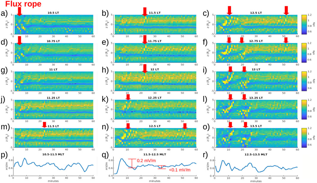
Figure 3. (a–o) Simulated thermal pressure on the day-side magnetopause (from z = −5 to 5 ${\text{R}}_E$) in constant MLT slices (see titles for MLT values). Columns cover the 10.5–11.5, 11.5–12.5, and 12.5–13.5 MLT sectors with 5 slices per hour of MLT. Red arrows highlight magnetopause flux ropes (pressure enhancements moving north or south). (p–r) Opening reconnection rate for the 10.5–11.5, 11.5–12.5, and 12.5–13.5 MLT sectors, respectively. Large variations $\sim 0.2$ mV/m are associated with flux ropes, while the background “noise” level is $\sim 0.1$ mV/m.

3.2 Reconnection rate from cusp ion dispersion

Examples of reconnection rates calculated from simulated cusp ion dispersions are shown in Figure 4. The virtual spacecraft was launched at 8:08:20 moving from low to high MLat in the northern hemisphere. The MLat resolution is 0.25° (this is half the bin size of 0.5° so particles are collected in more than 1 pixel per latitudinal step), corresponding to a time resolution of 1.8 s (the time resolution of the TRACERS ion instrument is $\sim 0.3$ seconds, but this study is limited by the 1-s output resolution of the test particle simulation). The energy resolution of the virtual satellite (13.8 logarithmically space bins per order of magnitude energy) corresponds to the TRACERS ion instrument (Fuselier et al., 2025). Figures 4a–c are simulated cusp ion dispersions in three different local time sectors ((a) 10.5–11.5, (b) 11.5–12.5, and (c) 12.5–13.5). Dispersions (a) and (c) are typical southward IMF examples with 1 keV ions at $\sim 61$ degrees and 0.1 keV ions at $\sim 65-66$ degrees (dispersion (b) is similar but has an overlapping dispersion). ${\mathcal{E}}_{ic}$ at each MLat is marked by a colored dot. The different colors correspond to different fractions of the maximum flux (red 20%, green 60%, black 100%, hereafter referred to as the “${\mathcal{E}}_{ic}$ fraction”). In Figure 4a, the higher ${\mathcal{E}}_{ic}$ fractions provide a better representation of the slope of the main dispersion signature. Although, other than the small bump around 62° MLat, the slopes for black, green, and red generally agree. This suggests that for real events it may be beneficial to have the ${\mathcal{E}}_{ic}$ fraction as a free parameter rather than to set a strict value, in order to minimize or remove the effect of secondary structures in the dispersion signature. Figure 4b shows another example where a higher fraction produces a different profile of ${\mathcal{E}}_{ic}$. Similar overlapping dispersions are formed even for a much smaller sized virtual spacecraft bin. The origin of these in the simulation is discussed in Burkholder et al. (2024b). For this study, overlapping dispersions are not treated differently than single dispersions, leading to a jump of ${\mathcal{E}}_{ic}$ in the region of overlap. To account for this and other imperfections in the dispersion signatures, if $d{\mathcal{E}}_{ic}/dt$ is zero or positive, no value of $E_y^{\prime }$ is calculated. In Figures 4d–f, $E_y^{\prime }$ (left side blue axis) is calculated for each ion dispersion as a function of MLat. The different colors correspond to different ${\mathcal{E}}_{ic}$ fractions. There is no systematic trend for varying the ${\mathcal{E}}_{ic}$ fraction, which supports the idea that this should be left as a free parameter to choose whatever best fits the dispersion. The magnitudes $\sim 0.5-1.0$ mV/m are similar to Figure 1D, yet there are also relatively large $\sim 1$ mV/m variations and a few outliers. Clearly, in some instances ${\mathcal{E}}_{ic}$ has not been perfectly determined ($E_y^{\prime }\sim -2.5$ mV/m in Figure 4e is associated with ${\mathcal{E}}_{ic}$ jumping from the upper to lower branch of a double dispersion), but there is also the statistical nature of the test particle simulation, which is similar to real data in that there can be a significant amount of noise. The right-side orange axes of Figures 4d–f show $E_y$ for the ion dispersions ($E_y^{\prime }$ before it has been mapped to the x-line) compared to the dashed orange, which is the magnitude of $\mathbf{E}=-\mathbf{v}\times \mathbf{B}$ along the path of the spacecraft at 8:08. The magnitude of the local simulation electric field in the region of the ion dispersion is $\sim 3-7$ mV/m, in the same range as the ion dispersions.

Figure 4

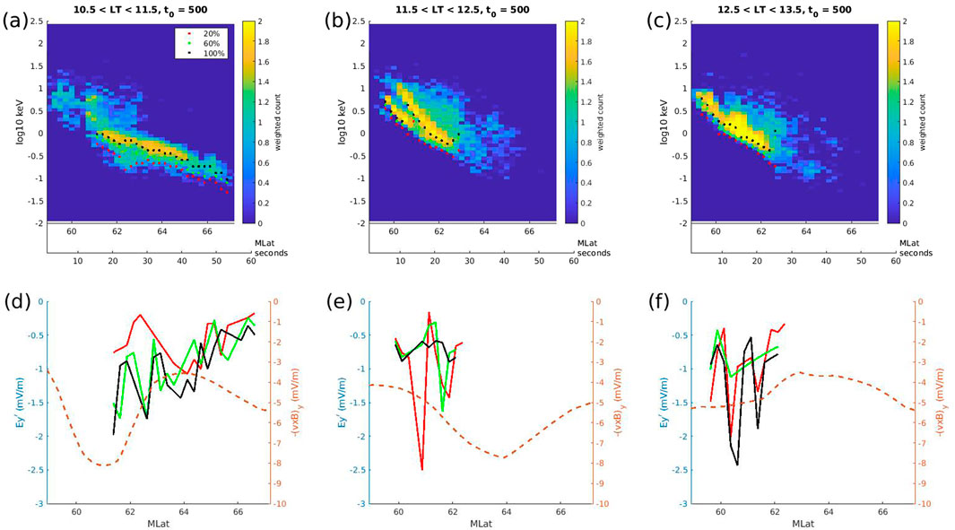
Figure 4. Simulated cusp ion dispersions collected by the virtual satellite (with TRACERS-like energy and time resolution) in three different local time bins (a) 10.5–11.5, (b) 11.5–12.5, (c) 12.5–13.5 at ${\text{t}}_0$ = 8:08:20. Different colored dots show ${\mathcal{E}}_{ic}$ at each MLat for different values of the ${\mathcal{E}}_{ic}$ fraction (defined in main text). (d–f) $E_y^{\prime }$ (left side blue axis) for the corresponding ion dispersion calculated wherever $d{\mathcal{E}}_{ic}/dt<0$. Colors corrsepond to different ${\mathcal{E}}_{ic}$ fractions. The right side orange axis corresponds to $E_y$, the electric field at the spacecraft location estimated from the ion dispersion. The orange dashed line shows the magnitude of $\mathbf{E}=-\mathbf{v}\times \mathbf{B}$ along the spacecraft trajectory in the MHD simulation at 8:08.

Figure 5 shows a sequence of ion dispersions constructed using a TRACERS-like (d-f) and DMSP-like (a-c,g-i) virtual ion instrument (for simplicity the ${\mathcal{E}}_{ic}$ fraction is set at 60%). The DMSP-like instrument has half the time resolution of the TRACERS-like instrument (the real TRACERS has three times higher time resolution) and the energy resolution is the same as the DMSP ion instrument (8 logarithmically space bins per order of magnitude energy, Redmon et al. (2017)). Figures 5A–C show the local time sectors 10.5–11.5, 11.5–12.5, and 12.5–13.5, respectively, at the same time as Figure 4 (${\text{t}}_0$ = 8:08:20). Similarly, Figures 5d–i are virtual TRACERS and DMSP ion dispersions at ${\text{t}}_0$ = 8:11:40. A key difference to note between the TRACERS-like and DMSP-like instruments is the ability to resolve overlapping dispersions (Figures 4b, 5b) and other sub-structures with higher time and energy resolution.

Figure 5

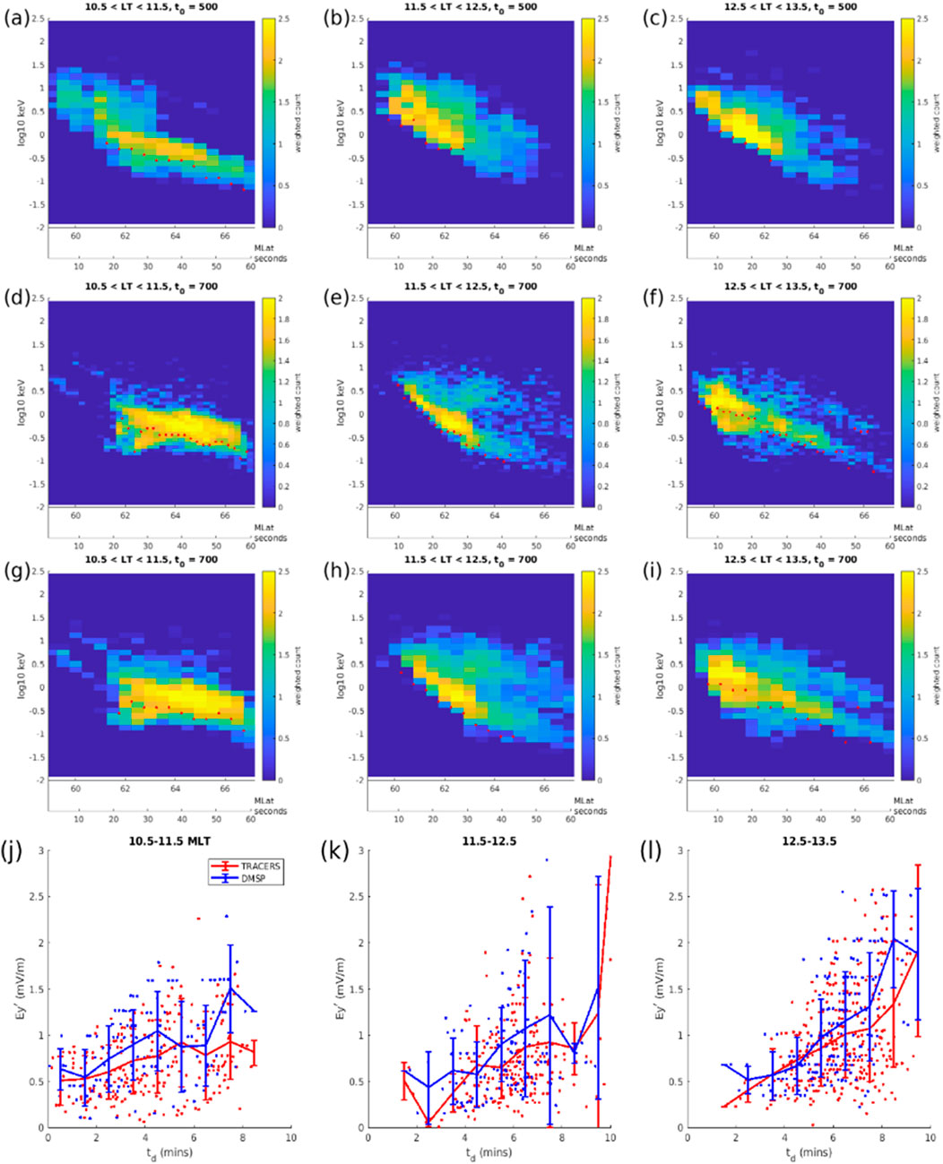
Figure 5. (a–i) Simulated cusp ion dispersions in three MLT sectors 10.5–11.5, 11.5–12.5 and 12.5–13.5 (columns). Red dots show ${\mathcal{E}}_{ic}$ at each MLat using a 60% ${\mathcal{E}}_{ic}$ fraction. For the same time as Figure 4 (${\text{t}}_0$ = 8:08:20), (a–c) shows ion dispersions constructed with a DMSP-like ion instrument. (d–f) and (g–i) show simulated ion dispersions at ${\text{t}}_0$ = 8:11:40 from the TRACERS-like and DMSP-like instruments, respectively. (j–l) Time-dependence of $E_y^{\prime }$ (red - TRACERS, blue - DMSP) with each value plotted as a function of $t_d$ estimating when a particle with field aligned energy ${\mathcal{E}}_{ic}$ was present at the x-line (see main text for more discussion). Solid curves represent average $E_y^{\prime }$ in 30-s bins and the errors bars are 1-standard deviation within each bin.

An ion dispersion is constructed with ${\text{t}}_0$ every 10 s in the interval 8:08:20–8:12:40 (21 total dispersions). An important consideration for the reconnection rate calculation is that particles collected in the cusp crossed the magnetopause at different times. For instance, a 0.1 keV field-aligned proton takes $\sim$9 min to traverse $d=12$ ${\text{R}}_E$, while at 1 keV the travel time is $\sim$3 min (these estimates neglect the mirror force, so the time delay is actually longer, but since particles are collected at 5 ${\text{R}}_E$ in the simulation, the effect is less compared to particles traveling to the ionosphere). To estimate what time at the x-line the reconnection rates correspond to, a time delay is calculated for each reconnection rate to estimate when a particle of energy ${\mathcal{E}}_{ic}$ was at the x-line. The time delay represents the amount of time it takes a field-aligned particle with energy ${\mathcal{E}}_{ic}$ to travel a distance $d$. The time at the x-line $t_d$ is then estimated:

$t_d=t_{\mathit{obs}}-d/v_{\mathit{Eic}},(2)$

where $t_{\mathit{obs}}$ is the observation time of ${\mathcal{E}}_{ic}$ at a particular MLat and $v_{\mathit{Eic}}$ is the velocity of a field-aligned proton with energy ${\mathcal{E}}_{ic}$. This estimate represents a zeroth order approximation as it neglects a number of factors including the mirror force and time variations of $d$. It also does not account for the possibility that $d$ depends on energy, which would be the case if all of the highest energy particles collected in the cusp crossed the magnetopause closest to the x-line and lower energy particles entered after the field line had convected away from the x-line. Figures 5j–l show the reconnection rates calculated using virtual TRACERS-like (red) and DMSP-like (blue) ion instruments (with $t_d$ on the $x$-axis). There are a few hundred points because each ion dispersion produces $\sim 10$ values of the reconnection rate and 21 ion dispersions were constructed in each MLT sector. The solid lines represent the average value of reconnection rate in 0.5 min intervals, with the error bars corresponding to 1-standard deviation in the interval. There is a slight preference for DMSP to be systematically larger, but mostly both instruments agree on the reconnection rate in all three local time sectors (10.5–11.5 Figure 5j, 11.5–12.5 Figure 5k, 12.5–13 Figure 5l). The difference of DMSP- versus TRACERS-like instruments is generally $\sim 0.1-0.2$ mV/m or less, with only a few instances where the error bars are not overlapping. The difference is essentially the same as the level of variation introduced by flux rope formation and evolution. While the DMSP- and TRACERS-like approximations are similar for the case of steady southward IMF, higher energy and time resolution is likely to be key for understanding storm-time and strongly driven reconnection, because for intervals where the reconnection rate is significantly larger, $d{\mathcal{E}}_{ic}/d{t}_s$ will be very shallow. When discretized into bins, the resulting reconnection rate is entirely dependent on whether the slope is sufficiently resolved.

Figures 6a–c show the reconnected flux measure of the reconnection rate for the MLT sectors 10.5–11.5, 11.5–12.5, and 12.5 13.5 (blue, the same as Figure 1d). The colored lines with (1-standard deviation) error bars are the time-delayed ion dispersion calculation of the reconnection rate with a TRACERS-like instrument from 8:08:20–8:12:40 (similar to Figures 5j–l but different colors represent different ${\mathcal{E}}_{ic}$ fractions: red 20%, green 60%, blue 100%). As noted by Lockwood and Smith (1992), the exact value of the ${\mathcal{E}}_{ic}$ fraction does not have a significant effect on the results. The large error bars at later times correspond to the highest energy particles collected in the cusp (since $d/v_{\mathit{Eic}}$ in Equation 2 is smaller for higher ${\mathcal{E}}_{ic}$). In many cases there are relatively few particles in the highest energy bins so ${\mathcal{E}}_{ic}$ and $d{\mathcal{E}}_{ic}/dt$ are not well resolved (see Figure 5) resulting in some spuriously large values of the reconnection rate. Across all three local time sectors, the reconnection rates are remarkably similar, mostly being within a factor of less than 1.5, which is perhaps not coincidentally the same amount of uncertainty in the ratio $dy/d{y}^{\prime }$. Equation 1 only represents the primary rate of steady reconnection, so it is not surprising that the time-dependence does not exactly match for the different measures of the reconnection rate. In fact, by applying a 2D smoothing to the simulated ion spectrograms, the error bars become systematically smaller and the choice of ${\mathcal{E}}_{ic}$ fraction matters even less, since the smoothing out of sub-structures means $d{\mathcal{E}}_{ic}/dt$ is more representative of the primary rate of steady reconnection.

Note, units of the ion energy spectrograms (Figures 4, 5) in this study are particle counts/second, which can be converted to differential energy flux (=count rate/geometric factor) to compare with observations. For a geometric factor with no energy dependence, the calculated reconnection rates would be the same regardless of units. However, the TRACERS ACI has an energy-dependent geometric factor (see (Fuselier et al., 2025) Figure 5), such that the ion energy spectrograms in units of differential energy flux have greater flux (compared to spectrograms in units of weighted count) at lower energy. The result of this is to shift ${\mathcal{E}}_{ic}$ to slightly lower energy at all MLat, which is ultimately the same as choosing a smaller ${\mathcal{E}}_{ic}$ fraction. Indeed, after conversion to differential energy flux, the reconnection rate calculations in Figures 4–6 are almost identical.

Figure 6

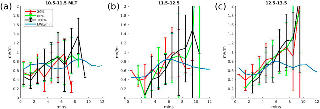
Figure 6. Comparison of the opening reconnection rate (blue) and $E_y^{\prime }$ (from the TRACERS-like virtual instrument) in the MLT sectors 10.5–11.5 (a), 11.5–12.5 (b), and 12.5–13.5 (c). $E_y^{\prime }$ is plotted as a function of $t_d$, an estimate of time at the x-line. Colors represent different values of the ${\mathcal{E}}_{ic}$ fraction (red 20%, green 60%, blue 100%). The solid curves represent the average value of all reconnection rates (calculated from 21 ion dispersions) binned in 30-s intervals, with error bars corresponding to 1-standard deviation within each bin.

4 Discussion and conclusion

The simulated day-side magnetopause reconnection rate based on changes of magnetospheric flux during steady southward IMF has variations of $\sim 0.2$ mV/m superposed onto the mean value of $\sim 0.65$ mV/m. Calculations of the reconnection rate from simulated cusp ion dispersions reproduce this rate to a factor of 2 or less. These reconnection rates are well within the range of values (0.5–2 mV/m) reported by MMS during a quiet time diffusion region encounter with southward IMF. Furthermore, da Silva et al. (2025) calculated reconnection rates on multiple cusp encounters during a moderate geomagnetic storm using DMSP observations. On successive cusp encounters, the reconnection rate was $\sim 1$ mV/m and then $\sim 0.2$ mV/m. Over 7 passes through the cusp the maximum observed reconnection rate was $\sim 2$ mV/m and the minimum was $\sim 0.1$ mV/m, similar to results of this study. The relatively large variations of reconnection rate in the simulation are associated with the formation and evolution of flux ropes. When there is no flux rope activity on the magnetopause, typical variations of the reconnection rate are $\sim 0.1$ mV/m. For future studies of strongly driven reconnection during geomagnetic storms, if reconnection rates are varying by a few mV/m, the capability to calculate reconnection rate to within 1 mV/m will be sufficient to reproduce sufficiently slow (since Equation 1 assumes steady reconnection) time-dependent variations (by examining successive dispersions) of the reconnection rate using the global MHD with test particle approach.

It is important to note that Equation 1 was developed for the simplified scenario of a spacecraft that follows a single convecting field line during an interval of steady day-side reconnection. Since Figure 1 shows that the reconnection rate varies on $\sim 5$ minute timescales, Equation 1 is being applied in a regime where it is not strictly applicable. Although, the level of variation of the simulated reconnection rate is likely to be as steady as the GAMERA simulation will produce, since the solar wind and IMF are idealized. Furthermore, there is some time ambiguity that needs to be understood in order to determine what time at the x-line a single calculation of $E_y^{\prime }$ from a single ion dispersion corresponds to. One way to improve the estimate is to take into account the mirror force in Equation 2, but there remains another aspect that is related to the intrinsically unsteady nature of reconnection in the simulation. Reconnection rate variations up to 0.2 mV/m on a $\sim 5$ minute timescale mean that while a particle is traversing the distance from the x-line to 5 ${\text{R}}_E$ (or $\sim$1 ${\text{R}}_E$ in the case of TRACERS or DMSP) altitude in the cusp, the exhausted magnetic field line convection velocity is not necessarily constant. Since the time scale for ions to travel from the x-line into the cusp is similar to or longer than 5 min (it takes a 1 keV ion $\sim$3 min to traverse $d=12$ ${\text{R}}_E$, and $\sim$9 min at 0.1 keV), the reconnection rate is averaged over some timescale that is related to the time it takes an ion to traverse the distance from the x-line to the low-altitude cusp. Although, this effect may not be significant if the time scale only corresponds to a short interval when the exhausted field line is still close to the x-line. Anyway, it is important to note that the two measures of reconnection rate in this study are fundamentally different. The magnetic topology changes are averaged over a 1-min interval while the ion dispersions have a different amount of averaging for different energies. Dispersed electrons in the cusp, which are a science target for both TRACERS and the Observing Cusp High-Altitude Reconnection Electrodynamics (OCHRE) student rocket mission (Powers et al., 2025), could provide a near instantaneous measure of the reconnection rate, since electrons travel 10 ${\text{R}}_E$ in 10 s or less at energies of 0.1 keV and greater.

Not only are simulations necessary to determine the relevant length scales for Equation 1, but they provide the means to understand particle trajectories and magnetic reconnection dynamics associated with cusp ion dispersions. This would only otherwise be possible observationally during fortuitous spacecraft alignments. For the steady southward IMF simulation in this study, the parameters $d$ and $dy/d{y}^{\prime }$ are essentially constant, but for real events they can vary on minute timescales (especially during strongly driven geomagnetic storm conditions). Time dependent values for $d$ and $dy/d{y}^{\prime }$ can be calculated in global MHD simulations of real events (notice it is possible to calculate $d$ but not $d^{\prime }$). In addition, for real events it will be most important to construct dispersion signatures in a certain part of the cusp where TRACERS or some other spacecraft flew through it (as opposed to the entire cusp), in which case particle initial locations can be chosen so that as many as possible hit the simulation inner boundary on magnetic field lines connected to TRACERS (particle back tracing is also an option to localize particles). Notice that with the current simulation setup there is a sizable gap between the inner boundary of the global MHD simulation and the altitude of TRACERS. In this study, the gap would be almost 4 ${\text{R}}_E$, a significant fraction $(\sim 1/3)$ of $d$. The collection height can be moved as low as 3 ${\text{R}}_E$ (at the expense of particle statistics) which would reduce the gap to $\sim$ 2 ${\text{R}}_E$, but some method must still be developed to map dispersions to the altitude of TRACERS. Mapping the dispersion signature from the collection height across the gap is non-trivial because field line convection below the inner boundary of the MHD simulation will continue to disperse particles. But the convection velocity in the gap region can be calculated from the $\mathbf{E}\times \mathbf{B}$ velocity (with E defined by the electrostatic potential solved in the ionosphere and mapped along field lines), so future studies can include the mapping to lower altitude in order to compare with TRACERS observations.

Data availability statement

Test particle simulation outputs are archived at Zenodo (Burkholder, 2025). The global MHD simulation is also archived at Zenodo (simulation 4) (Burkholder, 2023).

Author contributions

BB: Conceptualization, Data curation, Formal Analysis, Funding acquisition, Investigation, Methodology, Resources, Software, Validation, Visualization, Writing – original draft, Writing – review and editing. L-JC: Supervision, Writing – original draft, Writing – review and editing. JD: Writing – original draft, Writing – review and editing. XM: Writing – original draft, Writing – review and editing. DS: Writing – original draft, Writing – review and editing. ID: Writing – original draft, Writing – review and editing. Y-MH: Writing – original draft, Writing – review and editing. NB: Writing – original draft, Writing – review and editing. KS: Writing – original draft, Writing – review and editing.

Funding

The author(s) declare that financial support was received for the research and/or publication of this article. Funding for this work is provided by a NASA Magnetospheric Multiscale (MMS) Early Career Award 80NSSC25K7352.

Acknowledgments

Acknowledgements

We acknowledge use of the Texas Advanced Computing Center (TACC) at The University of Texas at Austin for providing HPC resources that have contributed to the research results reported within this paper http://www.tacc.utexas.edu. GAMERA-REMIX-CHIMP is part of the Multiscale Atmosphere-Geospace Environment (MAGE) model developed by the NASA DRIVE Science Center for Geospace Storms (https://cgs.jhuapl.edu/MAGE/). We thank the team of the Center for Geospace Storms for providing the GAMERA-REMIX-CHIMP model.

Conflict of interest

The authors declare that the research was conducted in the absence of any commercial or financial relationships that could be construed as a potential conflict of interest.

Generative AI statement

The author(s) declare that no Generative AI was used in the creation of this manuscript.

Any alternative text (alt text) provided alongside figures in this article has been generated by Frontiers with the support of artificial intelligence and reasonable efforts have been made to ensure accuracy, including review by the authors wherever possible. If you identify any issues, please contact us.

Publisher’s note

All claims expressed in this article are solely those of the authors and do not necessarily represent those of their affiliated organizations, or those of the publisher, the editors and the reviewers. Any product that may be evaluated in this article, or claim that may be made by its manufacturer, is not guaranteed or endorsed by the publisher.

References

Birn, J., Drake, J. F., Shay, M. A., Rogers, B. N., Denton, R. E., Hesse, M., et al. (2001). Geospace environmental modeling (gem) magnetic reconnection challenge. J. Geophys. Res. Space Phys. 106, 3715–3719. doi:10.1029/1999JA900449

CrossRef Full Text | Google Scholar

Birn, J., Galsgaard, K., Hesse, M., Hoshino, M., Huba, J., Lapenta, G., et al. (2005). Forced magnetic reconnection. Geophys. Res. Lett. 32. doi:10.1029/2004GL022058

CrossRef Full Text | Google Scholar

Burch, J. L., Webster, J. M., Hesse, M., Genestreti, K. J., Denton, R. E., Phan, T. D., et al. (2020). Electron inflow velocities and reconnection rates at earth’s magnetopause and magnetosheath. Geophys. Res. Lett. 47, e2020GL089082. doi:10.1029/2020GL089082

CrossRef Full Text | Google Scholar

Burkholder, B. (2023b). “Gamera global mhd: ideal simulations,” Zenodo, Published February 27, 2023, Version v1. doi:10.5281/zenodo.7675548

CrossRef Full Text | Google Scholar

Burkholder, B. (2025). “Ion test particle simulations,” Zenodo, Published August 21, 2025, Version v1. doi:10.5281/zenodo.16920753

CrossRef Full Text | Google Scholar

Burkholder, B. L., Chen, L.-J., Sorathia, K., Sciola, A., Merkin, S., Trattner, K. J., et al. (2023a). The complexity of the day-side x-line during southward interplanetary magnetic field. Front. Astronomy Space Sci. 10, 1175697. doi:10.3389/fspas.2023.1175697

CrossRef Full Text | Google Scholar

Burkholder, B. L., Chen, L.-J., Sarantos, M., Gershman, D. J., Argall, M. R., Chen, Y., et al. (2024a). Global magnetic reconnection during sustained sub-alfvénic solar wind driving. Geophys. Res. Lett. 51, e2024GL108311. doi:10.1029/2024GL108311

CrossRef Full Text | Google Scholar

Burkholder, B. L., Girma, Y., Porter, A., Chen, L.-J., Dorelli, J., Ma, X., et al. (2024b). Overlapping cusp ion dispersions formed by flux ropes on the day-side magnetopause. Front. Astronomy Space Sci. 11, 1430966–1432024. doi:10.3389/fspas.2024.1430966

CrossRef Full Text | Google Scholar

Chandler, M. O., Avanov, L. A., Craven, P. D., Mozer, F. S., and Moore, T. E. (2008). Observations of the ion signatures of double merging and the formation of newly closed field lines. Geophys. Res. Lett. 35. doi:10.1029/2008GL033910

CrossRef Full Text | Google Scholar

Connor, H. K., Raeder, J., Sibeck, D. G., and Trattner, K. J. (2015). Relation between cusp ion structures and dayside reconnection for four imf clock angles: Openggcm-ltpt results. J. Geophys. Res. Space Phys. 120, 4890–4906. doi:10.1002/2015JA021156

CrossRef Full Text | Google Scholar

da Silva, D., Chen, L. J., Fuselier, S., Wang, S., Elkington, S., Dorelli, J., et al. (2022). Automatic identification and new observations of ion energy dispersion events in the cusp ionosphere. J. Geophys. Res. Space Phys. 127, e2021JA029637. doi:10.1029/2021JA029637

CrossRef Full Text | Google Scholar

da Silva, D. E., Chen, L. J., Fuselier, S. A., Petrinec, S. M., Trattner, K. J., Cucho-Padin, G., et al. (2024). Statistical analysis of overlapping double ion energy dispersion events in the northern cusp. Front. Astronomy Space Sci. 10, 1228475. doi:10.3389/fspas.2023.1228475

CrossRef Full Text | Google Scholar

da Silva, D. E., Chen, L. J., Fueslier, S. A., Trattner, K. J., Burkholder, B. L., DesJardin, I. M., et al. (2025). Calculation of the dayside reconnection rate from cusp ion-energy dispersion. Front. Astronomy Space Sci., 12–2025. doi:10.3389/fspas.2025.1607611

CrossRef Full Text | Google Scholar

Drake, J. F., Swisdak, M., Phan, T. D., Cassak, P. A., Shay, M. A., Lepri, S. T., et al. (2009). Ion heating resulting from pickup in magnetic reconnection exhausts. J. Geophys. Res. Space Phys. 114. doi:10.1029/2008JA013701

CrossRef Full Text | Google Scholar

Fuselier, S. A., Freeman, M. A., Kletzing, C. A., Christopherson, S. R., Covello, M. J., De Luna, D., et al. (2025). The analyzer for Cusp ions (ACI) on the TRACERS mission. Space Sci. Rev. 221, 30. doi:10.1007/s11214-025-01154-w

PubMed Abstract | CrossRef Full Text | Google Scholar

Karimabadi, H., Roytershteyn, V., Daughton, W., and Liu, Y.-H. (2013). Recent evolution in the theory of magnetic reconnection and its connection with turbulence. Space Sci. Rev. 178, 307–323. doi:10.1007/s11214-013-0021-7

CrossRef Full Text | Google Scholar

Lockwood, M. (1995). Overlapping cusp ion injections: an explanation invoking magnetopause reconnection. Geophys. Res. Lett. 22, 1141–1144. doi:10.1029/95GL00811

CrossRef Full Text | Google Scholar

Lockwood, M., and Smith, M. F. (1992). The variation of reconnection rate at the dayside magnetopause and cusp ion precipitation. J. Geophys. Res. Space Phys. 97, 14841–14847. doi:10.1029/92JA01261

CrossRef Full Text | Google Scholar

Loureiro, N. F., Schekochihin, A. A., and Cowley, S. C. (2007). Instability of current sheets and formation of plasmoid chains. Phys. Plasmas 14, 100703. doi:10.1063/1.2783986

CrossRef Full Text | Google Scholar

Merkin, V. G., and Lyon, J. G. (2010). Effects of the low-latitude ionospheric boundary condition on the global magnetosphere. J. Geophys. Res. Space Phys. 115. doi:10.1029/2010JA015461

CrossRef Full Text | Google Scholar

Merkin, V. G., Lyon, J. G., and Claudepierre, S. G. (2013). Kelvin-Helmholtz instability of the magnetospheric boundary in a three-dimensional global MHD simulation during northward IMF conditions. J. Geophys. Res. Space Phys. 118, 5478–5496. doi:10.1002/jgra.50520

CrossRef Full Text | Google Scholar

Miles, D., Kletzing, C., Fuselier, S., Goodrich, K., Bonnell, J., Bounds, S., et al. (2025). The tandem reconnection and cusp electrodynamics reconnaissance satellites (tracers) mission. Space Sci. Rev. 221, 61. doi:10.1007/s11214-025-01184-4

PubMed Abstract | CrossRef Full Text | Google Scholar

Ouellette, J. E., Rogers, B. N., Wiltberger, M., and Lyon, J. G. (2010). Magnetic reconnection at the dayside magnetopause in global lyon-fedder-mobarry simulations. J. Geophys. Res. Space Phys. 115. doi:10.1029/2009JA014886

CrossRef Full Text | Google Scholar

Powers, B. N., Feltman, C. A., Jaynes, A. N., Moore, A. T., Ervin, T., Llera, K., et al. (2025). Observing cusp high-altitude reconnection and electrodynamics: the TRACERS student rocket. Space Sci. Rev. 221, 65. doi:10.1007/s11214-025-01192-4

PubMed Abstract | CrossRef Full Text | Google Scholar

Redmon, R. J., Denig, W. F., Kilcommons, L. M., and Knipp, D. J. (2017). New dmsp database of precipitating auroral electrons and ions. J. Geophys. Res. Space Phys. 122, 9056–9067. doi:10.1002/2016ja023339

PubMed Abstract | CrossRef Full Text | Google Scholar

Shen, C., Ren, N., Qureshi, M. N. S., and Guo, Y. (2022). On the temperatures of planetary magnetosheaths at the subsolar points. J. Geophys. Res. Space Phys. 127, e2022JA030782. doi:10.1029/2022JA030782

CrossRef Full Text | Google Scholar

Shibata, K., and Tanuma, S. (2001). Plasmoid-induced-reconnection and fractal reconnection. Earth, Planets Space 53, 473–482. doi:10.1186/BF03353258

CrossRef Full Text | Google Scholar

Sorathia, K. A., Ukhorskiy, A. Y., Merkin, V. G., Fennell, J. F., and Claudepierre, S. G. (2018). Modeling the depletion and recovery of the outer radiation belt during a geomagnetic storm: combined mhd and test particle simulations. J. Geophys. Res. Space Phys. 123, 5590–5609. doi:10.1029/2018JA025506

CrossRef Full Text | Google Scholar

Sorathia, K. A., Merkin, V. G., Ukhorskiy, A. Y., Allen, R. C., Nykyri, K., and Wing, S. (2019). Solar wind ion entry into the magnetosphere during northward imf. J. Geophys. Res. Space Phys. 124, 5461–5481. doi:10.1029/2019JA026728

PubMed Abstract | CrossRef Full Text | Google Scholar

Sorathia, K. A., Merkin, V. G., Panov, E. V., Zhang, B., Lyon, J. G., Garretson, J., et al. (2020). Ballooning-interchange instability in the near-earth plasma sheet and auroral beads: global magnetospheric modeling at the limit of the mhd approximation. Geophys. Res. Lett. 47, e2020GL088227. doi:10.1029/2020GL088227

PubMed Abstract | CrossRef Full Text | Google Scholar

Trattner, K. J., Coates, A. J., Fazakerley, A. N., Johnstone, A. D., Balsiger, H., Burch, J. L., et al. (1998). Overlapping ion populations in the cusp: polar/timas results. Geophys. Res. Lett. 25, 1621–1624. doi:10.1029/98GL01060

CrossRef Full Text | Google Scholar

Wiltberger, M., Merkin, V., Lyon, J. G., and Ohtani, S. (2015). High-resolution global magnetohydrodynamic simulation of bursty bulk flows. J. Geophys. Res. Space Phys. 120, 4555–4566. doi:10.1002/2015JA021080

CrossRef Full Text | Google Scholar

Woch, J., and Lundin, R. (1992). Magnetosheath plasma precipitation in the polar cusp and its control by the interplanetary magnetic field. J. Geophys. Res. Space Phys. 97, 1421–1430. doi:10.1029/91JA02487

CrossRef Full Text | Google Scholar

Xiong, Y.-T., Han, D.-S., Wang, Z.-w., Shi, R., and Feng, H.-T. (2024). Intermittent lobe reconnection under prolonged northward interplanetary magnetic field condition: insights from cusp spot event observations. Geophys. Res. Lett. 51, e2023GL106387. doi:10.1029/2023GL106387

CrossRef Full Text | Google Scholar

Zhang, B., Sorathia, K. A., Lyon, J. G., Merkin, V. G., Garretson, J. S., and Wiltberger, M. (2019). GAMERA: a three-dimensional finite-volume MHD solver for non-orthogonal curvilinear geometries. Astrophysical J. Suppl. Ser. 244, 20. doi:10.3847/1538-4365/ab3a4c

CrossRef Full Text | Google Scholar

Zharkova, V. V., Arzner, K., Benz, A. O., Browning, P., Dauphin, C., Emslie, A. G., et al. (2011). Recent advances in understanding particle acceleration processes in solar flares. Space Sci. Rev. 159, 357–420. doi:10.1007/s11214-011-9803-y

CrossRef Full Text | Google Scholar