Data Science for Weather Impacts on Crop Yield

1. Introduction

Several studies have shown that the global food production would have to double by 2050 to meet the needs of rising population and diet shifts (Bruinsma, 2009; Tilman et al., 2011; OECD and Food and Agriculture Organization of the United Nations, 2012). However, a prior study found that the current growth rates in yield for the major cereals grown across the globe are insufficient to achieve this target (Ray et al., 2013). According to the Fifth Assessment Report (AR5) of the Intergovernmental Panel on Climate Change (IPCC), surface temperature is projected to rise over the twenty-first century under all assessed emission scenarios with a high degree of likelihood of an increase in the intensity and duration of heat waves and extreme precipitation events in many regions (IPCC, 2013b). This is expected to cause a significant decline in the global crop production (Gourdji et al., 2013; Deryng et al., 2014), thus making the world more food insecure in future. Figures 1A,B are graphics taken from the IPCC AR5 Working Group 2 report on Food Security and Food Production Systems (IPCC, 2013a) which provide a summary of results from several studies on the impact of climate change on yields for four major crops grown in different regions of the world. An overwhelming majority of these studies show a declining trend in yields over the historical period 1960–2013 (shown in Figure 1A), with several of them also projecting major declines in future across different regions of the globe, especially toward the end of the twenty-first century (shown in Figure 1B). The threat to food security from climate change is a critical issue for a number of businesses like food and beverage, retail, agriculture, insurance, biofuels, transportation and weather analytics. With the world population expected to hit 9 Billion by 2050, governments across the globe need to be well-equipped to deal with supply shocks in major cereals.

FIGURE 1

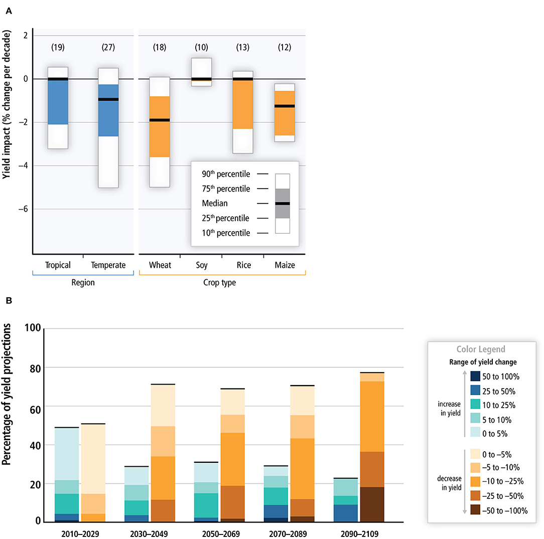
Figure 1. As per the Fifth Assessment Report (AR5) of the IPCC (IPCC, 2013a), changes in temperature and precipitation patterns are expected to cause a significant decline in global crop production. Climate change is also expected to increase the inter-annual variability in yields across different regions. (A) Summary of estimated impacts of historical changes in climate (1960-2013) on yields for four major crops grown in different regions across the globe. Numbers in brackets for each category represent the number of studies. (B) Summary of projected changes in yield over the twenty-first century. This includes projections for different emission scenarios, for temperate and tropical regions, with and without adaptation.

Statistical models and, more recently, tools from machine learning have been used to model crop yield variability using weather indices as inputs. Previous studies have shown the importance of growing season-averaged temperature and precipitation in explaining crop yield variability (Schlenker and Roberts, 2009; Lobell and Burke, 2010; Lobell and Field, 2011; Lobell et al., 2011b; Urban et al., 2012; Osborne and Wheeler, 2013; Moore and Lobell, 2014; Ray et al., 2015). However, extreme weather events from the recent past, like the droughts in Russia in 2010-2011 and in United States (U.S.) in 2012 and their impact on the regional crop production and global commodity markets has clearly made the case to also consider weather extremes in crop yield modeling (Otto et al., 2012). Winter Wheat, for example, has been shown to be particularly susceptible to freezing temperatures during Fall and to heat stress during grain filling and stem elongation (Tack et al., 2015). This vulnerability to extreme temperatures is believed to be the reason behind a decline in wheat yields across Europe (Brisson et al., 2010). As per a different study (Schauberger et al., 2017), each day above 30°C causes a decline in maize and soybean yields by upto 6% under rainfed conditions. Similarly, the interannual variation in rainfall also has a crucial role to play in crop growth. Although a few studies did consider extreme weather indices in their analysis, their scope was either restricted to measuring conditional relationship with yields (Troy et al., 2015) or the extreme event types considered were limited (Lobell and Burke, 2010; Lesk et al., 2016). Non-linear and threshold-type relationships have been shown to exist between yields and weather indices (Schlenker and Roberts, 2009; Lobell et al., 2011a; Troy et al., 2015). However, most of the previous studies have modeled this nonlinearity using regression models with quadratic terms for mean weather indices without appropriate justification. Understanding the exact relationship between weather outcomes and yield is essential given that a prior study reported a significant stagnation and declines in yield for major cereal crops on more than a quarter of global croplands (Ray et al., 2012).

2. Research Questions and Hypotheses

This study addresses the following two research questions:

1. Are extreme weather indices relevant in crop yield modeling?

2. Are nonlinear regression models better at capturing crop yield variability than linear approaches?

Using linear and nonlinear measures for pairwise dependence along with a suite of linear and nonlinear regression models, this study tries to understand the nature of the crop yield-weather relationship with the hypotheses that extreme weather indices have a statistically significant information content and that nonlinear regression models capture yield variability better than linear approaches.

3. Data

In addition to mean weather indices like growing season-averaged maximum and minimum temperature and growing season-averaged precipitation, this study also considered extreme weather indices, as defined by the CCI/CLIVAR/JCOMM Expert team on Climate Change Detection and Indices (ETCCDI) (Karl et al., 1999), as predictors in the regression models. Table 1 provides the list of mean and extreme weather indices along with their definitions. The crop considered for this study was Corn (Maize), a major agricultural input to food production. The U.S. is the largest producer and exporter of this crop with 36% of the world's production (Schlenker and Roberts, 2009). The majority of the U.S. corn production takes place in the midwest region (also known as the “Corn Belt”). The county of Cerro Gordo situated in the state of Iowa in the U.S. midwest was chosen as the area of interest for this study. Yearly values for corn yield (measured in bushels/acre) were collected over a 76-years period starting from 1940 to 2015 from the NASS portal of the USDA (USDA, 2010) for this county. The time series of corn yield over this period, shown in Figure 2, has a strong positive trend due to advancements in farming technology over the years. In order to account for this trend, the year corresponding to the yield was used as one of the predictors in the regression model.

TABLE 1

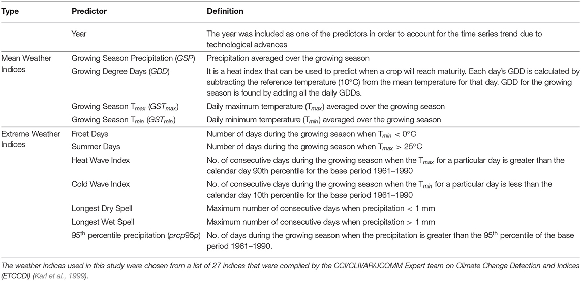
Table 1. Predictor variables used for studying the impact of mean and extreme weather on corn yield.

FIGURE 2

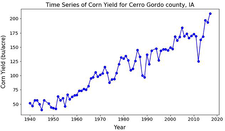
Figure 2. Time series of yearly corn yield (bushels/acre) for Cerro Gordo county over the period 1940–2015. The strong positive trend in the time series can be attributed to advancements in farming technology over the years.

Data for three weather variables: daily maximum temperature (T_max) in °C, daily minimum temperature (T_min) in °C and daily precipitation (Precip) in mm were collected for the period of interest for three weather stations within the county from the Global Historical Climate Network (GHCN) daily database (Menne et al., 2012) using the Climate Data online portal of the National Oceanic and Atmospheric Administration (NOAA) (NOAA, 2018). The county-averaged time series of weather was created by taking an average of the daily data from the three stations, as shown in Figure 3. May 10^th and Oct 20^th were chosen as the start (sowing) and end (harvesting) dates for the growing season and were kept constant over the entire period of interest. Any fluctuations in weather occurring outside the growing period were assumed to have no impact on crop growth. The predictor and response variables were normalized prior to their use by subtracting the mean and dividing by their standard deviation.

FIGURE 3

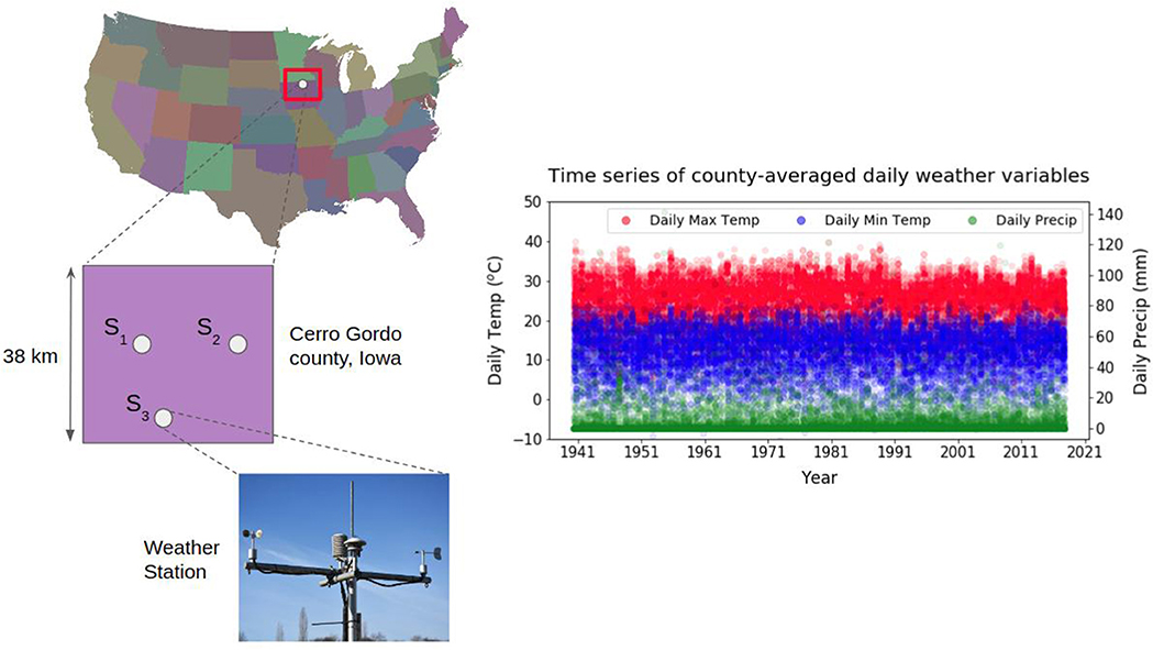
Figure 3. Data for daily maximum and minimum temperature and daily precipitation was collected from three weather stations in Cerro Gordo county, Iowa over the period 1940–2015. Daily county-averaged values for these variables were generated by taking an average over the daily values from the three stations.

4. Methods

4.1. Correlation Between Yield and Weather Indices

Previous studies have used linear correlation measures, such as Pearson correlation coefficient, to estimate the conditional dependence of yield on weather indices. However, multiple studies have shown that this relationship is actually nonlinear and is characterized by the existence of critical thresholds. This study, therefore, uses a correlation coefficient which gives a measure of the overall dependence (linear and nonlinear) between yield and each of the mean and extreme weather indices. This correlation coefficient, namely Mutual Information, is defined in the following section.

4.1.1. Mutual Information

The basic intuition behind information theory is the idea of characterizing the “unpredictability” of a random variable, also known as information entropy. For a random variable X which takes on values in the set χ = {x₁,x₂,…,x_n} with a probability mass function p(x), the entropy H(X) can be formulated as

$\begin{array}{ll}H(X)=-{\displaystyle \sum _{x\epsilon \chi }}p(x)log(p(x))& (1)\end{array}$

The negative sign ensures that entropy is always positive or zero. H(X) can be seen as being approximately equal to how much information we learn from one instance of the random variable X. The information content will be high when the probability is low and vice versa.

Mutual Information (MI) measures how much a random variable tells us about another and is closely related to the concept of entropy. MI for two random variables X and Y, denoted by I(X; Y) can be stated as

$\begin{array}{ll}I(X;Y)=H(X)-H(X|Y)& (2)\end{array}$

where, H(X|Y) is the conditional entropy for X given Y. I(X; Y) measures the average reduction in uncertainty about X that results in learning the value of Y (MacKay, 2003). It is a more general form of correlation coefficient, providing an overall measure of dependence (linear and nonlinear) between two variables (Fraser and Swinney, 1986). The larger the value of MI, the greater is the relationship between the two variables. It is an important statistic when analyzing time series from non-linear systems (Moon et al., 1995). The MI between two random variables X and Y with joint probability mass function p(x, y) and marginal probability density functions (pdfs) p(x) and p(y) is defined as

$\begin{array}{ll}I(X;Y)={\displaystyle \sum _{x\epsilon \chi }}{\displaystyle \sum _{y\epsilon {\rm Y}}}p(x,y)log\frac{p(x,y)}{p(x)p(y)}& (3)\end{array}$

4.1.2. Estimate for Mutual Information

Estimates for MI were obtained using a procedure similar to the one used by Khan et al. (2006). The estimation of MI requires the estimation of joint and marginal pdfs, which were approximated using kernel density estimators (KDE).

For any bivariate dataset (X, Y) of size N, the estimate for MI, $\hat{I}(X;Y)$, is given as

$\begin{array}{ll}\hat{I}(X;Y)=\frac{1}{N}{\displaystyle \sum _{i=1}^N}log\frac{{\hat{p}}_{XY}(x_i;y_i)}{{\hat{p}}_X(x_i){\hat{p}}_Y(y_i)}& (4)\end{array}$

where ${\hat{p}}_{XY}(x_i;y_i)$ is the estimated joint pdf and ${\hat{p}}_X(x_i)$ and ${\hat{p}}_Y(y_i)$ are the estimated marginal pdfs at (x_i, y_i) (Khan et al., 2006).

A gaussian kernel was used for the multivariate kernel density estimator, which is defined as

$\begin{array}{ll}{\hat{p}}_X(x_i)=\frac{1}{N{h}^d}{\displaystyle \sum _{i=1}^N}\frac{1}{\sqrt{{(2\pi )}^d\left|S\right|}}ex{p}^{-\frac{{(x-x_i)}^T{S}^{-1}(x-x_i)}{2h^2}}& (5)\end{array}$

where N is the number of data points; x and x_i are the d-dimensional vectors; S is the covariance matrix on the x_i and h is the kernel bandwidth. For this study, the kernel bandwidth is chosen as $h={\left[\frac{4}{(d+2)}\right]}^{\frac{1}{(d+4)}}{N}^{\frac{-1}{(d+4)}}$. The MI estimates were obtained by first estimating ${\hat{p}}_X$, ${\hat{p}}_Y$, and ${\hat{p}}_{XY}$ using Equation (5) and then using them in Equation (4). The value of MI can vary from 0 to ∞. In order to compare the linear and nonlinear dependence measures, a scaled estimate for MI, denoted as $\hat{\lambda }(X,Y)$ and ranging from 0 to 1 (Joe, 1989; Granger and Lin, 1994), is defined as

$\begin{array}{ll}\hat{\lambda }(X,Y)=\sqrt{1-exp\left[-2\hat{I}(X;Y)\right]}& (6)\end{array}$

Pearson correlation coefficient (ρ), defined in Equation (7), was used to measure linear dependence between two random variables X and Y.

$\begin{array}{ll}\rho =\frac{{\displaystyle {\sum }_{i=1}^N}(x_i-\stackrel{-}{x})(y_i-ȳ)}{\sqrt{{\displaystyle {\sum }_{i=1}^N}{(x_i-\stackrel{-}{x})}^2}\sqrt{{\displaystyle {\sum }_{i=1}^N}{(y_i-ȳ)}^2}}& (7)\end{array}$

In statistics, it is common to estimate the bias and standard error of an estimate. The bias-corrected estimates for $\hat{\lambda }$ and ρ were obtained using jackknife resampling. Resampling was performed using 100 samples of size 0.8 N. The bias for $\hat{\lambda }$ was calculated as $\widehat{bias}$ = $\widehat{\lambda *}$ - $\hat{\lambda }$, where $\hat{\lambda }$ is the original estimate for scaled MI calculated using all N observations and $\widehat{\lambda *}$ is the mean of all jackknife replications. The bias-corrected estimator, $\stackrel{-}{\lambda }$, was defined as $\stackrel{-}{\lambda }$ = $\hat{\lambda }$ - $\widehat{bias}$. The lower and upper bounds of 90% confidence bounds were defined as the 5% and 95% quantiles of the 100 jackknife samples, respectively (Khan et al., 2006). The same method was used to obtain the bias-corrected estimate and error bounds for ρ.

4.2. Linear Regression

Prior to fitting a Multiple Linear Regression (MLR) model with P predictors, Pearson correlation coefficient (ρ) was calculated between each pair of predictor variables to measure pairwise linear dependence, as shown in Figure 4. Many pairs of mean and extreme weather indices were found to have a high absolute value of ρ with one another, implying the presence of a strong positive/negative linear relationship between them. Notable among them are indices like GST_max, GST_min, Summer Days and Heat Wave indices which have a strong positive correlation between them. On the other hand, indices like Frost Days and GST_min have a strong negative linear relationship. The problem of multicollinearity is quite common in weather data and needs to be addressed prior to fitting a linear regression model. Multicollinearity inflates the standard errors of the regression coefficients, making them highly sensitive to minor changes in the model.

FIGURE 4

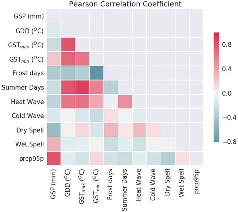
Figure 4. Pearson correlation coefficient was used to measure pairwise linear dependence between predictors. Many pairs of mean and extreme weather indices were found to have high absolute values of correlation, indicating the presence of a strong positive/negative linear relationship. The problem of multicollinearity is quite common in weather data and needs to be addressed before fitting any statistical model.

4.2.1. Principal Component Regression

In order to address the issue of multicollinearity, dimensionality reduction using Principal Component Analysis (PCA) was performed. PCA does feature extraction by taking projections of data along axes of maximum variance (principal components) which are independent of one another (Jolliffe, 1986). Principal Component Regression (PCR) uses these principal components (PCs) as inputs instead of the original correlated features. The appropriate number of PCs to be used as inputs for the MLR model was determined with the help of a cumulative plot of the proportion of variance explained, as shown in Figure 5. By setting a threshold of 95% for the accumulated explained variance, the number of components chosen for the regression was 8. After randomly shuffling the data, about 80% (60 out of 76 samples) was used for fitting the linear model, with the rest used for testing. The resulting PCR model is shown in Equation (8)

$\begin{array}{ll}{y}_i={\beta }_0+{\displaystyle \sum _{j=1}^8}{\beta }_i.P{C}_{ij},& (8)\end{array}$

where β_i are the coefficients.

FIGURE 5

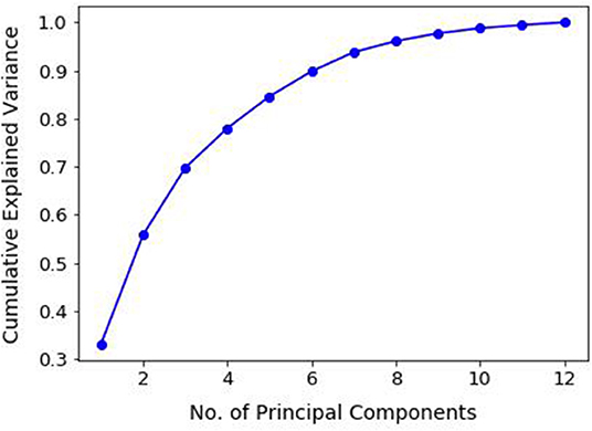
Figure 5. An important step in using Principal Component Regression is the ability to decide how many principal components are needed to describe the data. This can be determined with the help of a plot of cumulative explained variance as a function of the number of principal components. Setting a threshold of 95%, the number of principal components selected for the study was 8.

4.2.2. Ridge Regression

Ridge regression is a technique for creating a multiple regression model for data that are highly correlated (Hoerl and Kennard, 1970). By adding a degree of bias to the model coefficients, ridge regression reduces their variance, thus giving estimates that are more reliable. Equation (9) represents a multiple linear regression model between corn yield and the 12 predictors, with β_j representing the coefficients. In addition to minimizing the deviation from y_i, the objective function for ridge regression, shown in Equation (10), also includes a penalty term that shrinks the coefficient values closer to the “true” population parameters. This penalty term, also referred to as L2 regularization, equals the square of the magnitude of coefficients. The tuning parameter (λ) controls the strength of regularization. When λ = 0, ridge regression reduces to a multiple linear regression and when λ = ∞, all of the coefficients drop to 0.

$\begin{array}{ll}{y}_i={\beta }_o+{\displaystyle \sum _{j=1}^{12}}{\beta }_j{x}_{ij}& (9)\end{array}$

$\begin{array}{ll}argmin{{{\displaystyle \sum }}^{}}_{i=1}^N{(y_i-{{{\displaystyle \sum }}^{}}_{j=1}^{12}{\beta }_j{x}_{ij})}^2+\lambda {{{\displaystyle \sum }}^{}}_{12}^{12}{\beta }_j^2& (10)\end{array}$

One of the drawbacks of using the ridge regression is estimating the value of λ. Multiple values for λ (ranging from 0.1 to 10) were considered and the optimal value of λ = 5 was chosen using 5-fold cross validation. Ridge regression was implemented in python using the scikit-learn package (Pedregosa et al., 2011).

4.3. Nonlinear Regression

4.3.1. Support Vector Regresssion

Support Vector Machine (SVM), first identified by Vladimir Vapnik and his colleagues in 1992, is a popular machine learning tool for classification (Vapnik, 2013). Support Vector Regression (SVR), which uses the same principles as SVM, aims at finding a best possible continuous-valued function which balances model complexity and prediction error (Awad and Khanna, 2015). In other words, the goal of Vapnik's ϵ-insensitive approach (Vapnik, 1995) is to find a function f(x) which has at the most ϵ deviation from the individual points y_i and at the same time does not overfit the data. Any deviance less than ϵ does not contribute to the regression fit, while data points with an absolute difference greater than that threshold, called support vectors, contribute a linear scale amount (Smola and Schölkopf, 2004; Kuhn and Johnson, 2013).

The general form of the regression equation for SVR is shown in Equation (11), where <., .> denotes the dot product and β is a vector of coefficients. The objective function for this model is shown in Equation (12). Model complexity can be controlled by seeking a small β. This can be ensured by minimizing the norm ||β||² = < β, β>.

$\begin{array}{ll}f(x)=<\beta ,X>+b& (11)\end{array}$

$\begin{array}{ll}\begin{array}{c}\text{Minimize }\frac{1}{2}{\Vert \beta \Vert }^2\hfill \\ \text{Subject to }{y}_i-<\beta .X>-b\le ϵ\hfill \\ <\beta .X>+b-y_i\le ϵ\hfill \end{array}& (12)\end{array}$

The constraints in Equation (12) may be too strict in some situations, making the optimization problem infeasible. Hence, it is a usual practice to introduce slack variables ξ_i and ${\xi }_i^{*}$ in the constraints. The new objective function would therefore look like Equation (13). The constant C is a positive numeric value that determines the trade-off between model complexity and the extent upto which deviations larger than ϵ are tolerated.

$\begin{array}{ll}\begin{array}{c}\text{Minimize }\frac{1}{2}{\Vert \beta \Vert }^2+C.{\displaystyle {\sum }_{i=1}^l}({\xi }_i+{\xi }_i^{*})\hfill \\ \text{Subject to }{y}_i-<\beta .X>-b\le ϵ+{\xi }_i\hfill \\ <\beta .X>+b-y_i\le ϵ+{\xi }_i^{*}\hfill \\ {\xi }_i,{\xi }_i^{*}\ge 0\hfill \end{array}\hfill & (13)\end{array}$

SVR was implemented in python using the scikit-learn package (Pedregosa et al., 2011). The values for the hyperparameters: type of kernel function, cost parameter C and error tolerance ϵ were determined using a grid search over a range of possible values for each parameter using 5-fold cross validation on the shuffled dataset. C = 0.1, ϵ = 0.15 and a linear kernel were chosen as the hyperparameters for the study. With a linear kernel, the cross product is simply taken in the original space instead of transforming the data into a higher dimension. This way, the predictors would be in the form of a quadratic polynomial of weather indices, something which has been considered by past studies.

4.3.2. Random Forest Regression

Random Forest (Breiman, 2001), which is a special case of Classification and Regression Trees (CART) (Breiman et al., 1984), is one of the most commonly used machine learning models for classification and regression. Using just one decision tree often creates a model that is unstable, meaning a small change in the data can lead a significant change in the tree structure. Random Forest, on the contrary, is an ensemble model which makes predictions by combining predictions from multiple decision trees using a technique called Bootstrap aggregation or Bagging (Breiman, 1996). Boostrapping involves random sampling of data with replacement and helps control model variance (overfitting). Training a Random forest involves training each decision tree on a randomly sampled subset of features and data. The final prediction is produced by taking an average of outputs from each tree. Random Forest is good at handling tabular data with numerical features and at capturing nonlinear interactions between the response variable and the predictors.

Random Forest Regression was implemented in python using the scikit-learn package (Pedregosa et al., 2011). Values of hyperparameters like number of trees, maximum tree depth, maximum number of features considered at each split and minimum samples at each split were determined using the grid search cross validation method. The model was trained on 80% of data and tested on the remaining 20%.

5. Results and Discussion

Figure 6 shows the bias-corrected estimates for $\hat{\lambda }$ and ρ between corn yield and each of the 11 mean and extreme weather indices. The shaded areas in blue and red represent the 90% confidence bounds (5% and 95% quantiles) for the bias-corrected estimates generated using jackknife resampling. For some indices like GSP, Cold Wave index and Longest Wet Spell, the gap between the $\hat{\lambda }$ and ρ is narrow. This shows that the variation of yield with respect to these indices is mostly linear in nature. Mean weather indices like GDD, GST_max and GST_min and extreme weather indices like Summer days, Longest Dry Spell and prcp95p have a strong nonlinear relationship with yield even though the absolute value of their linear dependence is weak. It is interesting to note that the information contained in certain extreme weather indices like Summer days, Heat Wave index and Longest Wet Spell is more than that contained in mean weather indices, thus making the case for their inclusion as predictors in regression models.

FIGURE 6

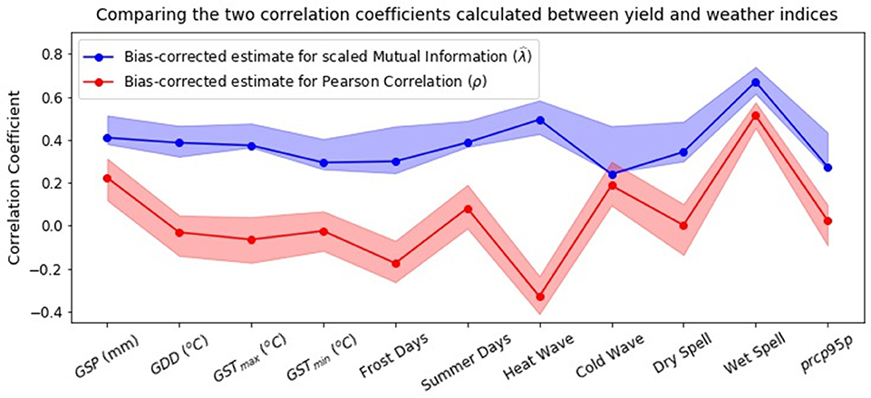
Figure 6. Unbiased estimates for Pearson correlation coefficient (which measures the linear dependence) and scaled Mutual Information (which measures the overall dependence) between corn yield and weather indices. The shaded regions represent the 90% confidence bounds (5% and 95% quantiles) for the unbiased estimates calculated using jackknife resampling. The information contained in certain extreme weather indices, like Summer Days, Heat Wave Index, Longest Dry Spell and Longest Wet Spell is greater than or equal to that contained in the mean weather indices, thus making the case for their inclusion in regression models for predicting crop yield.

The results obtained here indicate a high degree of susceptibility of crop yield to extreme weather, thereby conforming with the key insights from past research (Lobell et al., 2011b, 2013). Many of the previous studies did not include extreme weather indices in their regression models for multiple reasons. The most common being the lack of availability of daily weather data (Lobell et al., 2011b). Also, some of these studies assessed the impact of climate change on crop yield using temperature and precipitation derived from Global Circulation Models (GCMs). The outputs from the current generation of GCMs, however, are usually not thought to be credible at the spatiotemporal resolutions required to directly capture the effect of weather extremes on crop yield. Including extreme weather indices is crucial as they capture the variability of weather within the growing season which is not taken into account in mean weather indices. For example, the same average growing season temperature may arise from two very different seasons, one with little temperature variation and the other with wide fluctuations in temperature. A growing season with widely varying temperatures can result in an increased exposure to extreme conditions, which may critically impact the yields. The insights from this work also agree with those from a different study on the negative impact of temperatures on crop yield (Zhao et al., 2017), which state that with each °C increase in global mean temperature, the global maize yield would reduce by about 7.4% (without any consideration of adaptation strategies or effects of CO₂ fertilization).

Table 2 compares the performance of linear and nonlinear regression models based on metrics like R² and RMSE. For the linear models, PCR and Ridge regression were found to have R² values of 0.89 and 0.88, respectively and RMSE values of 0.32 and 0.33, respectively. Nonlinear regression methods like SVR and Random Forest were found to have slightly better performance. R² values were 0.90 and 0.93 for SVR and Random Forest, respectively with the corresponding RMSE values being 0.32 and 0.25. Overall, Random Forest regression was found to have the best R² and RMSE. This could be attributed to its robustness to data with multicollinearity and for being adept at capturing non-linear interactions. The existence of nonlinear relationships between crop yield and weather indices is not newfound and have been conformed by multiple studies in the past (Schlenker and Roberts, 2009; Lobell et al., 2011a).

TABLE 2

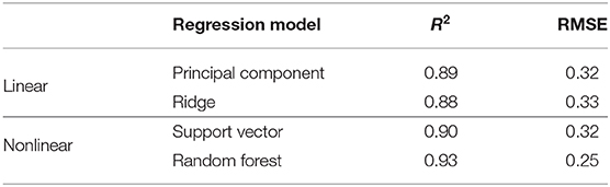
Table 2. Comparison of linear and nonlinear regression approaches to model crop yield using weather indices.

Results from this study could help researchers interested in understanding the impact of environmental factors on crop production. Mechanistic crop simulation models have been traditionally used to model crop growth and yield and to understand patterns of crop yield response to climate change. However, gaps exist in our understanding of crop growth and development processes. One example being the effect of extreme temperatures on crop growth. Asseng et al. (2013) simulated climate change impacts on future global wheat yields and concluded that a greater proportion of the uncertainty was due to variations among mechanistic crop models than to variations among downscaled climate models. Insights from this study could contribute toward a better understanding of the relevant predictors in crop yield modeling and improve our existing knowledge on the precise nature of crop-weather relationship.

Future studies should focus on expanding the scope of this study in terms of the number of crops considered and the spatial extent of the study. When performing this analysis for a broader region, care should be taken to include effects, such as spatial autocorrelation of environmental variables. The presence/absence of irrigation has been shown to negate some of the effects of extreme heat stress on crop growth (Siebert et al., 2017) and hence, should also be considered. There are several limitations of this study. First, the way in which some of the weather indices are computed can have a sizeable impact on the results. A separate analysis was performed to test the sensitivity of some of the extreme weather indices to the specific value of thresholds, as shown in Figures S1, S2. With a couple of indices as test cases (Summer Days and pth percentile precipitation), it was found that the value of threshold used can have a huge impact on the value of the index. This is a problem that has also been acknowledged in previous studies. According to Tack et al. (2015), when calculating growing degree days, including information on the distribution of temperature within each day provides a statistically significant improvement in capturing yield variability. For this particular study, data on intraday variability in temperature was not available and therefore not used. Second, different crop growth stages have different sensitivities to an extreme event. Although this study did include extreme weather indices, it did not consider the specific crop growth stage affected by it. Third, this study included only temperature and precipitation-based indices. However, other environmental factors like relative humidity, ozone and CO₂ concentration have also been shown to affect yield.

6. Conclusions

Changes in the mean and extreme weather pose a major risk to governments and businesses all across the globe. With corn as a test case, the aim of this study was to come up with a systematic approach to understand the nature of the crop yield-weather relationship and determine if extreme weather indices are relevant for yield modeling. Using Mutual Information as a metric for pairwise dependence, it can be concluded that the yield-weather relationship is indeed nonlinear. The information contained in certain extreme weather indices like Summer days, Heat Wave index, Longest Dry spell and Longest Wet Spell was found to be greater than or equal to that contained in the mean weather indices, thus making a case for their inclusion as predictors in crop yield modeling. The results also suggest that Mutual Information can be a better metric for covariate selection over Pearson correlation coefficient as it gives a measure of the overall relationship (linear and nonlinear) between the predictor and response variables. Using a combination of mean and extreme weather indices as inputs, the nonlinear regression models were found to have a slightly better fit than the linear models, with the Random Forest regression giving the best fit and least error on the test set. Future studies should focus on expanding the scope of this analysis, both in terms of the spatial scale and number of crops considered. The implications of this work are important for researchers, businesses and government agencies and especially for platforms like NASA Earth Exchange which facilitate the generation and dissemination of impacts relevant weather data and indices using a multitude of satellite-derived datasets and model outputs.

Data Availability Statement

The data that support the findings of this study are openly available at https://www.ncdc.noaa.gov/cdo-web/ and https://quickstats.nass.usda.gov/.

Author Contributions

VK, TV, SG, and AG contributed to the conceptualization of this study. VK, TV, and AG contributed to the methodology. VK led the preparation of the manuscript with guidance from AG. VK, TV, and AG edited the manuscript.

Funding

Funding for this work was provided by four National Science Foundation (NSF) projects, namely NSF BIGDATA under grant number 1447587, NSF CyberSEES under grant number 1442728, NSF CISE Expeditions in Computing under grant number 1029711 and NSF CRISP type 2 under grant number 1735505. This work was also supported by NASA Earth Exchange.

Conflict of Interest

The authors declare that the research was conducted in the absence of any commercial or financial relationships that could be construed as a potential conflict of interest.

Acknowledgments

The authors would like to thank the data providers including NOAA, USDA NASS, and the reviewers for providing valuable feedback and suggestions.

Supplementary Material

The Supplementary Material for this article can be found online at: https://www.frontiersin.org/articles/10.3389/fsufs.2020.00052/full#supplementary-material

References

Asseng, S., Ewert, F., Rosenzweig, C., Jones, J. W., Hatfield, J. L., Ruane, A. C., et al. (2013). Uncertainty in simulating wheat yields under climate change. Nat. Clim. Change 3, 827–832. doi: 10.1038/nclimate1916

CrossRef Full Text | Google Scholar

Awad, M., and Khanna, R. (2015). “Support vector regression,” in Efficient Learning Machines (New York, NY: Springer), 67–80. doi: 10.1007/978-1-4302-5990-9

CrossRef Full Text | Google Scholar

Breiman, L. (1996). Bagging predictors. Mach. Learn. 24, 123–140. doi: 10.1007/BF00058655

CrossRef Full Text | Google Scholar

Breiman, L. (2001). Random forests. Mach. Learn. 45, 5–32. doi: 10.1023/A:1017934522171

CrossRef Full Text | Google Scholar

Breiman, L., Friedman, J., Olshen, R., and Stone, C. (1984). Classification and Regression Trees. Dordrecht: Taylor & Francis.

Brisson, N., Gate, P., Gouache, D., Charmet, G., Oury, F.-X., and Huard, F. (2010). Why are wheat yields stagnating in Europe? A comprehensive data analysis for France. Field Crops Res. 119, 201–212. doi: 10.1016/j.fcr.2010.07.012

CrossRef Full Text | Google Scholar

Bruinsma, J. (2009). “The resource outlook to 2050: by how much do land, water and crop yields need to increase by 2050,” in Expert Meeting on How to Feed the World in, Vol. 2050 (Rome), 24–26.

Google Scholar

Deryng, D., Conway, D., Ramankutty, N., Price, J., and Warren, R. (2014). Global crop yield response to extreme heat stress under multiple climate change futures. Environ. Res. Lett. 9:034011. doi: 10.1088/1748-9326/9/3/034011

CrossRef Full Text | Google Scholar

Fraser, A. M., and Swinney, H. L. (1986). Independent coordinates for strange attractors from mutual information. Phys. Rev. A 33:1134. doi: 10.1103/PhysRevA.33.1134

PubMed Abstract | CrossRef Full Text | Google Scholar

Gourdji, S. M., Sibley, A. M., and Lobell, D. B. (2013). Global crop exposure to critical high temperatures in the reproductive period: historical trends and future projections. Environ. Res. Lett. 8:024041. doi: 10.1088/1748-9326/8/2/024041

CrossRef Full Text | Google Scholar

Granger, C., and Lin, J.-L. (1994). Using the mutual information coefficient to identify lags in nonlinear models. J. Time Series Anal. 15, 371–384. doi: 10.1111/j.1467-9892.1994.tb00200.x

CrossRef Full Text | Google Scholar

Hoerl, A. E., and Kennard, R. W. (1970). Ridge regression: biased estimation for nonorthogonal problems. Technometrics 12, 55–67. doi: 10.1080/00401706.1970.10488634

CrossRef Full Text | Google Scholar

IPCC (2013a). Climate Change 2014: Impacts, Adaptation, and Vulnerability. Part A: Global and Sectoral Aspects. Contribution of Working Group II to the Fifth Assessment Report of the Intergovernmental Panel on Climate Change. Cambridge; New York, NY: Cambridge University Press, 485–533.

IPCC (2013b). Summary for Policymakers, Book Section SPM. Cambridge; New York, NY: Cambridge University Press, 1–30.

Google Scholar

Joe, H. (1989). Relative entropy measures of multivariate dependence. J. Am. Stat. Assoc. 84, 157–164. doi: 10.1080/01621459.1989.10478751

CrossRef Full Text | Google Scholar

Jolliffe, I. T. (1986). “Principal components in regression analysis,” in Principal Component Analysis (New York, NY: Springer), 129–155. doi: 10.1007/978-1-4757-1904-8

CrossRef Full Text | Google Scholar

Karl, T. R., Nicholls, N., and Ghazi, A. (eds.). (1999). “Clivar/GCOS/WMO workshop on indices and indicators for climate extremes workshop summary,” in Weather and Climate Extremes (Dordrecht: Springer), 3–7. doi: 10.1007/978-94-015-9265-9

CrossRef Full Text | Google Scholar

Khan, S., Ganguly, A. R., Bandyopadhyay, S., Saigal, S., Erickson, D. J., Protopopescu, V., et al. (2006). Nonlinear statistics reveals stronger ties between ENSO and the tropical hydrological cycle. Geophys. Res. Lett. 33:L24402. doi: 10.1029/2006GL027941

CrossRef Full Text | Google Scholar

Kuhn, M., and Johnson, K. (2013). Applied Predictive Modeling, Vol. 26. New York, NY: Springer. doi: 10.1007/978-1-4614-6849-3

CrossRef Full Text | Google Scholar

Lesk, C., Rowhani, P., and Ramankutty, N. (2016). Influence of extreme weather disasters on global crop production. Nature 529:84. doi: 10.1038/nature16467

PubMed Abstract | CrossRef Full Text | Google Scholar

Lobell, D. B., Bänziger, M., Magorokosho, C., and Vivek, B. (2011a). Nonlinear heat effects on African maize as evidenced by historical yield trials. Nat. Clim. Change 1, 42–45. doi: 10.1038/nclimate1043

CrossRef Full Text | Google Scholar

Lobell, D. B., and Burke, M. B. (2010). On the use of statistical models to predict crop yield responses to climate change. Agric. For. Meteorol. 150, 1443–1452. doi: 10.1016/j.agrformet.2010.07.008

CrossRef Full Text | Google Scholar

Lobell, D. B., and Field, C. B. (2011). California perennial crops in a changing climate. Clim. Change 109, 317–333. doi: 10.1007/s10584-011-0303-6

CrossRef Full Text | Google Scholar

Lobell, D. B., Hammer, G. L., McLean, G., Messina, C., Roberts, M. J., and Schlenker, W. (2013). The critical role of extreme heat for maize production in the United States. Nat. Clim. Change 3:497. doi: 10.1038/nclimate1832

CrossRef Full Text | Google Scholar

Lobell, D. B., Schlenker, W., and Costa-Roberts, J. (2011b). Climate trends and global crop production since 1980. Science 333, 616–620. doi: 10.1126/science.1204531

PubMed Abstract | CrossRef Full Text | Google Scholar

MacKay, D. J. (2003). Information Theory, Inference and Learning Algorithms. Cambridge: Cambridge University Press.

Google Scholar

Menne, M. J., Durre, I., Vose, R. S., Gleason, B. E., and Houston, T. G. (2012). An overview of the global historical climatology network-daily database. J. Atmos. Ocean. Technol. 29, 897–910. doi: 10.1175/JTECH-D-11-00103.1

CrossRef Full Text | Google Scholar

Moon, Y.-I., Rajagopalan, B., and Lall, U. (1995). Estimation of mutual information using kernel density estimators. Phys. Rev. E 52:2318. doi: 10.1103/PhysRevE.52.2318

PubMed Abstract | CrossRef Full Text | Google Scholar

Moore, F. C., and Lobell, D. B. (2014). Adaptation potential of European agriculture in response to climate change. Nat. Clim. Change 4:610. doi: 10.1038/nclimate2228

CrossRef Full Text | Google Scholar

NOAA (2018). Climate Data Online. National Climatic Data Center (accessed April 30, 2018).

Osborne, T. M., and Wheeler, T. R. (2013). Evidence for a climate signal in trends of global crop yield variability over the past 50 years. Environ. Res. Lett. 8:024001. doi: 10.1088/1748-9326/8/2/024001

CrossRef Full Text | Google Scholar

Otto, F. E., Massey, N., Oldenborgh, G., Jones, R., and Allen, M. (2012). Reconciling two approaches to attribution of the 2010 Russian heat wave. Geophys. Res. Lett. 39:L04702. doi: 10.1029/2011GL050422

CrossRef Full Text | Google Scholar

OECD and Food and Agriculture Organization of the United Nations (2012). OECD-FAO Agricultural Outlook 2012. 286. doi: 10.1787/agr_outlook-2012-en

CrossRef Full Text | Google Scholar

Pedregosa, F., Varoquaux, G., Gramfort, A., Michel, V., Thirion, B., Grisel, O., et al. (2011). Scikit-learn: machine learning in Python. J. Mach. Learn. Res. 12, 2825–2830. Available online at: http://jmlr.org/papers/v12/pedregosa11a.html

Google Scholar

Ray, D. K., Gerber, J. S., MacDonald, G. K., and West, P. C. (2015). Climate variation explains a third of global crop yield variability. Nat. Commun. 6:5989. doi: 10.1038/ncomms6989

PubMed Abstract | CrossRef Full Text | Google Scholar

Ray, D. K., Mueller, N. D., West, P. C., and Foley, J. A. (2013). Yield trends are insufficient to double global crop production by 2050. PLoS ONE 8:e66428. doi: 10.1371/journal.pone.0066428

PubMed Abstract | CrossRef Full Text | Google Scholar

Ray, D. K., Ramankutty, N., Mueller, N. D., West, P. C., and Foley, J. A. (2012). Recent patterns of crop yield growth and stagnation. Nat. Commun. 3, 1–7. doi: 10.1038/ncomms2296

PubMed Abstract | CrossRef Full Text | Google Scholar

Schauberger, B., Archontoulis, S., Arneth, A., Balkovic, J., Ciais, P., Deryng, D., et al. (2017). Consistent negative response of US crops to high temperatures in observations and crop models. Nat. Commun. 8, 1–9. doi: 10.1038/ncomms13931

PubMed Abstract | CrossRef Full Text | Google Scholar

Schlenker, W., and Roberts, M. J. (2009). Nonlinear temperature effects indicate severe damages to US crop yields under climate change. Proc. Natl. Acad. Sci. U.S.A. 106, 15594–15598. doi: 10.1073/pnas.0906865106

CrossRef Full Text | Google Scholar

Siebert, S., Webber, H., Zhao, G., and Ewert, F. (2017). Heat stress is overestimated in climate impact studies for irrigated agriculture. Environ. Res. Lett. 12:054023. doi: 10.1088/1748-9326/aa702f

CrossRef Full Text | Google Scholar

Smola, A. J., and Schölkopf, B. (2004). A tutorial on support vector regression. Stat. Comput. 14, 199–222. doi: 10.1023/B:STCO.0000035301.49549.88

CrossRef Full Text | Google Scholar

Tack, J., Barkley, A., and Nalley, L. L. (2015). Effect of warming temperatures on US wheat yields. Proc. Natl. Acad. Sci. U.S.A. 112, 6931–6936. doi: 10.1073/pnas.1415181112

PubMed Abstract | CrossRef Full Text | Google Scholar

Tilman, D., Balzer, C., Hill, J., and Befort, B. L. (2011). Global food demand and the sustainable intensification of agriculture. Proc. Natl. Acad. Sci. U.S.A. 108, 20260–20264. doi: 10.1073/pnas.1116437108

PubMed Abstract | CrossRef Full Text | Google Scholar

Troy, T., Kipgen, C., and Pal, I. (2015). The impact of climate extremes and irrigation on US crop yields. Environ. Res. Lett. 10:054013. doi: 10.1088/1748-9326/10/5/054013

CrossRef Full Text | Google Scholar

Urban, D., Roberts, M. J., Schlenker, W., and Lobell, D. B. (2012). Projected temperature changes indicate significant increase in interannual variability of US maize yields. Clim. Change 112, 525–533. doi: 10.1007/s10584-012-0428-2

CrossRef Full Text | Google Scholar

USDA (2010). Quick Stats NASS USDA (accessed April 30, 2018).

Vapnik, V. (2013). The Nature of Statistical Learning Theory. New York, NY: Springer Science & Business Media.

Google Scholar

Vapnik, V. N. (1995). The Nature of Statistical Learning Theory. New York, NY: Springer-Verlag.

Google Scholar

Zhao, C., Liu, B., Piao, S., Wang, X., Lobell, D. B., Huang, Y., et al. (2017). Temperature increase reduces global yields of major crops in four independent estimates. Proc. Natl. Acad. Sci. U.S.A. 114, 9326–9331. doi: 10.1073/pnas.1701762114

PubMed Abstract | CrossRef Full Text | Google Scholar