Methane emissions from California dairies estimated using novel climate metric Global Warming Potential Star show improved agreement with modeled warming dynamics

1. Introduction

CH₄ has the second greatest radiative forcing of all anthropogenic GHG after CO₂ (Myhre et al., 2013), and global CH₄ emissions, to which livestock is a major contributor, are responsible for about 0.5C of the 1.1C of human-forced global warming which has taken place since the year 1850 (IPCC, 2021). Enteric fermentation in the rumen of dairy cattle and their manure are major sources of biogenic methane (CH₄). Atmospheric CH₄ concentrations have increased by ~150% since pre-industrial time (Gulev et al., 2021). Recent studies suggest that the increasing global CH₄ growth rate since 2007 has in part been driven by biogenic sources (Kai et al., 2011; Nisbet et al., 2016; Schaefer et al., 2016; Schwietzke et al., 2016).

CO₂ is known as a “cumulative pollutant” or “stock gas” due to its atmospheric lifetime that ranges from centuries to millennia (Pierrehumbert, 2014), causing it to accumulate in the atmosphere. CH₄, on the other hand, is known as a “short-lived climate pollutant” (SLCP) or “flow gas,” and has an e-folding time of about 12 years. When both CO₂ and SLCP emissions increase over time, there is a short-term climate response to the change in radiative forcing (“transient warming”). When SLCP sources and sinks are equal, some long-term “equilibrium warming” will occur while the climate system equilibrates to past increases in SLCP emissions. However, after a sufficiently long period of constant emissions, there is no net accumulation in the atmosphere, radiative forcing of the atmospheric SLCP remains approximately constant, and SLCP-induced warming will stabilize. In contrast, CO₂-induced warming will always increase under positive CO₂ emissions (Cain et al., 2019). Because of its flow nature, a rapid reduction in methane emissions is one of the most feasible short-term measures to immediately curb global temperature rise (Ocko et al., 2021).

Climate metrics are used to “convert” annual emissions of various GHG that differ by atmospheric lifetime, radiative forcing, and relative magnitude of emissions into one common unit. One of the most widely used climate metrics is Global Warming Potential (GWP). GWP is constructed to estimate the radiative forcing of an emission pulse integrated over a given time horizon (often 20 or 100 years) relative to an equivalent pulse of CO₂. As constructed, GWP does not compare CO₂ to CH₄ emissions on the basis of equal radiative forcing, an accepted meaning of emissions equivalence within the radiative forcing framework, and therefore the meaning of emissions equivalence of CO₂ and CH₄ using GWP can be ambiguous (Wigley, 1998). GWP also does not relate radiative forcing to temperature change and as such is not able to capture temperature impacts within cumulative emission frameworks, although it is occasionally used for this purpose (Cui et al., 2017). GWP also does not differentiate between the contrasting behaviors of stock and flow gases, so GWP cannot capture the stable SLCP atmospheric concentrations that result from stable SLCP emissions rates. Because GWP treats SLCP like CO₂, which accumulates in the atmosphere even under stable emissions rates, GWP yields the wrong direction of temperature change under declining SLCP (Lynch et al., 2020). When CO₂ and CH₄ are compared specifically to assess their relative warming impacts on the climate, GWP overstates the warming impact of constant CH₄ emissions on global surface temperature by a factor of 3–4 over a 20-year time horizon, while understating the effect of a new CH₄ emission source by a factor of 4–5 over the 20 years following its introduction (Lynch et al., 2020). IPCC AR6 does not recommend any given emission metric because metric appropriateness depends on the purpose for which gases are being compared.

Because livestock GHG emissions are predominately SLCP, the warming effects of livestock agriculture can be overestimated by GWP (Persson et al., 2015). The choice of the climate metric can change the estimated climate effect of CH₄, creating uncertainties in livestock contributions to global climate change and impacts of GHG mitigation in this sector (Reisinger et al., 2013). Thus, climate metrics designed to assess SLCPs more accurately are essential to quantify the warming impacts of animal agriculture, as well as husbandry factors that control these effects over time, such as increasing efficiency and decreasing herd size. In North America, decreasing dairy herd size and increasing production efficiency may have altered relative sizes of dairy GHG sources and sinks (Capper et al., 2009; Naranjo et al., 2020). California is the largest dairy producer in the United States (USDA National Agricultural Statistics Service, 2019), and in 2017, agricultural manure management was California's second largest source of CH₄. Dairy CH₄ emissions from cow manure in California are relatively high because flush water lagoon systems are the predominate manure management system on California dairies (CARB, 2022b), and anaerobic lagoons emit the most CH₄ per head of all common manure management practices (Owen and Silver, 2015). In 2016, the California Senate passed S.B. 1383, mandating a 40% reduction of dairy manure management CH₄ emissions from 2013 levels by 2030 (Lara, 2016). Thus, using a metric that can capture the flow nature of CH₄ will gain importance as agricultural CH₄ emissions reductions strategies are implemented, particularly those targeting emissions from dairy manure.

In response to potential misrepresentations of warming effects of SLCPs by GWP, an alternate metric, Global Warming Potential Star (GWP^*) has been developed. GWP^* is a recent and novel application of the commonly used climate metric GWP, designed to represent the flow gas properties of SLCP rather than treating them like cumulative stock gases such as CO₂. While applying GWP to annual emissions of non-CO₂ GHG gives emissions in units of “CO₂-equivalent emissions (CO₂eq),” GWP^* gives emissions in “CO₂-warming equivalent emissions (CO₂we).” GWP^* relates CO₂ pulses to SLCP emissions based on approximately equivalent radiative forcing of the emissions, so CO₂we are both directly comparable to CO₂eq and can be directly related to temperature change caused by these emissions (Smith et al., 2021), unlike GWP-based CO₂eq, as discussed above (Wigley, 1998). GWP^* has been demonstrated to capture dynamics of SLCP-forced warming in datasets with global emissions across many economic sectors (Lynch et al., 2020). While some authors have debated the applicability of GWP^*to national and sectoral emissions (Rogelj and Schleussner, 2019), the present study is the first to use GWP^* to assess dairy CH₄ warming dynamics over time and to estimate warming impacts of the mandated CH₄ mitigation efforts in California using GWP vs. GWP^*. While the objective of this study was not to provide a comprehensive inventory of all CH₄ emissions from California dairy production or a cradle-to-farm gate environmental impact analysis of the California dairy production system, the present study serves as a case study to assess GWP^*'s ability to represent the warming effects of sectoral SLCP under declining emissions rates. It also serves as a characterization of potential drivers of these declining dairy CH₄ emissions in California. Our objectives were to compare GWP-based CO₂-equivalent emissions vs. GWP^*-based CO₂-warming equivalent emissions calculated from historical California CH₄ emissions from lactating dairy cattle and to characterize dairy CH₄ warming dynamics from 1990 to 2017. We also aimed to compare the GWP- and GWP^*-based dynamics of warming effects of dairy CH₄ under future business-as-usual and reduction emissions scenarios. We hypothesized that GWP^*-based cumulative CO₂-warming equivalent emissions would decline under declining CH₄ emissions and would match the dynamics of CH₄'s warming effects.

2. Methods

2.1. Estimating annual methane emissions from California dairy cattle

2.1.1. Calculation of historical methane emissions from California dairy cattle (1950–2017)

We calculated annual enteric fermentation and manure management CH₄ emissions from 1950 to 2017 based on the historical California dairy cow population and US EPA Greenhouse Gas Inventory Annex 3.10 (EPA, 2013a). “Annual” emissions refer to yearly CH₄ emissions estimates that have not been converted into CO₂-equivalent or CO₂-warming equivalent emissions. Total annual CH₄ emissions from California dairies were calculated using Equation 1:

$\begin{array}{l}{\text{E}}_{\text{C}{\text{H}}_4}={\text{E}}_{\text{EF}}+{\text{E}}_{\text{MM}}\end{array}$

Where E_CH4is total annual CH₄ emissions (kg CH₄ per year), E_EF is annual enteric fermentation CH₄ emissions (kg CH₄ per year), and E_MM is annual manure management CH₄ emissions (kg CH₄ per year).

Annual CH₄ emissions from enteric fermentation were calculated using Equation 2:

$\begin{array}{l}{\text{E}}_{\text{EF}}=\text{Po}{\text{p}}_{\text{dairy}}\times \text{E}{\text{F}}_{\text{EF}}\end{array}$

Where E_EF is annual enteric fermentation CH₄ emissions (kg CH₄ per year), Pop_dairy is annual lactating dairy cow population (head dairy cow) and EF_EF is annual enteric fermentation emission factor (kg CH₄ per head dairy cow per year).

Dairy cow populations were derived from California Department of Food and Agriculture (CDFA) Agricultural Resource Directory reports, which provided total dairy cattle population data by county (CDFA, 2000, 2007). Annual enteric CH₄ and manure CH₄ emission factors for California dairy cattle for 2000–2017 were obtained from the California Air Resources Board (CARB) Documentation of California's Greenhouse Gas Inventory (CARB, 2022a,b). The CDFA dairy cattle population data was assumed to represent only lactating cows, so we used the enteric fermentation CH₄ emission factor for lactating cows. Enteric CH₄ emissions factors are determined based on estimated gross energy (GE) intake and CH₄ conversion rate (Y_m), which is the fraction of GE in feed converted to CH₄. GE and Y_m depend on the animal's production demands, and the characteristics of the diet fed (EPA, 2013a). Manure CH₄ emissions factors are estimated by CARB using US EPA methodology (EPA, 2013b) and are based on typical animal mass, volatile solids excretion rate (portion of organic matter in the diet that was not digested by the animal and is thus available for use by methanogenic bacteria), maximum methane producing capacity of excreted volatile solids, and nitrogen excretion rate (CARB, 2022b). Because annual emission factors were unavailable before 2000, we used the 2000 emission factors for estimates from 1950 to 1999 (Supplementary Table S1). Annual CH₄ emissions from manure management (E_MM, kg CH₄ per year) were calculated for i different manure management practices (MMP) with emission factor EF_MMPi (kg CH₄ per cow, Supplementary Table S2) using Equation 3:

$\begin{array}{l}{\text{E}}_{\text{MM}}=\text{Po}{\text{p}}_{\text{dairy}}\times \left({\displaystyle \sum _{i=1}^{\text{i}}}\text{E}{\text{F}}_{\text{MM}{\text{P}}_{\text{i}}}\times \frac{\text{manur}{\text{e}}_{\text{MM}{\text{P}}_{\text{i}}}}{\text{manur}{\text{e}}_{\text{total}}}\right)\end{array}$

The proportion of manure managed by each manure management system in California and the emissions factors for each management system were obtained from the Documentation of California's Greenhouse Gas Inventory (CARB, 2022b). Because MMP proportions before year 2000 were not available from CDFA, we used the 2000 manure management practice proportions and emissions factors for 1950–1999 (Supplementary Table S3).

2.1.2. Scenario analysis of methane emissions from California dairy cattle (2018–2029)

Business-as-usual (“BAU”) future emissions scenarios were generated using the same methodology. We obtained projected California dairy cattle population for 2018 to 2029 from the 2020 U.S. Agricultural Market Outlook baseline report from the Agricultural Markets and Policy (AMAP) program at the University of Missouri (FAPRI and AMAP, 2020a), which provides projected dairy cattle population assuming current policies and macroeconomic conditions remain in place (FAPRI and AMAP, 2020b). The model includes behavioral supply equations that determine milk supply via dairy cow inventories and milk yield per cow on a state-level basis. Milk supply equations are driven by expected net returns, which are driven by applicable federal or state policy. Demand equations are specified as a function of price, relevant substitute product prices and consumer income for various milk products (Johnson et al., 1993; Westhoff and Brown, 1999; Blayney and Normile, 2004; Fabiosa et al., 2005). These dairy cattle population projections (Supplementary Table S4) have an average annual decline rate of 0.32%, which agrees with CARB estimates of 0.5% decline in dairy cattle population from 2017 onward (CARB, 2022c). We assumed all cows in the projected dairy cattle population were lactating. We used 2017 emission factors and MMPs to calculate emissions from these dairy cows and used these emissions to extend historical 1950–2017 emissions time series to 2029 under “business-as-usual,” meaning with no methane reduction programs. We used 2017 emissions factors because projected emissions factors were not available. Enteric fermentation emissions factors used by CARB were the same from 2012 to 2017 (Supplementary Table S1). Furthermore, the same emissions factors have been used up to 2020, the most recent year of the CARB GHG emissions inventory (CARB, 2022a). Because CH₄ emissions factors are estimated based on dietary and production parameters, if regionally typical diets and production remain approximately the same over time, emissions factors will remain the same from year to year. Thus, without data on future dairy cattle enteric CH₄ emissions factors, we assumed that enteric fermentation CH₄ emissions per cow would remain stable through 2029. See Section 4.4 for further exploration of this assumption.

Because AMAP provided historical cattle population data that differed slightly from the CDFA population data used for annual CH₄ emissions, enteric fermentation and manure management CH₄ emissions estimates from both differed. Linear regression was used to relate enteric fermentation and manure management CH₄ emissions estimates based on historical AMAP and CDFA population values from years for which estimates for both were available, and then future emissions estimates based on AMAP population values were adjusted according to the regression relationship (see Supplementary Table S4 for further explanation).

We generated the “Manure 40” emissions reduction scenario following California Senate Bill No. 1383 which mandates the adoption of “regulations to reduce methane emissions from livestock manure management operations and dairy manure management operations, consistent with this section and the strategy, by up to 40 percent below the dairy sector's and livestock sector's 2013 levels by 2030” (Lara, 2016). This law requires reductions in manure management emissions and does not mandate reductions in enteric fermentation emissions, so the aggregated scenario “Manure 40 plus BAU EF” refers to the manure management 40% reduction scenario added to the “business as usual” enteric fermentation (BAU EF) scenario. We assumed the 40 percent reduction goal would be met by 2030 and assumed a constant rate of reduction to meet these goals from 2018 to 2030. Such reductions could potentially be achieved by converting manure management systems from high-CH₄ emitting anaerobic lagoons to alternative management systems; see Section 2.4. Methane emissions between 2017 and 2030 were interpolated with constant reduction rate; the difference between emissions in 2017 and 2030 was divided by 13 and this step value was added to each intervening year. We also generated the “3NOP” enteric fermentation reduction scenario using reductions from use of 3-nitroxypropanol (3NOP), a synthetic feed additive that inhibits the enzyme that catalyzes the methane-forming step in the rumen (Duin et al., 2016). Maximum reductions in enteric CH₄ emissions from dairy cattle supplemented with 3NOP vary across studies and may depend on animal factors and basal diet (Dijkstra et al., 2018). In the only dairy 3-NOP study conducted in California, maximum net reductions using 3NOP were 11.7% (Feng and Kebreab, 2020). We assumed this reduction would be achieved by 2030 and interpolated emissions of intervening years using the same method as manure management emissions. The “Manure 40 plus 3NOP” refers to the 40% manure management reduction scenario plus the 11.7% “3NOP” enteric fermentation reduction scenario.

2.2. Calculating CO₂-equivalent emissions using GWP and CO₂-warming equivalent emissions using GWP^*

2.2.1. Converting annual CH₄ emissions to CO₂-equivalent emissions using GWP

In the following section, we describe how GWP and GWP^* were used to calculate CO₂-equivalent (CO₂eq) or CO₂-warming equivalent emissions (CO₂we), respectively. GWP is generated by integrating the radiative forcing (the change in incoming and outgoing energy of the Earth system actuated by a given GHG) of a single emission (“pulse”) of that GHG over a given time horizon H, divided by the same quantity for CO₂. The GWP of gas i with radiative forcing (RF_i) by Equation 4:

$GW{P}_i=\frac{{\displaystyle {\int }_0^{H}R{F}_i(t)}dt}{{\displaystyle {\int }_0^{H}R}{F}_{C{O}_2}(t)dt}$

(Solomon et al. 2007).

GWP is used to convert other GHGs into CO₂eq, defined for a gas i as emissions per year (E_i) multiplied by GWP. CO₂eq are defined by Equation 5:

$\begin{array}{l}C{O}_{2}eq=E_i\times GW{P}_i.\end{array}$

Where CO₂eq are given in teragrams per year (Tg, equivalent to million metric tons, MMT) of CO₂eq emissions (TgCO₂eq/year) and E_i is given in Tg per year of gas E_i.

We used a 100-year time horizon for both GWP and GWP^*. We used the GWP₁₀₀value of CH₄ from the IPCC 4th Assessment Report (Solomon et al., 2007), 25, which is consistent with the CARB GHG Current California Emission Inventory Data (CARB, 2022a,b).

2.2.2. Converting annual CH₄ emissions to CO₂-warming equivalent emissions using GWP^*

We converted the CH₄ emissions into CO₂-warming equivalent emissions (CO₂we) using GWP^*. GWP^* considers an increase in the emission rate of an SLCP to be equivalent to a one-off pulse emission of CO₂ (Allen et al., 2018) and is used to convert SLCP emissions to CO₂we, which are directly comparable to CO₂eq (Allen et al., 2018). Under GWP^*, CO₂we are defined by Equation 6:

$\begin{array}{l}C{O}_{2}we=GW{P}_i\times \left(r\times \frac{d{E}_i}{dt}\times H+s\times E_i\right)\end{array}$

where CO₂we are given in Tg of CO₂-warming equivalent emissions per year (TgCO₂we per year), GWP_i is the conventional GWP for gas i over time-horizon H, dE_i the change in the emission rate of gas i over the preceding dt years in Tg E_i per year, E_i the emissions of gas i in that year in Tg E_i per year, and r and s the weights assigned to the rate and stock contributions, respectively (Cain et al., 2019). r controls the rate-dependent warming effects of SLCP and s controls the long-term equilibration to past increases in forcing. We used r = 0.75 and s = 0.25 according to Cain et al. (2019), where these coefficients are the mean of coefficients determined when regressing different cumulative CH₄ emissions scenarios against modeled warming of these emission scenarios. We used a dt of 20 years according to Allen et al. (2018). Using r = 0.75, s = 0.25, H = 100, and dt = 20, the GWP^* equation can be simplified further to Equation 7 (Lynch et al., 2020):

$\begin{array}{l}C{O}_{2}we=(4\times E_{i_t}-3.75\times E_{i_{t-20}})\times GW{P}_i.\end{array}$

We used this equation for conversion of annual CH₄ emissions into CO₂we emissions. It should be noted that the definition of GWP^*-based CO₂-warming equivalent emissions has since been updated to include a scaling factor g (g = 1.13) to directly relate the radiative forcing of CO₂ and SLCP emissions without reference to temperature response, but the authors suggest that scaling factors of order 10% may not be necessary given their additional complexity (Smith et al., 2021).

2.3. Modeling warming responses to estimated methane emissions

We used the FaIR (Finite-Amplitude Impulse Response) v1.3 climate-carbon-cycle model to simulate the warming effects of the annual CH₄ emissions (Millar et al., 2017; Smith et al., 2018). It should be noted that this FaIR model is not the same as climate policy decision-support tool FAIR model (den Elzen and Lucas, 2005). Following Lynch et al. (2020), we forced the model with the complete RCP4.5 emissions scenario (Smith and Wigley, 2006; Wise et al., 2009; Lamarque et al., 2010), then forced the model with these same emissions, plus CH₄ emissions from each scenario. We then subtracted the first warming time-series from the second to generate the warming response to each emissions scenario. We used default FaIR parameters and set volcanic and solar forcing to zero and efficacies for each forcing agent compared to CO₂ to one, except black carbon, which was set to three (Bond et al., 2013).

2.4. Identifying husbandry factors driving declining dairy CH₄ emissions

Given the importance of capturing CH₄'s flow nature especially under declining emissions rates, we conducted a separate analysis from that described in Sections 2.1–2.3 to determine if California dairy background CH₄ emissions are declining and identify husbandry factors driving potential decline. Production data (dairy cattle populations and per capita dairy cow milk production) were obtained from the USDA QuickStats database (USDA National Agricultural Statistics Service, 2019). Manure management CH₄ reductions from emissions reduction programs were obtained from the CDFA Dairy Digester Research and Development Program (DDRDP) and Alternative Manure Management Program (AMMP) websites (CDFA, 2022a,b). To investigate the impact of these programs, we estimated what CH₄ emissions would have hypothetically been without these programs. These estimates comprised a separate analysis and were not used to investigate emission dynamics or to force the climate model but were only used to assess the impact of various factors that may have led to reduced CH₄ emissions in California. To estimate hypothetical emissions without DDRDP and AMMP, annual emission reductions provided by CDFA were converted from Tg CO₂eq to Tg CH₄ using the AR4 GWP100 of CH₄ (25) and were added cumulatively to the estimated total annual dairy CH₄ emissions of the reduction year. For example, the 2016 estimated emissions reductions were added to 2016 CH₄ emissions to estimate hypothetical 2016 emissions without DDRDP or AMMP reductions, and 2016 plus 2017 estimated emissions reductions were added to 2017 CH₄ emissions to estimate putative 2017 emissions without DDRDP or AMMP reductions, etc. Although DDRDP and AMMP reductions were available to 2019, historical CH₄ emissions were only available to 2017, so the 2017 CH₄ emissions were used for all years following 2017. Statistical analysis for the entire study was conducted in R (R Core Team, 2020).

3. Results

3.1. Comparison of average annual CO₂eq and CO₂we from each scenario

We converted historical annual CH₄ emissions, a future business-as-usual CH₄ emission scenario, and two future reduction CH₄ emissions scenarios from California dairy cattle into CO₂-equivalent emissions or CO₂-warming equivalent emissions using the two different metrics GWP and GWP^*, respectively. We used the conventional GWP and the novel GWP^*, which is a modification of GWP that contains a term for the change in the rate of emission of SLCP such as methane. GWP gives CO₂-equivalent emissions (CO₂eq), while GWP^* gives CO₂-warming equivalent emissions (CO₂we). “Total dairy emissions” were calculated using Equation 1. We used an emission-based climate model to predict the warming impacts of each annual CH₄ emissions scenario to compare the warming profiles against the dynamics of CO₂-equivalent emissions calculated by each metric for each scenario.

We first investigated if GWP-based emissions estimates (CO₂eq) and GWP^*-based emissions estimates (CO₂we) differed significantly in each emissions scenario. GWP-based CO₂eq emissions and GWP^*-based CO₂we were calculated from identical annual “background” CH₄ emissions, but all average CO₂eq and CO₂we under the same reduction scenarios differed significantly (Figure 1). Average GWP^*-based estimates for the historical period were larger than GWP-based estimates. In this historical period, there are 37% more annual CO₂-warming equivalent CH₄ emissions when calculated using GWP^* than when calculated using GWP (Figure 1).

FIGURE 1

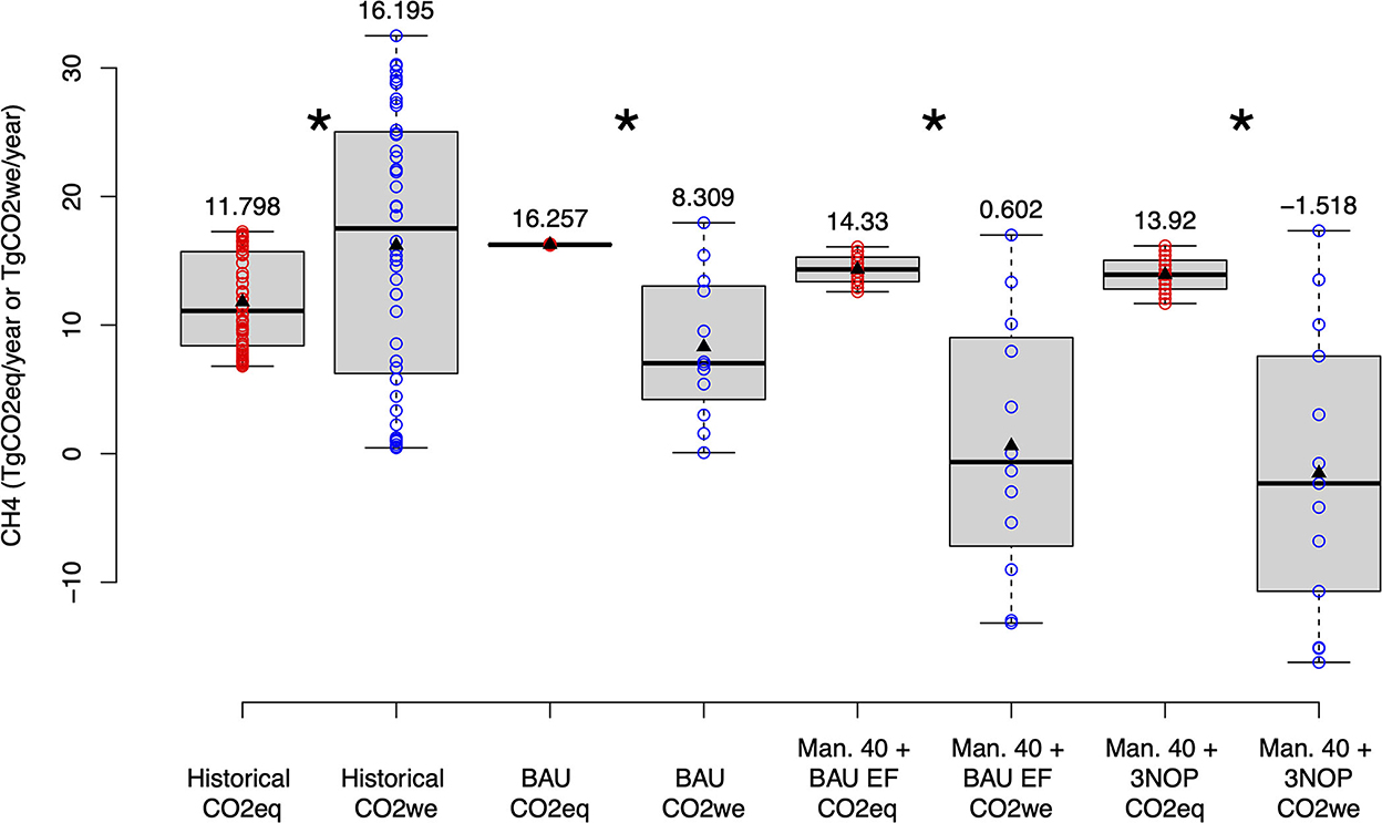
Figure 1. Comparison of annual total dairy CH₄ emissions converted to CO₂eq and CO₂we using GWP and GWP*, respectively. The x-axis shows each emission scenario and which metric was used. Historical data is from 1950 to 2017. The BAU scenario and Manure 40 plus BAU EF (“Man. 40 + BAU EF”) are from 2018 to 2029. The Manure 40 plus 3NOP (“Man. 40 + 3NOP”) is from 2018 to 2030. The y-axis denotes CO₂-equivalent or CO₂-warming equivalent emissions, respectively, computed from CH₄ emissions; GWP gives “CO₂eq” emissions, while GWP* gives “CO₂we.” Each circle represents an observation of annual emissions rate from each time period and emissions scenario. Red open circles are data points calculated using GWP; blue open circles are data points calculated using GWP*. Values above boxes are mean values; means are denoted as black triangles on plot. Asterisks between plots indicate means of GWP- and GWP*-based emissions differ significantly (paired student's t-test, p < 0.05).

In the BAU manure and enteric CH₄ scenario and 40% reduction of manure management CH₄ with BAU enteric CH₄ scenario, CO₂we were lower than CO₂eq (Figure 1). Furthermore, under 40% reduction of future annual manure management CH₄ emissions in the “Man. 40 plus BAU EF CO2eq” reduction scenario, some annual CO₂we are negative, while CO₂eq were never negative. Under 40% reduction of future annual manure management CH₄ emissions with maximum 3NOP reductions, the average of all annual CO₂we were negative, while again CO₂eq were never negative (Figure 1).

CO₂eq are less variable than GWP^*-based CO₂ warming equivalent emissions, particularly in the future BAU scenario, where CO₂eq are approximately constant. GWP^*-derived emissions are more variable because they are calculated by subtracting the current year emissions rate from that of 20 years previously, which is particularly variable under reduction scenarios where future emissions are reduced relative to those in the historical period.

3.2. Comparison of cumulative CO₂eq and CO₂we with modeled warming over historical period (1950–2017)

Because cumulative CO₂ emissions and temperature change are linearly related (Allen et al., 2009; Matthews et al., 2009), the dynamics of the two should be similar over time and the warming profile serves as a means of evaluating GWP and GWP^*. We next examined the relationship between “background” annual CH₄ emissions, cumulative GWP- and GWP^*-based emissions estimates, and modeled warming, in each emissions scenario, to evaluate these two metrics.

In the historical period, annual CH₄ emissions increased from 1950 to 2008, but slightly decreased from 2008 to 2017 (Figure 2A). During the increasing annual CH₄ emissions, CO₂we were higher than CO₂eq (Figure 2B). Under decreasing annual CH₄ emissions from 2008 to 2017, however, annual CO₂we decreased, while annual CO₂eq increased. Because annual CO₂we decreased from 2008 to 2017, when each annual estimate was added up to give cumulative emissions, cumulative CO₂we did not increase linearly from 2008 to 2017 but instead, the rate of increase of cumulative emissions slowed, decreasing the slope of the line (Figure 2C). In contrast, because annual CO₂eq increased over the entire historical period, cumulative CO₂eq increased linearly (Figure 2C). The slope of the line representing warming caused by annual CH₄ emissions also decreased from 2008 to 2017 (Figure 2C). As noted above, the dynamics of cumulative CO₂-equivalent emissions and warming forced by these emissions should be similar over time, so in this scenario, the decreasing slope of the warming and cumulative GWP^* lines suggests that they may be in better agreement than GWP and the warming line.

FIGURE 2

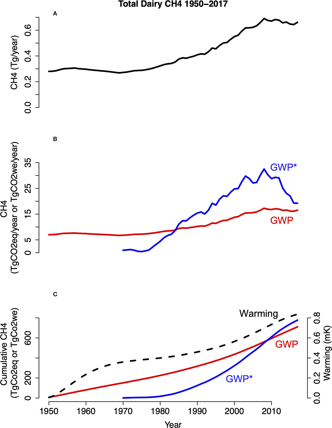
Figure 2. California 1950–2017 total historical CH₄ emissions, comparison of these emissions converted to CO₂eq and CO₂we using GWP and GWP*, respectively, and cumulative CO₂eq and CO₂we with emissions-forced warming. The x-axis represents years and the y-axis represents annual CH₄ emissions (A), annual CO₂eq or CO₂we (B), or cumulative CO₂eq or CO₂we (C). CO₂we are represented in (B, C) by the blue solid line (“GWP*”), GWP-based CO₂eq are represented by the red solid line (“GWP”), and temperature is given in (C) by the dashed black line (“Warming”). The temperature axis in (C) is scaled by 0.001 mK/TgCO₂, or 1 K/TtCO₂. The scaling factor that relates cumulative CO₂ emissions to temperature change is known as transient climate response to cumulative carbon emissions (TCRE). The scaling factor here (approximate TCRE) exceeds the IPCC likely range, likely due to a large increase in annual CH₄ emissions in the 1950s leading to a larger GWP of CH₄ in this period (see Section 4). This large GWP may be responsible for the “bulge” in warming between 1950 and 1990 (C).

3.3. Comparison of cumulative CO₂eq and CO₂we with modeled warming over BAU scenario (2017–2029)

In the BAU manure and enteric CH₄ emissions scenario, annual background CH₄ emissions from 2008 to 2029 were approximately constant (Figure 3A). Under constant annual CH₄ emissions, CO₂we declined, while CO₂eq were approximately constant (Figure 3B).

FIGURE 3

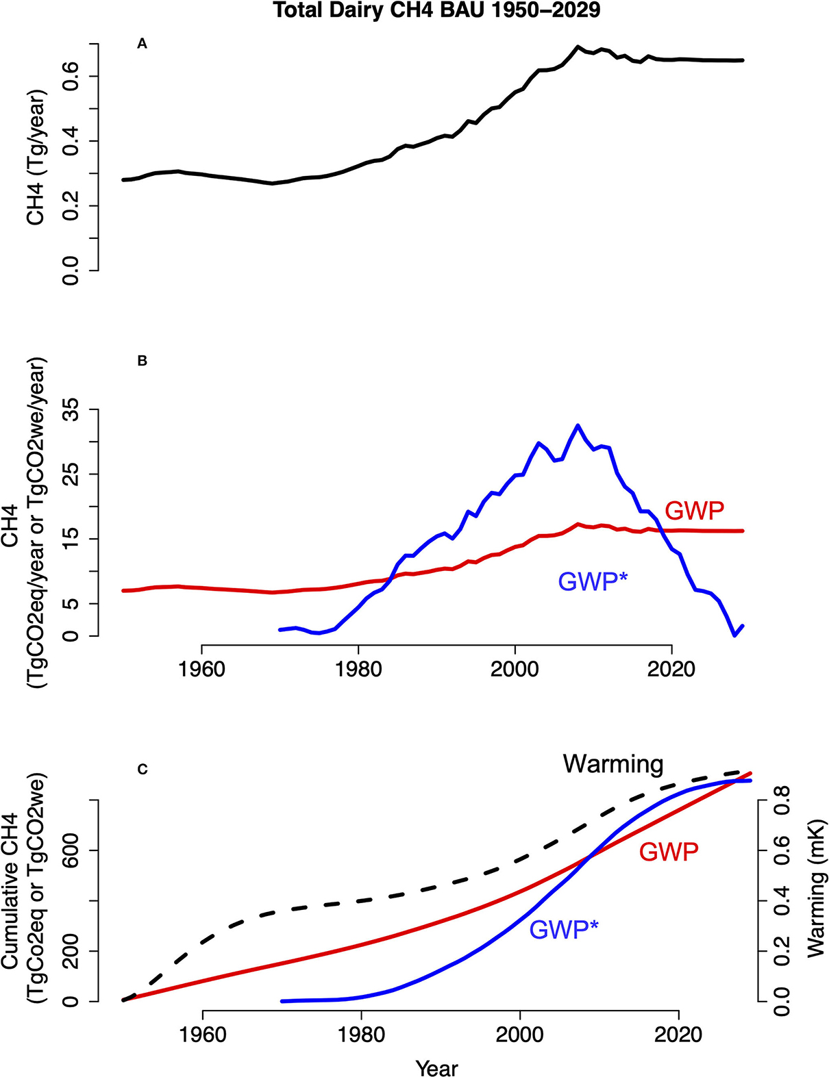
Figure 3. California future BAU total (enteric fermentation plus manure management) CH₄ emissions, comparison of these emissions converted to CO₂eq and CO₂we using GWP and GWP*, respectively, and cumulative CO₂eq and CO₂we with emissions-forced warming. The x-axis represents years and the y-axis represents annual CH₄ emissions (A), annual CO₂eq or CO₂we (B), or cumulative CO₂eq or CO₂we (C). CO₂we are represented in (B, C) by the blue solid line (“GWP*”), CO₂eq are represented by the red solid line (“GWP”), and temperature is given in (C) by the dashed black line (“Warming”). The temperature axis (C) is scaled by 0.001 mK/TgCO₂, or 1 K/TtCO₂, as in Figure 2.

Because annual CO₂we decreased from 2008 to 2017, when each annual estimate was added up to give cumulative emissions, cumulative CO₂we did not increase linearly from 2008 to 2017 but instead, the rate of increase of cumulative emissions slowed and the line representing CO₂we “flattens out,” or stops accumulating (Figure 3C). In contrast, because annual CO₂eq increased over the entire historical period, cumulative CO₂eq increased linearly (Figure 3C).

Because GWP^*-based cumulative CO₂we did not increase under constant annual CH₄ emissions, they fit the warming better than CO₂eq, like in the historical period, but the difference in the near-constant BAU scenario is easier to see. GWP-derived estimates did not match warming dynamics because CO₂eq continued to increase linearly under constant annual CH₄ emissions.

3.4. Comparison of cumulative CO₂eq and CO₂we with modeled warming over 40% manure CH₄ emissions reduction plus BAU enteric CH₄ emissions scenario (2017–2029)

In the “Manure 40 plus BAU EF” reduction scenario, manure CH₄ is reduced by 40% from 2017 to 2029, while enteric CH₄ follows a “business as usual” projection. In this moderate reduction scenario, annual background manure management and total CH₄ emissions declined from 2017 to 2029 (Figures 4A, B). Under declining CH₄ emissions from 2017 to 2029, both manure management and total CO₂we declined, even reaching negative annual emissions rates (Figures 4C, D). CO₂eq also declined under declining annual CH₄ emissions, but did not reach negative emissions rates.

FIGURE 4

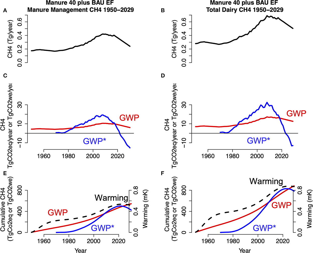
Figure 4. California future manure management and total “Manure 40 plus BAU EF” reduction scenario CH₄ emissions, comparison of these emissions converted to CO₂eq and CO₂we using GWP and GWP*, respectively, and cumulative CO₂eq and CO₂we with emissions-forced warming. The x-axis represents years, and the y-axis represents annual CH₄ emissions (A, B), annual CO₂eq or CO₂we (C, D), and cumulative CO₂eq or CO₂we (E, F). Manure management CH₄ is presented in (A, C, E), and total dairy CH₄ is given by (B, D, F). CO₂we are represented in (C–F) by the blue solid line (“GWP*”), CO₂eq are represented in (C–F) by the red solid line (“GWP”), and temperature is given in (E, F) by the dashed black line (“Warming”). The temperature axis (C) is scaled by 0.001 mK/TgCO₂, or 1 K/TtCO₂, as in previous figures. The horizontal black line in (C, D) is at y = 0.

When each annual CO₂we emissions estimate was added up to give cumulative emissions, because some annual emissions rates were negative, cumulative CO₂we decreased from 2017 to 2029 (Figures 4E, F). In contrast, GWP-based cumulative CO₂eq continued to increase under declining future annual CH₄ emissions (Figures 4C, D). Warming forced by declining annual CH₄ emissions also declined, so cumulative GWP^*-based CO₂we reflected these dynamics better than cumulative GWP-based CO₂eq.

3.5. Comparison of cumulative CO₂eq and CO₂we with modeled warming over 40% manure CH₄ emissions reduction plus reduced enteric CH₄ emissions scenario (2017–2030)

The “Manure 40 plus 3NOP” reduction scenario represents a more ambitious reduction scenario than “Manure 40 plus BAU EF,” because it incorporates reductions in both manure and enteric CH₄. In this high reduction scenario, future annual enteric fermentation and total CH₄ emissions declined from 2017 to 2030 (Figures 5A, B). This decline also occurred in the “Manure 40 plus BAU EF,” but the decrease is sharper in the “Manure 40 plus 3NOP” scenario. Under declining future CH₄ emissions, both enteric fermentation and total CO₂we declined and reached negative annual emissions rates (Figures 5C, D). CO₂eq also declined under declining annual CH₄ emissions, but did not reach negative emissions rates.

FIGURE 5

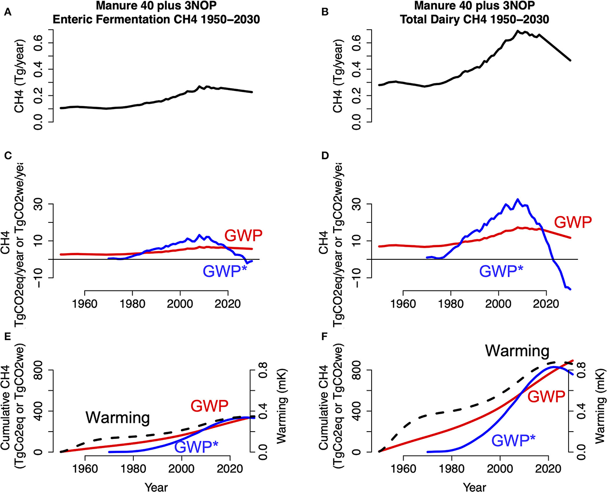
Figure 5. California future enteric fermentation and total “Manure 40 plus 3NOP” reduction scenario CH₄ emissions, comparison of these emissions converted to CO₂eq and CO₂we using GWP and GWP*, respectively, and cumulative CO₂eq and CO₂we with emissions-forced warming. The x-axis represents years, and the y-axis represents annual CH₄ emissions (A, B), annual CO₂eq or CO₂we (C, D), or cumulative CO₂eq or CO₂we (E, F). Enteric fermentation estimates are given by (A, C, E), and total dairy emissions are given by (B, D, F). CO₂we are represented in (C–F) by the blue solid line (“GWP*), CO₂eq are represented in (C–F) by the red solid line (“GWP”), and temperature is given in (E, F) by the dashed black line (“Warming”). The temperature axis (C) is scaled by 0.001 mK/TgCO₂, or 1 K/TtCO₂, as in previous figures. The horizontal black line in (C, D) is at y = 0.

Again, when each annual CO₂we emissions estimate was added up to give cumulative emissions, because some annual emissions rates were negative, cumulative CO₂we decreased from 2017 to 2030 (Figures 5E, F). In contrast, GWP-based cumulative CO₂eq continued to increase under declining future annual CH₄ emissions (Figures 5C, D). Warming forced by declining annual CH₄ emissions also declined, so cumulative GWP^*-based CO₂we reflected these dynamics better than cumulative GWP-based CO₂eq. Because the rate of decline of emissions is greatest in this scenario, the difference between GWP- and GWP^*-based emissions estimates and their agreement with warming dynamics is most clear in this scenario.

3.6. Relationship between cumulative CO₂eq and CO₂we from all scenarios and modeled warming

Figure 6 plots cumulative CO₂eq and CO₂we from historical, BAU, and reductions scenarios, respectively, against modeled warming. This plot shows the same information as previous plots, but allows us to directly visualize the relationship between cumulative CO₂ emissions and temperature change in this study. We expect cumulative CO₂ or CO₂-equivalent emissions and temperature to be linearly related, as this is a well-established physical relationship. In the historical period, annual background CH₄ emissions increased over time, and so both cumulative GWP-based CO₂eq and GWP^*-based CO₂we increased, as discussed in Section 3.2. Modeled temperature also increased over time in the historical periods, as expected given the linear relationship between cumulative CO₂ emissions and temperature change (Figure 6A).

FIGURE 6

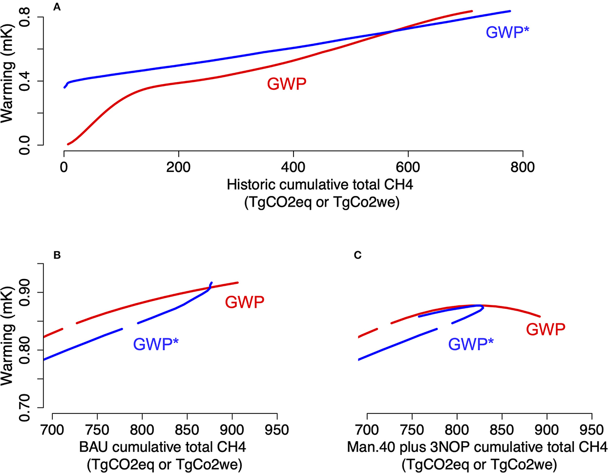
Figure 6. The relationship of CO₂eq and CO₂we with modeled warming response to these emissions. The x-axis shows cumulative CO₂eq calculated using GWP in red (“GWP”), or CO₂we calculated using GWP* in blue (“GWP*”). The y axis shows warming from annual CH₄. (A) Shows data from the historical (1950–2017) period. The slope of the line of cumulative CO₂ emissions and temperature change is approximately TCRE. (B) Shows future (2018–2029) BAU emissions, while (C) shows future (2018–2030) “Manure 40 plus 3NOP” reduction scenario emissions. Lines are broken between historical and future data.

Under the “Manure 40 plus 3NOP” future reductions scenario, annual background CH₄ emissions decrease over time. As discussed in Section 3.5, in this scenario, cumulative CO₂eq continue to increase in this scenario while cumulative CO₂we increased until 2017, then decreased. Temperature change forced by the background CH₄ emissions also increased until 2017, then decreased. That cumulative CO₂eq continue to increase implies that increasing cumulative emissions can cause decrease warming, which is an unphysical relationship (Figure 6B). In contrast, the relationship between cumulative CO₂we and warming is always linear—when cumulative CO₂we increase, warming is also increasing, but when CO₂we begin to decrease, warming also decreases and the blue line “turns back” on itself. This plot thus gives another visualization of results from previous plots, which are that CO₂we matched the dynamics of warming from declining background CH₄ emissions better than GWP-based emissions, or in other words can capture the physical relationship linking cumulative CO₂ emissions and temperature change that GWP does not.

In the manure and enteric CH₄ BAU scenario, annual background CH₄ emissions are approximately constant, as discussed in Section 3.3. Warming forced by these emissions “flatten out” during the period of constant background emissions. In this scenario, cumulative CO₂we “flatten out” and stop accumulating, while cumulative CO₂eq continue to increase. When cumulative CO₂eq are plotted against temperature change, while warming stays approximately constant, cumulative emissions continue to increase, implying that constant cumulative emissions can cause constant warming, which is an unphysical relationship (Figure 6B). In contrast, cumulative CO₂we stop increasing under these near-constant background emissions, almost “turning back” like in Panel C and again showing that GWP^*-based emissions dynamics match warming dynamics better under constant background emissions.

3.7. Husbandry factors driving declining California dairy CH₄ emissions from 2008 to 2017

Given the importance of capturing CH₄'s flow nature especially under declining emissions rates, we conducted a separate analysis from the hypothetical scenarios, including hypothetical reductions scenarios, giving the results described in Sections 3.1–3.6. We conducted this separate analysis to determine if California dairy background CH₄ emissions are in fact declining and, if so, to identify husbandry factors driving the decline in emissions. Historical annual CH₄ emissions decrease from 2008 to 2017 after a peak in 2008 (Figures 7A, B). This decrease in CH₄ emissions is likely a result of decreasing California dairy cattle populations, which peaked in 2009 (Figures 7A, C). Because CH₄ emissions depend heavily on cattle population, this decreasing population from 2009 to 2019 is likely driving decreasing CH₄ emissions. This decreasing cattle population in turn may be driven by increasing per capita milk production (Figure 7C), as per capita milk production has increased from 2009 to 2019 and per capita milk production and dairy population are negatively correlated from 2009 to 2019 (data not shown). Manure management CH₄ emissions have also been reduced by CDFA Dairy Digester Research and Development Program (DDRDP) since 2015 and Alternate Manure Management Program (AMMP) since 2017. The majority of reductions are due to DDRDP. These programs provide estimates of annual CH₄ reductions due to program implementation, which have been added to historical annual CH₄ emissions to plot putative emissions without these programs. Decreases in total CH₄ since 2008 have been driven by decreasing population and decreased CH₄ from manure management due to CDFA programs (Figure 7B).

FIGURE 7

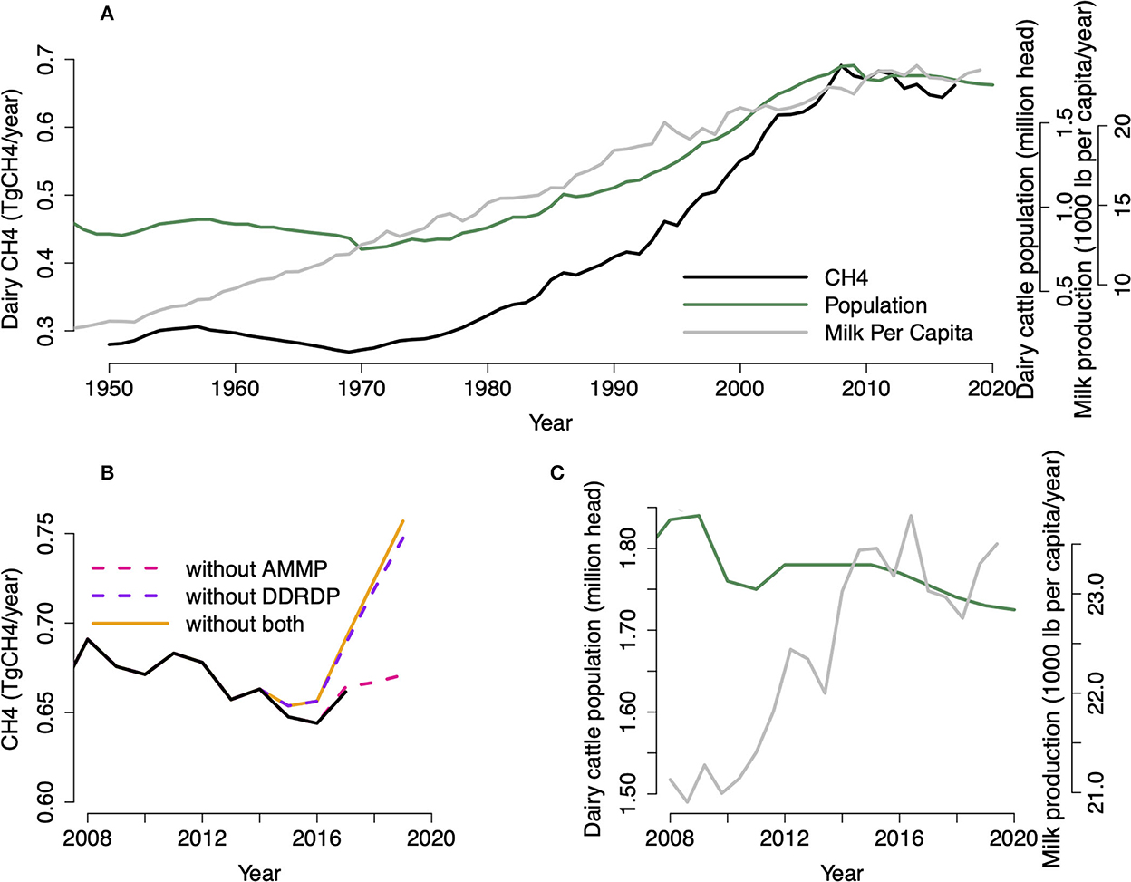
Figure 7. Mechanisms of decreasing CH₄ emissions since 2008 include decreasing dairy herd size, increasing per capita production, and manure management CH₄ reductions programs. In (A–C), the x-axis shows years; in (A) the entire historical time series is shown (1950–2017), while in (B, C), only 2008–2017 are shown. In (A, B), the y-axis is annual total dairy CH₄ emissions, but in (B) the y-axis does not begin at zero in order to provide a close-up view of CH₄ dynamics from 2008 to 2017. In (A), the right y axis shows per capita milk production and cattle population. (B) Shows hypothetical estimates of annual CH₄ reductions due to DDRDP and AMMP program implementation, which has been added to historical CH₄ emissions to plot putative emissions without these programs. The y-axis of (C) shows cattle population and the right y axis shows per capita milk production.

4. Discussion

4.1. Application of GWP^* to CH₄ emissions from livestock agriculture

Previous studies have applied GWP^* to large, RCP-based CH₄ datasets (Cain et al., 2019; Lynch et al., 2020). Ours builds upon this work and is the first to our knowledge to apply GWP^* to sectoral emissions from a North American animal production system, and thus serves as case study for the application of GWP^* to smaller industry- and locale-specific CH₄ emissions data. Previous authors have debated GWP^*'s applicability to sectoral and national emissions, which will be discussed further here. Nonetheless, previous authors have applied GWP^* and other alternative GHG metrics to local agricultural sectors, including Australian beef feedlots (Ridoutt et al., 2022), Australian sheep meat production (Ridoutt, 2021a), Australian livestock production (Ridoutt, 2021b), and Austrian dairy production (Hörtenhuber et al., 2022). Similar to reductions scenarios in our study, Ridoutt and coauthors found larger potential GHG reduction benefits from supplementing Australian beef steers with enteric CH₄-inhibiting macroalgae Asparagopsis taxiformis when emissions were assessed using GWP^* rather than GWP (Ridoutt et al., 2022). Similarly to our study, Hörtenhuber and coauthors found that decreasing lactating dairy cattle population due to improved production efficiency resulted in strong sectoral emission reductions from dairy production, which were greater when assessed with GWP^* than with GWP₁₀₀ (Hörtenhuber et al., 2022). In Australian livestock industries where CH₄ emissions increased from 1990 to 2018 (beef, pork, and dairy production), emissions from the beef cattle, pig meat and milk production industries assessed using GWP^* contributed to climate warming less than when assessed with the GWP₁₀₀ climate metric (Ridoutt, 2021b). While increasing background emissions in Australia from 1990 to 2018 are similar to our “historical” scenario, we found that under increasing background emissions, GWP^*-based emissions estimates were greater than those given by GWP. This discrepancy may be because the authors used total GHG emissions, not only CH₄, in their analysis. It may also result from annual Australian CH₄ emissions increasing by less than needed for CO₂we to exceed CO₂eq, 1% per year. In this study, dairy CH₄ emissions were 214 kt in 1990 and 275 kt in 2018, which gives an approximate rate of increase of 1% per year. Beef CH₄ emissions were 1,252 kt in 1990 and 1,421 in 2018, which gives an approximate rate of increase of 0.4% per year, below the approximate threshold for CO₂we greater than CO₂eq, discussed further immediately below.

4.2. Rate of change of CH₄ emissions leading to zero CO₂we emissions

Because of how the metrics are constructed, under a positive rate of change, CO₂we are greater than GWP-based CO₂-equivalent emissions when the rate of change of emissions is >1% per year. In our historical CH₄ emissions dataset, annual CH₄ emissions increased over time, leading to continuously increasing CO₂we. CO₂we are weighted heavily under increasing annual CH₄ emissions because CH₄ is being added to the atmosphere and CH₄ has a stronger radiative forcing per unit mass than CO₂ (Fuglestvedt et al., 2003). When CO₂eq are set equal to CO₂we (Equations 5 and 6), we see that $\frac{d{E}_i}{dt}$ is equal to E_i when $\frac{d{E}_i}{dt}$ = 0.01 × E_i. Thus, CO₂we will exceed CO₂eq when the rate of change of emissions is >1% per year, as noted by Lynch et al. (2020). The difference between CO₂eq and CO₂we suggests that GWP may underestimate, or that GWP^* may overestimate, the relative strength of CH₄ to CO₂ under increasing annual CH₄ emissions in the near term after a pulse emission, and that GWP may overestimate them in the long term, as was also found in studies using idealized (e.g., hypothetical, as opposed to historical) CH₄ emissions (Lynch et al., 2020).

Because CH₄ is a flow pollutant, under constant annual CH₄ emissions the rate of generation and removal of CH₄ are approximately equal over the atmospheric lifetime of CH₄ and there is no net accumulation of CH₄. To demonstrate that GWP^* can capture this short-lived behavior, Lynch et al. (2020) simulated a step increase to a sustained emission of CH₄, and found that over the first 20 years, CO₂we given by GWP^* exceeded emissions given by conventional GWP. After the first 20 years, however, the rate of change of CH₄ emissions is 0, and the only CH₄ emissions are those represented by the “stock” or s term (Cain et al., 2019). At the same time, GWP-derived emissions remain above zero with constant annual CH₄ emissions which represents the behavior of a stock gas like CO₂. Similarly, in our BAU scenario under approximately constant annual CH₄ emissions, CO₂eq remain constant, while CO₂we fall almost to zero except for the contribution of the stock term (Figure 3).

4.3. Linking cumulative CO₂we with temperature change

Under decreasing annual CH₄ emissions rates, more CH₄ will have been removed from the atmosphere than is produced to replace it, and negative annual CO₂we emissions suggest negative warming relative to the reference year in our study. Annual CO₂eq under decreasing annual CH₄ emissions, however, were never negative in our study or in that of Lynch et al. (2020).

In the present study, cumulative (annual emissions summed over time) CO₂we dynamics over time match those of warming, which also decrease under decreasing annual CH₄ emissions. Lynch et al. (2020) found that under declining CH₄ emissions, CO₂we were negative, and the temperature effect forced by these declining CH₄ emissions was less positive, like turning down a thermostat (note that any positive CH₄ emissions are still very strong warmers of the climate). In contrast, under declining annual CH₄ emissions, CO₂eq continued to accumulate, and GWP did not indicate the correct direction of temperature change. Thus, warming profiles confirm that GWP^*-based cumulative CO₂-warming equivalent emissions are able to represent the warming effects of CH₄ on the climate. Zhang et al. (2018) found that under declining SLCP emissions in the RCP 42.6 and 4.5 emission scenarios, effective radiative forcing from SLCP was negative. Cain et al. (2019) and Lynch et al. (2020) concluded that GWP^* captures the fundamentally different behavior of short- vs. long-lived climate pollutants, especially under declining CH₄ emissions, and therefore provides a reliable metric to directly link greenhouse gas emissions to warming.

Due to their linear relationship, cumulative CO₂ emissions can be linked to global temperature change with a coefficient known as the Transient Climate Response to Cumulative Carbon Emissions (TCRE). Cumulative CO₂we should result in global temperature change when multiplied by this constant, and this constant is approximately the slope of a line when cumulative emissions and warming are plotted against each other. Given the similar dynamics of warming and cumulative emissions over time, cumulative emissions could simply be multiplied by a constant, which was ~0.001 mK/Tg CO₂, or 1 K/Tt CO₂, to give temperature change. GWP-based estimates, however, could not be linked to temperature changed simply using a coefficient because cumulative CO₂eq had different dynamics over time than warming. Like Cain et al. (2019) we also found that GWP^*-based estimates plotted against temperature change resulted in a straight line, while GWP-based estimates did not. We found this line had an approximate slope of 1 K/Tt CO₂. The approximate change in temperature per unit cumulative CO₂ emissions that we found, 1 K/Tt CO₂, exceeds the IPCC likely range, possibly due to a large increase in annual CH₄ emissions in the 1950s leading to a larger GWP of CH₄ in this time period (Reisinger et al., 2011). The largest discrepancy between the dynamics of GWP^*-based estimates and warming is during the period from 1950 to 1980, where a “bulge” occurred, possibly due to this increased GWP of CH₄.

Using Equation 6 and setting CO₂we to zero, Cain et al. (2019), found the rate of CH₄ emission that is equivalent to zero CO₂we and thus to approximately stable temperatures over the time period Δt. With r = 0.75, s = 0.25, and H = 100 years, as used in the present study (following Cain et al., 2019), 0.3% is the rate of decline of CH₄ emissions (ΔE/Δt) under which CH₄-induced warming is stable. Under the “Manure 40 plus 3NOP” reduction scenario in the present study, the annual rate of decline of total CH₄ emissions from 2017 to 2030 is about 1.15%, while under “Manure 40 plus BAU EF,” the rate of decline of total CH₄ emissions is about 0.92%. Thus, under future SB 1383-mandated emissions reductions, California dairy CH₄ emissions will warm the climate less than they do without these reductions, even under scenarios that limit manure management CH₄ emissions reductions only. The rate of decline of historical CH₄ emissions from the peak in 2008 to 2017, was 3.26%, a decline which we suggest has been driven by declining California dairy herd size driven by increasing per capita milk production, as well as by the CDFA DDRDP after its introduction in 2015, with a minor contribution from AMMP. Thus, under their current and predicted rates of reduction, California dairy CH₄ emissions will be below the level at which stable warming effect will be actuated by these emissions and will reduce warming vs. 20 years ago. This behavior contrasts with CO₂, whose atmospheric concentrations and radiative forcing increase even under decreased emissions rates.

4.4. Contribution of SLCP to California emissions and applicability of GWP^* to emissions inventories

Mitigating SLCP emissions from dairy production centers on reducing CH₄ emissions from dairy manure management and reducing CH₄ from enteric fermentation. California has the largest dairy herd in the United States and thus the highest total (enteric fermentation plus manure management) dairy CH₄ emissions. California milk production feed efficiency is relatively high, making enteric fermentation emissions per unit California milk product relatively low (Naranjo et al., 2020). However, CH₄ emissions from cows in California are relatively higher on a per-dairy basis than those in the rest of the United States herd because flush water lagoon systems are the predominate manure management system in California dairies (CARB, 2022b), and anaerobic lagoons emit the most CH₄ per head of all common manure management practices (Owen and Silver, 2015). In 2017, agricultural manure management was California's second largest source of CH₄. Thus, preventing anaerobic conditions during manure management or capturing transforming CH₄ that is produced in anaerobic conditions represent major opportunities to reduce CH₄ from manure management (Montes et al., 2013). The CDFA Dairy Digester Research and Development Program (DDRDP) provides grants to finance the installation of dairy digesters, which capture CH₄ and convert it into fuel (CDFA, 2022b). CDFA's Alternative Manure Management Program (AMMP) provides grants to finance implementation of non-digester manure management practices in order to manage less manure anaerobically, such as solid separation or conversion from flushing to scraping or pasture-based management (CDFA, 2022a). Thus, CDFA's manure management CH₄ emissions reductions programs encompass both major targets for reductions. We have shown in this study that CDFA's programs, especially DDRDP, have successfully mitigated CH₄ emissions and have contributed to the decreasing CH₄ emissions rate in California since 2008.

In 2017, enteric fermentation was California's largest source of methane. Mitigation strategies for enteric fermentation center on use of feed additives such as rumen archaea inhibitors, ionophore antibiotics, or electron acceptors like nitrates (Hristov et al., 2014), and improved feed digestibility, which is unlikely to yield significant benefits in intensive production systems like California that already have relatively high feed efficiency (Herrero et al., 2016). 3NOP inhibits the methane-forming step in the rumen and is a promising feed additive, but production of 3NOP also emits GHG, decreasing net potential reductions (Feng and Kebreab, 2020). In this study, we evaluated reductions scenarios that included enteric fermentation CH₄ reduction, using maximum net potential 3NOP reductions. For our manure management reduction scenarios, we used 40% reduction of 2013 levels as mandated by SB 1383 without evaluating the feasibility of these reductions and assumed 40% represented net reductions. For this reason, enteric fermentation's relatively smaller impact on emissions reductions in our scenarios is not necessarily representative of its true impact relative to manure management mitigation programs. Indeed, over the past 50 years in California, reductions in CH₄ from enteric fermentation have been about five times greater than reductions in CH₄ from manure management (Naranjo et al., 2020). However, because California SB 1383 does not require any specific enteric fermentation reductions, we used potential net 3NOP reductions, while we assumed that 40% manure management methane reductions were feasible because they are mandated by SB 1383. Nonetheless, our study demonstrated that GWP^* can accurately represent the warming effects of CO₂eq under potential enteric fermentation CH₄ reductions and thus can serve as an important tool of evaluating on-farm CH₄ mitigation strategies in the future.

We used 2017 enteric fermentation emission factors to calculate emissions from dairy cows from 2017 to 2029 under the “business-as-usual” scenario, assuming that enteric fermentation emissions factors would be stable from 2017 to 2029. However, the true dynamics of future enteric fermentation emissions factors may be more complex. Enteric CH₄ emissions factors for California dairy cattle remained constant from 2012 to 2020 (CARB, 2022a). In contrast, U.S.-wide emissions factors increased by 8.7% from 2010 to 2020 (EPA, 2022). The relative stability of California dairy enteric CH₄ emissions factors may reflect interplay between increasing milk production and improvements in feed efficiency. Increased per capita milk production could associated with greater feed intake and thus increasing enteric CH₄ emissions factors, as both CARB and EPA develop enteric CH₄ emissions factors CH₄ conversion rate, which is the fraction of gross energy (GE) in feed converted to CH₄, and GE intake increases with increasing net energy for lactation (NE_L), which itself increases with increasing milk production (IPCC, 2006; CARB, 2022a; EPA, 2022). However, a life cycle analysis comparing California dairy environmental footprints in 1964 and 2014 found that in 1964, the feed conversion rate was 1.93 kg feed per kg energy-corrected milk (ECM), while in 2014, the feed conversion ratio was 0.79–0.81 kg of feed/kg of ECM, suggesting cattle today utilize feed more efficiently than those 50 years ago. In 1964, each cow emitted 0.98 kg of CO₂ equivalents of enteric methane per kg ECM compared with 0.43–0.45 kg of CO₂ equivalents of enteric methane per kg ECM in 2014 (Naranjo et al., 2020). Average ECM production in 1964 was 15.73 kg/day, while it was 39.8 kg/day in 2014, making enteric methane emissions factors 15.4 kg CO₂ equivalents per day in 1964 and 17.11–17.9 kg CO₂ equivalents per day in 2014.

Previous authors have predicted future inventories of livestock methane emissions assuming constant or even decreasing CH₄ emissions intensities (emissions per unit product, where product is kg of protein in this case) (Chang et al., 2021). Chang et al. projected livestock methane emissions out to 2050 using different pathways of assumed emission intensity changes. These authors used two pathways with contrasting assumptions about production efficiency changes: constant emission intensity and improving efficiency (i.e., decreasing emission intensity). The “constant intensity” pathway assumed that no changes in methane emission intensities would take place in the future. The “improving efficiency” pathway was based on decreasing trends in emission intensity during the past two decades due to increasing production efficiency. Based on this finding, they constructed a “improving efficiency” pathway, assuming continuing decreases in emission intensity. Under this pathway, emissions intensities in countries showing decreasing emission intensity during the past two decades followed this decreasing trend into the future, while a constant emission intensity was applied for countries that experienced no change or an increasing emission intensity in the past two decades. Thus, other studies in the field have found it reasonable to assume constant emissions intensity of livestock products into the future. The assumption that increasing production efficiency will lead to constant or decreasing emissions intensities is not necessarily the same as the assumption that increasing production efficiency will lead to constant emissions factors, because increasing production could still lead to increasing total (e.g., not on a per-product basis) emissions. However, enteric CH₄ emissions factors for California dairy cattle given by CARB remained constant from 2012 to 2020. Over this time, California milk production was as follows: 23,457 lbs. per head in 2012; 23,178 lbs. per head in 2013; 23,786 lbs. per head in 2014; 23,028 in 2015; 22,968 in 2016; 22,755 in 2017; 23,301 in 2018; 23,533 in 2019; and 23,990 in 2020 (USDA National Agricultural Statistics Service, 2022). Annual change in milk production, averaged over these 8 years, is 0.26%. Thus, if milk production was approximately constant, and milk emissions intensity was approximately constant or decreasing, then enteric CH₄ per cow (e.g., enteric CH₄ emissions factor) could remain approximately constant.

Because CH₄ emissions factors are estimated based on dietary and production parameters, if regionally typical diets and production remain approximately the same over time, emissions factors will remain the same from year to year. CARB likely has assumed that the diets of California dairy cattle have remained approximately constant, given that the emissions factors they have calculated remain constant from 2012 to 2020. Thus, several lines of evidence underscore that it is a reasonable assumption that enteric fermentation factors will remain approximately constant to 2029 in the BAU scenario. However, this trend does not necessarily apply to other states and production situations, and enteric fermentation emissions factors may be more variable than assumed in our study. In the BAU scenario, this assumption led to approximately constant annual CH₄ emissions, and thus declining GWP^* emissions over time. Had enteric CH₄ emissions factors continued to rise over time, the dynamics of the scenario would be similar to the historic (1950–2017) scenario, in which enteric CH₄ emissions factors and annual CH₄ emissions did increase over time. The purpose of our “BAU” scenario was to investigate GWP^* dynamics relative to GWP dynamics given approximately constant annual CH₄ emissions. The “BAU” scenario utilized projected dairy cattle population data to estimate future populations under typical policy and macroeconomic conditions and projected a 0.32% decrease in population from 2018 to 2029. This small decrease in population over time, along with the constant enteric fermentation and manure management CH₄ emissions factors used, gives approximately constant annual CH₄ emissions and provides a scenario to investigate the difference in dynamics between GWP- and GWP^*-based estimates under constant background CH₄ emissions, unlike the historical (increasing background emissions) or reductions (decreasing background emissions) scenarios. Thus, while further investigation on trends in enteric fermentation and manure management emissions factors and future dairy cattle populations is needed, the assumption of constant California CH₄ emissions factors from 2017 to 2029 is in line with CARB emissions factors and sufficient for our study's purposes.

The goal of California's annual GHG emission inventory is to establish historical emission trends and track sectoral progress in achieving statewide reductions goals. The 2021 edition of the inventory and previous iterations provide emissions estimates in CO₂eq using GWP₁₀₀ values from IPCC AR4, consistent with current international and national GHG inventory practices (CARB, 2022a). In addition, SB 1383 mandates reductions in annual emissions rates, not warming effects, of dairy manure CH₄ by 2030. Thus, because goals are centered on emissions reductions, not warming impacts, GWP may still be an appropriate metric for these purposes. However, attribution of the warming impacts of the economic sectors whose emissions are quantified in emissions inventories requires a metric that can capture the dynamics of cumulative SLCP emissions over time, such as GWP^*. GWP^* and GWP could coexist given the different policy goals of economic sectors or state or local governments, as recommended by the IPCC AR6 Working Party I report.

4.5. Limitations of GWP^*

Notwithstanding GWP^*'s improved representation of CH₄'s flow gas-nature, any single-number metric may result in oversimplification of complex climate dynamics and underestimation of the warming response to SLCP emissions (Collins et al., 2020). Some arbitrary decisions still underlie GWP^*, such as the time horizon H, or the designation of a certain climate pollutant as “short-lived” and thus the employment of GWP^*, which depends on the time scale being considered (Lynch et al., 2020). While the calculation of GWP^* is subject to some arbitrary decisions, the concept of CO₂eq is not necessarily physically accurate. Climate responses to CO₂ and CH₄ are both temperature- and scenario-dependent, so different emissions scenarios with identical CO₂eq can have vastly different impacts on global temperature. For this reason, no single scaling factor can truly convert between CO₂ and CH₄ emissions across all scenarios (Fuglestvedt et al., 2000).

Previous authors have suggested that because it is based on past emissions, GWP^* unfairly and unethically penalizes developing countries when applied at sub-global levels (Rogelj and Schleussner, 2019). Rogelj and Schleussner argue that due to GWP^*'s “grandfathering” effect, countries with high historic SLCP emissions are rewarded because reductions from these emissions lead to declining cumulative CO₂we, while countries with historically low SLCP emissions (i.e., typically developing countries) are penalized for increasing emissions which may result from socioeconomic development. While not stated in this critique, presumably similar limitations apply to emissions from specific economic sectors. In their response, Cain et al. (2021) note that this “unintentional unfairness” would result from any warming-equivalent-based metric that differentiates the behavior of stock and flow pollutants, such as combined global temperature change potential (CGTP) (Collins et al., 2020). Furthermore, because IPCC AR6 does not recommend any given emission metric, metric appropriateness depends on given policy goals. Cain et al. (2021) argue that in policy contexts with long-term temperature goals as the Paris Agreement, GWP^* is useful because it demonstrates that the relationship between a country's CH₄ emissions and temperature change scales with current CH₄ emissions plus a contribution from past CH₄ emissions, which conventional GWP cannot. They argue that quantifying this relationship is not itself necessarily unfair or unequitable, given that quantification of historical contributions of a country's SLCP to warming using GWP^* and taking these contributions into burden-sharing policy are separate, and the latter are determined by policy-makers, although using a metric that reflects the impact of all gases on temperature change would facilitate such policy discussions (Cain et al., 2021).

In spite of potential limitations of the CO₂ equivalence concept and GWP^*, CO₂-equivalence-based climate metrics remain a prevalent policy tool (UNFCCC, 2020). GWP^* provides an accessible and temperature goal-relevant adjustment of current CO₂-equivalence methodology that does not require any additional information from what is already typically reported. Other metrics that have been proposed as alternatives to GWP, such as Global Temperature Change Potential (GTP), combined GWP, or CGTP, require additional inputs that are themselves dependent on uncertainties in the climate system and future emissions scenarios (Shine et al., 2007; Collins et al., 2020). GWP^* has been shown to underestimate the contribution of CH₄ to temperature change by up to 20% compared to CGTP, which employs a more explicit calculation of the effect of CH₄ emissions rate change relative to a pulse emission of CO₂ (Collins et al., 2020). However, Collins et al. (2020) also note that the more complex emissions metrics CGWP or GTP are structurally similar to GWP^* and provide only changes in precise values, not conceptual foundation or development, whereas using the conventional GWP is unable to represent the correct sign of warming from decreasing SLCP emissions, as we have shown. While Wigley (1998) argues that unlike the GWP framework, emissions equivalence should be based on radiative-forcing based Forcing Equivalence Index (FEI), other authors consider both GWP and GWP^* reasonable approximations to FEI (Enting and Clisby, 2021).

5. Conclusions

We have used California dairy production as a case study for the application of the novel GHG metric GWP^*, following its recent development and publication. While recent publications have shown the applicability of GWP^* to global emissions datasets spanning all SLCP emissions sectors, we have applied GWP^* to a California dairy CH₄ emissions inventory and discussed the applicability of GWP^* to local and single-sector inventories, which some authors argue is limited. GWP^* provides a direct relationship between cumulative emissions and their warming effects, which conventional GWP does not. This relationship exists because GWP^* represents methane's short-lived nature, by which it does not accumulate in the atmosphere under declining emissions, unlike CO₂. We found that conventional GWP underrepresents the warming impacts of dairy CH₄ emissions in CA under increasing emissions rates, and overrepresents their warming impacts under declining emissions rates. GWP^* represents that under declining emissions rates, cumulative California dairy CH₄ decrease and warming forced by these emissions also decreases, although any CH₄ that continues to be emitted is still a strong climate forcer. In contrast, under declining annual CH₄ emissions, GWP-based CO₂-equivalent emissions (CO₂eq) continued to accumulate, so GWP did not indicate the correct direction of temperature change. While IPCC AR6 makes clear that metric choice depends on policy goals, given its ability to unambiguously link warming impacts to SLCP emissions, GWP^* may provide a more accurate tool for quantifying SLCP emissions into policy contexts that specifically aim to limit global warming, such as the Paris Agreement.

Data availability statement

The raw data supporting the conclusions of this article will be made available by the authors, without undue reservation.

Author contributions

EP designed the research approach, compiled data, wrote the R code to analyze the results, analyzed the results, and prepared the manuscript. SL helped design the research approach and provided data and support in carrying out the research. FM proposed the research question and supervised the work. All authors reviewed drafts of the manuscript, provided feedback, and approved the final version.

Funding

Financial support to EP was provided by the Students Training in Advanced Research (STAR) Program at the UC Davis School of Veterinary Medicine through the Ritchie Hill endowment funds, SAVMA AWESC Environmental Awareness Grant, and NIH Grant T32GM136559.

Acknowledgments

We gratefully acknowledge Joe Proudman for his helpful feedback. We acknowledge researchers at FAPRI and AMAP for providing information about the methodology used in FAPRI/AMAP projections.

Conflict of interest

The authors declare that the research was conducted in the absence of any commercial or financial relationships that could be construed as a potential conflict of interest.

Publisher's note

All claims expressed in this article are solely those of the authors and do not necessarily represent those of their affiliated organizations, or those of the publisher, the editors and the reviewers. Any product that may be evaluated in this article, or claim that may be made by its manufacturer, is not guaranteed or endorsed by the publisher.

Supplementary material

The Supplementary Material for this article can be found online at: https://www.frontiersin.org/articles/10.3389/fsufs.2022.1072805/full#supplementary-material

Abbreviations

E_CH4, total annual CH₄ emissions (kg CH₄ per year); E_EF, annual enteric fermentation CH₄ emissions (kg CH₄ per year); E_MM, annual manure management CH₄ emissions (kg CH₄ per year); 3NOP, 3-nitrooxypropanol; AMMP, Alternative Manure Management Program; BAU, Business-as-usual; BAU EF, “business as usual” enteric fermentation scenario; CH₄, Methane; CO₂, carbon dioxide; CO₂eq, CO₂-equivalent emissions; CO₂we, CO₂-warming equivalent emissions; DDRDP, dairy digester research and development program; GHG, greenhouse gas; GWP, global warming potential; GWP^*, global warming potential star; Man 40 plus BAU EF, manure management 40% reduction scenario added to the “business as usual” enteric fermentation (BAU EF) scenario; MMP, manure management practice; Pop_dairy, annual dairy cow population (head dairy cow); r, weight assigned to the rate-dependent warming effects of given SLCP in GWP^*; RF_i, radiative forcing; s, weight assigned to the stock (long-term equilibration to past increases in forcing) contribution of given SLCP to GWP^*; SLCP, short-lived climate pollutant; TCRE, transient climate response to cumulative carbon emissions; Tg, Teragrams, equivalent to million metric tons (MMT).

References

Allen, M. R., Frame, D. J., Huntingford, C., Jones, C. D., Lowe, J. A., Meinshausen, M., et al. (2009). Warming caused by cumulative carbon emissions towards the trillionth tonne. Nature 458, 1163–1166. doi: 10.1038/nature08019

PubMed Abstract | CrossRef Full Text | Google Scholar

Allen, M. R., Shine, K. P., Fuglestvedt, J. S., Millar, R. J., Cain, M., Frame, D. J., et al. (2018). A solution to the misrepresentations of CO2-equivalent emissions of short-lived climate pollutants under ambitious mitigation. NPJ Clim. Atmos. Sci. 1, 1–8. doi: 10.1038/s41612-018-0026-8

CrossRef Full Text | Google Scholar

Blayney, D., and Normile, M. A. (2004). Economic Effects of U.S. Dairy Policy and Alternative Approaches to Milk Pricing: Report to Congress (Administrative Publication Number 076). Washington, DC: USDA. Available online at: http://ageconsearch.umn.edu (accessed August 16, 2022).

Google Scholar

Bond, T. C., Doherty, S. J., Fahey, D. W., Forster, P. M., Berntsen, T., DeAngelo, B. J., et al. (2013). Bounding the role of black carbon in the climate system: a scientific assessment. J. Geophys. Res. Atmos. 118, 5380–5552. doi: 10.1002/jgrd.50171

CrossRef Full Text | Google Scholar

Cain, M., Lynch, J., Allen, M. R., Fuglestvedt, J. S., Frame, D. J., and Macey, A. H. (2019). Improved calculation of warming-equivalent emissions for short-lived climate pollutants. NPJ Clim. Atmos. Sci. 2, 4. doi: 10.1038/s41612-019-0086-4

PubMed Abstract | CrossRef Full Text | Google Scholar

Cain, M., Shine, K., Frame, D., Lynch, J., Macey, A., Pierrehumbert, R., et al. (2021). Comment on “Unintentional unfairness when applying new greenhouse gas emissions metrics at country level”. Environ. Res. Lett. 16, 68001. doi: 10.1088/1748-9326/ac02eb

CrossRef Full Text | Google Scholar

Capper, J. L., Cady, R. A., and Bauman, D. E. (2009). The environmental impact of dairy production: 1944 compared with 2007. J. Anim. Sci. 87, 2160–2167. doi: 10.2527/jas.2009-1781

PubMed Abstract | CrossRef Full Text | Google Scholar

CARB (2022a). 3A1ai—Livestock—Enteric Fermentation—Cattle—Dairy Cows Year 2019, Documentation of California's Greenhouse Gas Inventory. Sacramento, CA: CARB. Available online at: https://ww2.arb.ca.gov/sites/default/files/ghg-inventory-doc/newdoc/docs3/3a1ai_entericfermentation_livestockpopulation_dairycows_ch4_2019.htm (accessed August 12, 2022).

Google Scholar

CARB (2022b). 3A2ai—Livestock—Manure Management—Cattle—Dairy Cows Year 2019, Documentation of California's Greenhouse Gas Inventory. Sacramento, CA: CARB. Available online at: https://ww2.arb.ca.gov/applications/california-ghg-inventory-documentation (accessed August 12, 2022).

CARB (2022c). Analysis of Progress Toward Achieving the 2030 Dairy and Livestock Sector Methane Emissions Target. Sacramento, CA: CARB. Available online at: https://ww2.arb.ca.gov/resources/documents/dairy-livestock-sb1383-analysis (accessed August 12, 2022).

CDFA (2000). California Agricultural Resource Directory 2000. Baltimore: CDFA.

CDFA (2007). California Agricultural Resource Directory 2006. Baltimore: CDFA.

Google Scholar

CDFA (2022a). Alternative Manure Management Program, Office of Environmental Farming and Innovation. Baltimore: CDFA. Available online at: https://www.cdfa.ca.gov/oefi/ammp/ (accessed August 12, 2022).

CDFA (2022b). Dairy Digester Research and Development Program, Office of Environmental Farming and Innovation. Baltimore: CDFA. Available online at: https://www.cdfa.ca.gov/oefi/ddrdp/ (accessed August 12, 2022).

Chang, J., Peng, S., Yin, Y., Ciais, P., Havlik, P., and Herrero, M. (2021). The key role of production efficiency changes in livestock methane emission mitigation. AGU Adv. 2, 391. doi: 10.1029/2021AV000391

CrossRef Full Text | Google Scholar

Collins, W. J., Frame, D. J., Fuglestvedt, J. S., and Shine, K. P. (2020). Stable climate metrics for emissions of short and long-lived species—combining steps and pulses. Environ. Res. Lett. 15, 024018. doi: 10.1088/1748-9326/ab6039

CrossRef Full Text | Google Scholar

Cui, T., Ding, Z., and Fu, X. (2017). Effects of straw and biochar addition on soil nitrogen, carbon, and super rice yield in cold waterlogged paddy soils of North China. J. Integ. Agric. 16, 1064–1074. doi: 10.1016/S2095-3119(16)61578-2

CrossRef Full Text | Google Scholar

den Elzen, M. G. J., and Lucas, P. L. (2005). The FAIR model: a tool to analyse environmental and costs implications of regimes of future commitments. Environ. Model. Assess. 10, 115–134. doi: 10.1007/s10666-005-4647-z

CrossRef Full Text | Google Scholar

Dijkstra, J., Bannink, A., France, J., Kebreab, E., and van Gastelen, S. (2018). Short communication: antimethanogenic effects of 3-nitrooxypropanol depend on supplementation dose, dietary fiber content, and cattle type. J. Dairy Sci. 101, 9041–9047. doi: 10.3168/jds.2018-14456

PubMed Abstract | CrossRef Full Text | Google Scholar

Duin, E. C., Wagner, T., Shima, S., Prakash, D., Cronin, B., Yáñez-Ruiz, D. R., Duval, S., Rümbeli, R., Stemmler, R. T., Thauer, R. K., and Kindermann, M. (2016). Mode of action uncovered for the specific reduction of methane emissions from ruminants by the small molecule 3-nitrooxypropanol. Proc. Natl. Acad. Sci. 113, 6172–6177. doi: 10.1073/pnas.1600298113

PubMed Abstract | CrossRef Full Text | Google Scholar

Enting, I., and Clisby, N. (2021). Technical note: On comparing greenhouse gas emission metrics. Atmos. Chem. Phys. 21, 4699–4708. doi: 10.5194/acp-21-4699-2021

CrossRef Full Text | Google Scholar

EPA (2013a). Inventory of U.S. Greenhouse Gas Emissions and Sinks: 1990–2011 U.S. Environmental Protection Agency. Annex 3.10: Methodology for Estimating CH4 Emissions from Enteric Fermentation. Washington, DC: EPA. Available online at: https://www.epa.gov/sites/default/files/2015-12/documents/us-ghg-inventory-2013-annexes.pdf (accessed August 10, 2022).

Google Scholar

EPA (2013b). Inventory of U.S. Greenhouse Gas Emissions and Sinks: 1990–2011 U.S. Environmental Protection Agency. Annex 3.11: Methodology for Estimating CH₄ and N₂O Emissions from Manure Management. Washington, DC: EPA. Available online at: https://www.epa.gov/sites/default/files/2015-12/documents/us-ghg-inventory-2013-annexes.pdf (accessed November 6, 2022).

Google Scholar

EPA (2022). Inventory of U.S. Greenhouse Gas Emissions and Sinks: 1990–2020 Annex 3.10. Washington, DC: EPA. Available online at: https://www.epa.gov/system/files/documents/2022-04/us-ghg-inventory-2022-annex-3-additional-source-or-sink-categories-part-a.pdf

Google Scholar

Fabiosa, J., Beghin, J., De Cara, S., Elobeid, A., Fang, C., Isik, M., et al. (2005). The doha round of the world trade organization and agricultural markets liberalization: impacts on developing economies. Rev. Agric. Econ. 27, 317–335. doi: 10.1111/j.1467-9353.2005.00252.x

CrossRef Full Text | Google Scholar

FAPRI AMAP (2020a). Baseline Review 2020: U.S. Livestock and Dairy Tables, University of Missouri. Washington, DC: FAPRI and AMAP. Available online at: https://www.fapri.missouri.edu/baseline-review-2020/ (accessed August 11, 2022).

Google Scholar

FAPRI AMAP (2020b). US Agricultural Market Outlook: Agricultural Markets and Policy Trade Friction Baseline and a Phase 1 Scenario (FAPRI-MU Report #01-20). Missouri: University of Missouri. Available online at: https://www.fapri.missouri.edu/publication/2020-u-s-agricultural-market-outlook/ (accessed August 12, 2022).

Google Scholar

Feng, X., and Kebreab, E. (2020). Net reductions in greenhouse gas emissions from feed additive use in California dairy cattle. PLoS ONE 15, e0234289. doi: 10.1371/journal.pone.0234289

PubMed Abstract | CrossRef Full Text | Google Scholar

Fuglestvedt, J. S., Berntsen, T. K., Godal, O., Sausen, R., Shine, K. P., and Skodvin, T. (2003). Metrics of climate change: assessing radiative forcing and emission indices. Clim. Change 58, 267–331. doi: 10.1023/A:1023905326842

CrossRef Full Text | Google Scholar

Fuglestvedt, J. S., Berntsen, T. K., Godal, O., and Skodvin, T. (2000). Climate implications of GWP-based reductions in greenhouse gas emissions. Geophys. Res. Lett. 27, 409–412. doi: 10.1029/1999GL010939

CrossRef Full Text | Google Scholar

Gulev, S. K., Thorne, P. W., Ahn, J., Dentener, F. J., Domingues, C. M., Gerland, S., et al. (2021). “Changing state of the climate system,” in Climate Change 2021: The Physical Science Basis. Contribution of Working Group I to the Sixth Assessment Report of the Intergovernmental Panel on Climate Change, eds V. Masson-Delmotte, P. Zhai, A. Pirani, S. L. Connors, C. Péan, S. Berger, et al. (Cambridge, New York, NY: Cambridge University Press).

Google Scholar

Herrero, M., Henderson, B., Havlík, P., Thornton, P. K., Conant, R. T., Smith, P., et al. (2016). Greenhouse gas mitigation potentials in the livestock sector. Nat. Clim. Change 6, 452–461. doi: 10.1038/nclimate2925

PubMed Abstract | CrossRef Full Text | Google Scholar

Hörtenhuber, S. J., Seiringer, M., Theurl, M. C., Größbacher, V., Piringer, G., Kral, I., et al. (2022). Implementing an appropriate metric for the assessment of greenhouse gas emissions from livestock production: a national case study. Animal 16, 100638. doi: 10.1016/j.animal.2022.100638

PubMed Abstract | CrossRef Full Text | Google Scholar

Hristov, A. N., Oh, J., Firkins, J. L., Dijkstra, J., Kebreab, E., Waghorn, G., et al. (2014). SPECIAL TOPICS: mitigation of methane and nitrous oxide emissions from animal operations: I. A review of enteric methane mitigation options 1. J. Anim. Sci. 91, 5045–5069. doi: 10.2527/jas.2013-6583

PubMed Abstract | CrossRef Full Text | Google Scholar

IPCC (2006). 2006 IPCC Guidelines for National Greenhouse Gas Inventories, Prepared by the National Greenhouse Gas Inventories Programme. Geneva: IPCC

Google Scholar

IPCC (2021). “Summary for policymakers,” in Climate Change 2021: The Physical Science Basis. Contribution of Working Group I to the Sixth Assessment Report of the Intergovernmental Panel on Climate Change, eds V. Masson-Delmotte, P. Zhai, A. Pirani, S.L. Connors, C. Péan, S. Berger, et al. (Cambridge: Cambridge University Press).

Google Scholar

Johnson, S. R., Meyers, W. H., Devadoss, S., Westhoff, P., Helmar, M. D., Skold, K. D., et al. (1993). “Policy Scenarios with the FAPRI Modeling System (No. 606),” in Agricultural Sector Models for the United States. Ames: Iowa State University Press.

Google Scholar

Kai, F. M., Tyler, S. C., Randerson, J. T., and Blake, D. R. (2011). Reduced methane growth rate explained by decreased Northern Hemisphere microbial sources. Nature 476, 194–197. doi: 10.1038/nature10259

PubMed Abstract | CrossRef Full Text | Google Scholar

Lamarque, J. F., Bond, T. C., Eyring, V., Granier, C., Heil, A., Klimont, Z., et al. (2010). Historical (1850–2000) gridded anthropogenic and biomass burning emissions of reactive gases and aerosols: methodology and application. Atmos. Chem. Phys. 10, 7017–7039. doi: 10.5194/acp-10-7017-2010

CrossRef Full Text | Google Scholar

Lara (2016). Senate Bill No. 1383 Chapter 395. New York, NY: California State Senate. Available online at: https://leginfo.legislature.ca.gov/faces/billTextClient.xhtml?bill_id=201520160SB1383 (accessed August 10, 2022).

Google Scholar

Lynch, J., Cain, M., Pierrehumbert, R., and Allen, M. (2020). Demonstrating GWP: a means of reporting warming-equivalent emissions that captures the contrasting impacts of short-A and long-lived climate pollutants. Environ. Res. Lett. 15, 44023. doi: 10.1088/1748-9326/ab6d7e

PubMed Abstract | CrossRef Full Text | Google Scholar

Matthews, H. D., Gillett, N. P., Stott, P. A., and Zickfeld, K. (2009). The proportionality of global warming to cumulative carbon emissions. Nature 459, 829–832. doi: 10.1038/nature08047

PubMed Abstract | CrossRef Full Text | Google Scholar

Millar, R. J., Nicholls, Z. R., Friedlingstein, P., and Allen, M. R. (2017). A modified impulse-response representation of the global near-surface air temperature and atmospheric concentration response to carbon dioxide emissions. Atmos. Chem. Phys. 17, 7213–7228. doi: 10.5194/acp-17-7213-2017

CrossRef Full Text | Google Scholar

Montes, F., Meinen, R., Dell, C., Rotz, A., Hristov, A. N., Oh, J., et al. (2013). SPECIAL TOPICS: Mitigation of methane and nitrous oxide emissions from animal operations: II. A review of manure management mitigation options. J. Anim. Sci. 91, 5070–5094. doi: 10.2527/jas.2013-6584

PubMed Abstract | CrossRef Full Text | Google Scholar

Myhre, G., Shindell, D., Bréon, F.-M., Collins, W., Fuglestvedt, J., Huang, J., et al. (2013). “Anthropogenic and natural radiative forcing,” in Climate Change 2013: The Physical Science Basis. Contribution of Working Group I to the Fifth Assessment Report of the Intergovernmental Panel on Climate Change, eds T. F. Stocker, D. Qin, G.-K. Plattner, M. Tignor, S. K. Allen, J. Boschung, A. Nauels, Y. Xia, V. Bex, and P. M. Midgley (Cambridge; New York, NY: Cambridge University Press), 659–740. Available online at: https://www.ipcc.ch/site/assets/uploads/2018/02/WG1AR5_Chapter08_FINAL.pdf

PubMed Abstract | Google Scholar

Naranjo, A., Johnson, A., Rossow, H., and Kebreab, E. (2020). Greenhouse gas, water, and land footprint per unit of production of the California dairy industry over 50 years. J. Dairy Sci. 103, 3760–3773. doi: 10.3168/jds.2019-16576

PubMed Abstract | CrossRef Full Text | Google Scholar

Nisbet, E. G., Manning, M. R., Dlugokencky, E. J., Fisher, R. E., and Lowry, D. (2016). Rising atmospheric methane: 2007–2014 growth and isotopic shift. Glob. Biogeochem. Cycles 30, 1356–1370. doi: 10.1002/2016GB005406

CrossRef Full Text | Google Scholar

Ocko, I. B., Sun, T., Shindell, D., Oppenheimer, M., Hristov, A. N., Pacala, S. W., et al. (2021). Acting rapidly to deploy readily available methane mitigation measures by sector can immediately slow global warming. Environ. Res. Lett. 16, 054042. doi: 10.1088/1748-9326/abf9c8

CrossRef Full Text | Google Scholar

Owen, J. J., and Silver, W. L. (2015). Greenhouse gas emissions from dairy manure management: a review of field-based studies. Glob. Change Biol. 21, 550–565. doi: 10.1111/gcb.12687

PubMed Abstract | CrossRef Full Text | Google Scholar

Persson, U. M., Johansson, D. J., Cederberg, C., Hedenus, F., and Bryngelsson, D. (2015). Climate metrics and the carbon footprint of livestock products: Where's the beef? Environ. Res. Lett. 10, 5. doi: 10.1088/1748-9326/10/3/034005

CrossRef Full Text | Google Scholar

Pierrehumbert, R. T. (2014). Short-lived climate pollution. Ann. Rev. Earth Planet. Sci. 42, 341–379. doi: 10.1146/annurev-earth-060313-054843

CrossRef Full Text | Google Scholar

R Core Team (2020). R: A Language and Environment for Statistical Computing. New York, NY: R Foundation for Statistical Computing. Available online at: https://www.r-project.org (accessed August 10, 2022).

Google Scholar

Reisinger, A., Havlik, P., Riahi, K., Van Vliet, O., Obersteiner, M., and Herrero, M. (2013). Implications of alternative metrics for global mitigation costs and greenhouse gas emissions from agriculture. Clim. Change 117, 677–690. doi: 10.1007/s10584-012-0593-3

CrossRef Full Text | Google Scholar

Reisinger, A., Meinshausen, M., and Manning, M. (2011). Future changes in global warming potentials under representative concentration pathways. Environ. Res. Lett. 6, 024020. doi: 10.1088/1748-9326/6/2/024020

CrossRef Full Text | Google Scholar

Ridoutt, B. (2021a). Climate neutral livestock production: a radiative forcing-based climate footprint approach. J. Clean. Prod. 291, 125260. doi: 10.1016/j.jclepro.2020.125260

CrossRef Full Text | Google Scholar

Ridoutt, B. (2021b). Short communication: climate impact of Australian livestock production assessed using the GWP^* climate metric. Livestock Sci. 246, 104459. doi: 10.1016/j.livsci.2021.104459

CrossRef Full Text | Google Scholar

Ridoutt, B., Lehnert, S. A., Denman, S., Charmley, E., Kinley, R., and Dominik, S. (2022). Potential GHG emission benefits of Asparagopsis taxiformis feed supplement in Australian beef cattle feedlots. J. Clean. Prod. 337, 130499. doi: 10.1016/j.jclepro.2022.130499

CrossRef Full Text | Google Scholar

Rogelj, J., and Schleussner, C.-F. (2019). Unintentional unfairness when applying new greenhouse gas emissions metrics at country level. Environ. Res. Lett. 14, 114039. doi: 10.1088/1748-9326/ab4928

CrossRef Full Text | Google Scholar

Schaefer, H., Fletcher, S. E. M., Veidt, C., Lassey, K. R., Brailsford, G. W., Bromley, T. M., et al. (2016). A 21st-century shift from fossil-fuel to biogenic methane emissions indicated by 13CH4. Science 352, 80–84. doi: 10.1126/science.aad2705

PubMed Abstract | CrossRef Full Text | Google Scholar

Schwietzke, S., Sherwood, O. A., Bruhwiler, L. M., Miller, J. B., Etiope, G., Dlugokencky, E. J., Michel, S. E., Arling, V. A., Vaughn, B. H., White, J. W., and Tans, P. P. (2016). Upward revision of global fossil fuel methane emissions based on isotope database. Nature 538, 88–91. doi: 10.1038/nature19797

PubMed Abstract | CrossRef Full Text | Google Scholar

Shine, K. P., Berntsen, T. K., Fuglestvedt, J. S., Skeie, R. B., and Stuber, N. (2007). Comparing the climate effect of emissions of short- and long-lived climate agents. Philos. Trans. R. Soc. A Math. Phys. Eng. Sci. 365, 1903–1914. doi: 10.1098/rsta.2007.2050

PubMed Abstract | CrossRef Full Text | Google Scholar

Smith, C. J., Forster, P. M., Allen, M., Leach, N., Millar, R. J., Passerello, G. A., et al. (2018). FAIR v1.3: a simple emissions-based impulse response and carbon cycle model. Geosci. Model Dev. 11, 2273–2297. doi: 10.5194/gmd-11-2273-2018

CrossRef Full Text | Google Scholar

Smith, M. A., Cain, M., and Allen, M. R. (2021). Further improvement of warming-equivalent emissions calculation. NPJ Clim. Atmos. Sci. 4, 19. doi: 10.1038/s41612-021-00169-8

PubMed Abstract | CrossRef Full Text | Google Scholar

Smith, S. J., and Wigley, T. M. L. (2006). Multi-gas forcing stabilization with Minicam. Energy J. 65, SI2006(01). doi: 10.5547/ISSN0195-6574-EJ-VolSI2006-NoSI3-19

CrossRef Full Text | Google Scholar

Solomon, S., Qin, D., Manning, M., Averyt, K., and Marquis, M. (2007). Contribution of Working Group I to the Fourth Assessment Report of the Intergovernmental Panel on Climate Change. Cambridge: Cambridge University Press.

Google Scholar

UNFCCC (2020). Common Metrics. Bonn: UNFCCC. Available online at: https://unfccc.int/process-and-meetings/transparency-and-reporting/methods-for-climate-change-transparency/common-metrics (accessed August 10, 2022).

USDA National Agricultural Statistics Service (2019). Quick Stats. Washington, DC: USDA National Agricultural Statistics Service. Available online at: https://quickstats.nass.usda.gov (accessed August 10, 2022).

Google Scholar

USDA National Agricultural Statistics Service (2022). Quick Stats. Washington, DC: USDA National Agricultural Statistics Service. Available online at: https://quickstats.nass.usda.gov (accessed December 12, 2022).

Google Scholar

Westhoff, P., and Brown, D. S. (1999). The U.S. dairy sector without price supports. Can. J. Agric. Econ. Revue Canadienne D Agroeconomie 47, 19–27. doi: 10.1111/j.1744-7976.1999.tb00235.x

PubMed Abstract | CrossRef Full Text | Google Scholar

Wigley, T. M. L. (1998). The Kyoto protocol: CO₂ CH₄ and climate implications. Geophys. Res. Lett. 25, 2285–2288. doi: 10.1029/98GL01855

CrossRef Full Text | Google Scholar

Wise, M., Calvin, K., Thomson, A., Clarke, L., Bond-Lamberty, B., Sands, R., et al. (2009). Implications of limiting CO₂ concentrations for land use and energy. Science 324, 1183–1186. doi: 10.1126/science.1168475

PubMed Abstract | CrossRef Full Text | Google Scholar

Zhang, H., Xie, B., and Wang, Z. (2018). Effective radiative forcing and climate response to short-lived climate pollutants under different scenarios. Earth's Fut. 6, 857–866. doi: 10.1029/2018EF000832

CrossRef Full Text | Google Scholar