Forecasting Global Maize Prices From Regional Productions

1. Introduction

The prices of food and agricultural products are of interest to many stakeholders, including policymakers, traders, and consumers. Moreover, these prices have a high impact on businesses and people who depend on agricultural products. Therefore, predicting the prices of agricultural commodities is a highly strategic issue (Barrett, 2002; Bellemare et al., 2013).

Price forecasters commonly use the prediction methods depending on the target time horizon. For example, Partial-equilibrium (PE) and General equilibrium models (GEM) are common (Valin et al., 2014) for long-term predictions because long-term price changes (i.e., over several years or decades) are primarily the results of political or climatic changes and long-run market structures and demographic dynamics. Therefore, such predictions are relevant in the context of the need for ahead-of-time adaptation and long-term strategy, particularly for policymakers.

Short-time agricultural price changes are relevant for traders who sell or buy agricultural commodities hourly or daily. At this time frame, price fluctuations depending on the short-term balance between supply and demand and the commodity market dynamics (Piot-Lepetit and M'Barek, 2011). Therefore, short-term predictions usually use standard time series analysis techniques such as smoothing methods or ARIMA models.

This paper focuses on medium-time fluctuations, i.e., over periods of up to one year. Those fluctuations mainly affect domestic markets but sometimes spill over into the global market, depending on their level, the crop in question, and region which had been affected (Headey and Fan, 2010). The United States Department of Agriculture (USDA) (ERS-USDA, 2021) publishes monthly price forecasts based on a model named World Agricultural Supply and Demand Estimates (WASDE), to provide USDA staff and policymakers with price forecasts monthly and for up to 16 months ahead (Hoffman et al., 2015). However, the methodology used in WASDE is considered as complex (Hoffman et al., 2018) and is not fully accessible. Furthermore, Warr (1990); Hoffman (2011); Hoffman et al. (2015), and Lusk (2016) have criticized it for its lack of accuracy.

Here, we focus on maize, a major agricultural commodity used worldwide. Maize plays a crucial role in global food security (directly or through livestock feed) and energy crops. For many years, most of the price shocks in the global maize market have been the result of the USA's originated changes (Henneberry and Kargbo, 1986; Natanelov et al., 2013). However, it is not clear whether it is still the case. Although still the leading maize producer, the USA's market share dropped from 45% in the early 1960s to about 31% in 2020. Moreover, its share in the world export quantity decreased during this period from 53 to only 27%, while at the same time, a share of South American countries soared from 12% 70 years ago to 38% today. Another two players whose influence in the maize market seems to be rising are Ukraine and China. On the demand side, Mexico and Japan are vital importers. China, gaining traction in global markets, has also become a market influencer. The latter was particularly felt in early 2020 when a massive purchase of grains shook the equilibrium of the maize market worldwide. However, despite the richness of the literature analysing the prices of agricultural commodities, recent events of extreme changes in corn prices have also been received as a surprise among traders worldwide.

The objective of this article is to predict maize's monthly average global price. To do so, we test three machine learning (ML) algorithms based on regression trees, predicting the annual change in the monthly maize price from the annual changes in regional maize productions or yields. These techniques aim at capturing the effect of the regional supply level change on global maize prices. In addition to these three ML algorithms, we use two time-series methods: vector autoregressive model (VAR), which had previously proven to capture the effects of shocks in exogenous variables on feed prices (Schaub and Finger, 2020), and Trigonometric Seasonal Box Transformation with ARMA residuals Trend and Seasonal Components (TBATS), a model that enables us to predict price changes based on the combined influence of trends, seasonality, and auto-correlations of monthly prices.

In this paper, we compare the performances of these five models for out-of-sample predictions to those of a benchmark model based on linear regression for time horizons of one to twelve months ahead. Besides, we show that the three ML algorithms tested here can be used to identify the most influential maize-producing regions and to identify the origins of price shocks.

2. Data

The relationship between commodity price shocks and annual supplies depends not only on how production changes at the global scale but also on regional production (Hertel et al., 2016). For this reason, we used regional production and yield annual changes as dependent variables (see Supplementary Tables 2, 3 in Supplementary Data). These data were collected in 242 countries and are publicly available in FAOSTAT for 1961 to 2019 to aggregate 19 regions (FAO, 2020). As the harvest dates differed across these regions (according to their location in the northern or southern hemispheres), we assumed that the production (or yield) in a given region would have an impact on maize prices during one year starting from the harvest month of the biggest producer of this region. This period corresponds roughly to the beginning of the regional market year. For example, the North American market year currently starts in September and ends in August. Therefore, we assume that production (yield) in Northern America in year y starts impacting monthly maize price from September of that year until August year y + 1. In contrast, the regional market year in Southern America (located in the southern hemisphere) begins in by the end of the local harvest season, and, therefore, impacts maize prices from March year y until February year y + 1. All the periods considered are shown in Supplementary Data.

We converted the nominal maize prices (US No. 2 yellow from the World Bank's commodity market database) into real 2010 USD. Then, we defined q_m,y as a series of deflated monthly global maize prices, where m and y are the months and year indices, respectively, so that m = 1,…,12 and y = 1,…,Y. The second series z_k,y describes the production (or yield) in a region k (k = 1, …, K) and a year y. Since these variables have different units, we express them in relative terms as follows:

$\begin{array}{ll}{p}_{m,y}=\frac{q_{m,y}-q_{m,y-1}}{q_{m,y-1}}& (1)\end{array}$

$\begin{array}{ll}{x}_{k,y}=\frac{z_{k,y}-z_{k,y-1}}{z_{k,y-1}}& (2)\end{array}$

Figure 1 provides a visual representation of the regional production changes vs. changes in world price, depending on the production levels of the top three maize producers. With the clear dissimilarities in the production-price relation of the three regions, we note the differences between the levels of variability of production and yield (Supplementary Figures A.a, A.b).

FIGURE 1

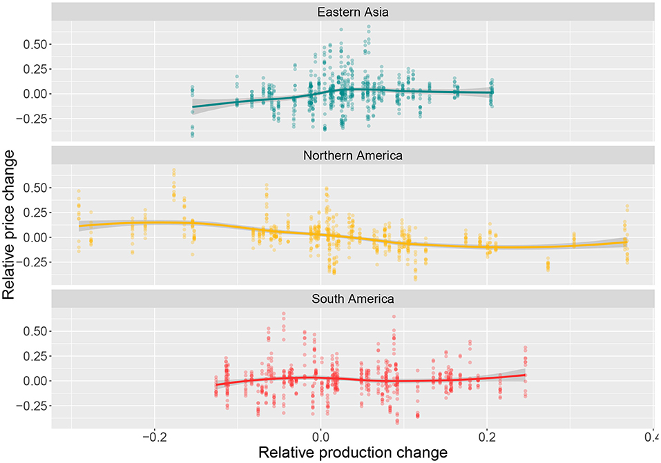
Figure 1. Annual changes (%) in global price vs. Regional production (in the three leading producing regions). Each dot represents an observation, while the smooth line (fitted using loess) shows the pattern of these two elements.

3. Methods

We consider two types of models, i.e., models predicting maize price changes as a function of yearly production (yield) changes and models predicting maize price changes from past monthly observations of price changes and yearly production (yield) changes. The first type of models can be expressed as

$\begin{array}{ll}{p}_{m,y}=f(x_{1,y},\dots ,x_{k,y},\dots ,x_{19,y})& (3)\end{array}$

and the second as:

$\begin{array}{ll}{p}_{m,y}=f(p_{m,y-1},x_{1,y},\dots ,x_{k,y},\dots ,x_{19,y})& (4)\end{array}$

where k is the region index. We consider different types of function f, based on linear models and machine learning algorithms, as described below.

3.1. Models 1, 2, and 3—Machine Learning

The use of ML makes it possible to discover hidden patterns about the relationship between the direction and magnitude of changes in p_m,y vs. the variability in x_k,y. This way, we can detect non-linear relationships between variables without making any strong preliminary assumptions on the shapes of the relationships. More specifically, we use three different approaches, namely classification and regression trees (CART, model 1), Random Forest (RF, model 2), and gradient boosting (GBM, model 3).

Classification and regression trees (CART) is a recursive ML technique developed by Breiman et al. (1984). The algorithm receives all the observations that include information about the input variables (x_1,y,x_2,y,…,x_19,y), and build a regression tree to minimize the error rate in predicting p_m,y, measured here by the residual sum of squares (RSS). The partitioning process starts with a single node at the top of the tree (root). In each step, the algorithm splits the node into two, each defined by a different input (region), and stops when no further improvement is possible, i.e., when RSS cannot be any lower. We fit CART using the rpart package of R (Therneau et al., 2019). An illustration can be found in Supplementary Figure A.b, Supplementary Data.

CART models are usually easy to interpret but are considered weak learners (Luo et al., 2019), which might be highly biased. To overcome this problem, we apply two alternative methods based on the assembly of high numbers of individual trees, namely random forest (RF) and gradient boosting machine (GBM) (Liaw et al., 2002). RF takes a random subset of the original dataset and uses it to fit a basic decision tree to predict p_m,y. A bootstrapping process is implemented T times (t = 1, …, T), and the T resulting trees are then averaged to produce the final predictions. Here, we find that RF leads to the most stable results with T = 500 trees. RF is applied here using the package randomForest (Breiman et al., 2018).

Similar to RF, GBM examines subsamples of data and fit a single tree to each one. Nevertheless, unlike the latter, the selected sub-sample is chosen according to the estimation error obtained in the analysis of the previous training set. In this study, we find that GBM returns the most accurate forecast when using T = 100 trees. This method is implemented with the gbm R package (Friedman, 2001).

3.2. Model 4—Multivariate Linear Regression

In linear model (LM), price change p_m,y is related to x_k,y as:

$\begin{array}{ll}{p}_{m,y}={\alpha }_m+{\displaystyle \sum _{k=1}^{K^s}}{\beta }_{k,m}{x}_{k,y}+{ϵ}_{m,y}& (5)\end{array}$

where α_m is the intercept, β_k,m are regression parameters, ϵ_m,y are the residuals, and K^s (< 19) is the number of selected regions. One model is fitted separately for each month m (with the function lm of the R software). To obtain a parsimonious model, we use a step-wise algorithm (based on AIC) to select the most influential K^s regions. Because of its simplicity and strong assumptions, this linear model serves as a benchmark model.

3.3. Model 5—VAR

Model vector autoregressive (VAR) empirically examines the evolution and common effects that time series have on each other so that it describes the relationships over time between all the variables in question. In this case, the model includes several dynamic variables that affect each other and the effect of shocks in each explanatory variable on the global price. Unlike the models, we have used so far, p_m,y is not only a function of x_k,y but also of the past price change values, p_m,y−1.

The basic purpose of VAR is to describe the interactions between all variables and try to predict future effects. Since firstly introduced by Sims (1980), VAR has been widely used and is considered a particularly effective tool in designing policy strategies (Bernanke et al., 2005; Jouchi et al., 2011). Here, we use this approach to predict p_m,y as a function of p_m,y−1 and of x_k,y as follows:

$\begin{array}{ll}{p}_{m,y}={\alpha }_m+{\beta }_{0,m}{p}_{m,y-1}+{\displaystyle \sum _{k=1}^K}{\beta }_{k,m}{x}_{k,y}+{ϵ}_{m,y}& (6)\end{array}$

One separate model is fitted for each month m using the vars R package (Pfaff and Stigler, 2018).

3.4. Model 6—TBATS

The Trigonometric Seasonal Box Transformation with ARMA residuals Trend and Seasonal Components (TBATS) model (De Livera et al., 2011) is an upgraded time-series model which can deal with trends, multiple-seasonality and auto-correlations. This method automatically determines whether a Box-Cox transformation of the data is required, whether seasonality needs to be accounted for (based on Fourier series), and whether a time trend should be included. It also automatically selects the optimal number of autoregressive and moving average components for predicting the target response variable.

Contrary to the models mentioned above, TBATS is fitted to the time series of the relative annual change in the monthly price of maize directly, without using the production data. TBATS aims at predicting price changes from the past series of observed price changes without taking regional productions into account. We consider several time horizons for price change predictions, from one month ahead to one year ahead. Here, this method is implemented with the R package forecast (Hyndman et al., 2020).

4. Model Evaluation

The model prediction errors were assessed and compared using a rolling cross-validation (CV) technique, implemented separately for each month and model. At each iteration of the CV, we select a sub-sample (training-set) containing observations from all the first Ỹ = 44 years (1962/3-2006/7) plus the i following years (i is successively set equal to 1, 2, …I, where I = 13 or 14, depending on the month considered). At each iteration, the training set trains the models, and the resulting trained models are used to predict the price change at year Ỹ + i + 1. With this procedure, we ensure that at least Ỹ + 1 years of data are available to train the models. Smaller datasets would lead to inaccurate predictions and a lack of identifiability.

We define the forecast error for the model in month m of the marketing year y as:

$\begin{array}{ll}{ϵ}_{m,y}={\tilde{p}}_{m,y}-p_{m,y}& (7)\end{array}$

where p_m,y is the observed price, and ${\tilde{p}}_{m,y}$ is the forecast made in month m of the marketing year y by any of the models considered in this study. We then use these errors to compute an RMSE for each month and each model, as:

$\begin{array}{ll}\begin{array}{c}RMS{E}_m=\sqrt{\frac{{\displaystyle {\sum }_{y=1}^I{({\tilde{p}}_{m,y}-p_{m,y})}^2}}{I}}\end{array}& (8)\end{array}$

The accuracy of TBATS predictions is evaluated by computing the RMSE criterion for 12 different time horizons, i.e., h = 1,2,…,12 months ahead. For a given year, a given month, and a given time horizon, TBATS is trained using all price data available before the month m − h, and the trained model is used to predict the value of p_m,y (Ỹ = 28, I_TBATS = 690). This procedure is repeated relative to every year, every month, and time horizon. Then, a specific value of RMSE has computed for each month m and time horizon h combination by averaging the prediction errors among all years of data.

Finally, we assess and rank the influences of the producing regions using two different techniques. First, we use permutation ranking with RF and GBM to assess the importance of each region for predicting maize prices. This approach allows us to identify the most and least influential regions when forecasting maize price changes (Supplementary Data). Second, using the Shapley decomposition technique (Shapley, 1953), we strive to identify the regional production variations responsible for specific extreme price change anomalies that occurred at some specific months and years in the past. Importance ranking and Shapley decomposition were implemented using the package iml of the R software.

5. Results

Figure 2 below presents a comparison between the price changes predicted by the different models and the observed price changes.

FIGURE 2

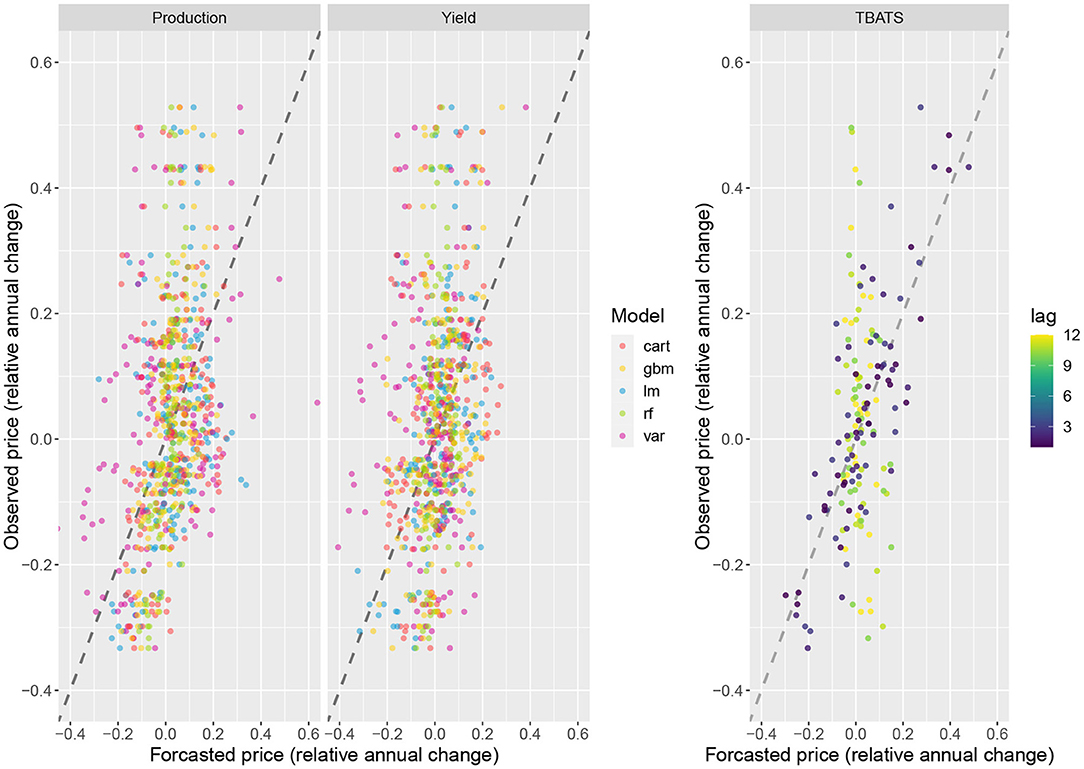
Figure 2. Maize global price change: observed vs. forecasted, as obtained with all models. CART, RF, GBM, LM, and VAR are shown on the left. The TBATS forecasts are displayed on the right for time lag ranging from 1 to 12 months. The dashed black lines are the 1:1 lines (lines of equality).

The left side of the Figure 2 presents the forecasts derived from the ML and linear models from October 2006 to January 2020 (Segmentation by months is in Supplementary Data). Generally, ML models tend to produce more accurate predictions than LM and VAR, as the latter two methods produce somewhat fluctuating predictions. Nonetheless, VAR seems to perform well in case of extreme price shocks.

TBATS predictions tend to diverge more from the observations when derived several months before the dates of forecast (right side of Figure 2). For lag longer than three months, the predictions differ a lot from the observations.

Figure 3 below shows the relative advantage of using each model for forecasting p_m,y, with the reference value being the observed standard deviation of the price each month (sd(p_m,y)). This measure corresponds to the difference between sd(p_m,y) and the RMSE of each model the same month, divided by sd(p_m,y), and expressed in percentages. A positive value indicates that the corresponding model is better than a constant prediction equal to zero. All the points below the black horizontal line indicate models offering no-better-than-average price forecasts. In contrast, those above indicate models with average forecast errors lower than sd(p_m,y). Such models are better than a constant prediction. The highest relative advantage values (located at the top of the graphic) indicate the most relevant models, which appear to be the tree-based methods in most cases (GBM, RF, and CART). The results are presented separately for TBATS to assess the influence of the time lags on the prediction accuracy. The relative advantage of TBATS compared to a constant prediction is high for a time horizon up to 3 months and became very low after six months.

FIGURE 3

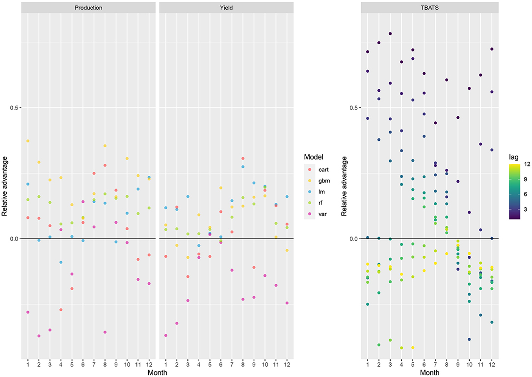
Figure 3. Relative advantage in terms of prediction accuracy of the forecasting models, over 1990–2020. This measure corresponds to the difference between the standard deviation of the price changes in the whole dataset (sd(p_m,y)) and the RMSE of each model the same month, divided by sd(p_m,y), and expressed in percentages. It indicates the relative benefit of using the models compared to a constant prediction equal to zero. ML methods, LM and VAR were used with production and yield inputs, successively.

Results show that several models are more accurate than constant predictions. The relative advantages of GBM tend to be higher when including regional productions as inputs rather than regional yields. However, the differences between the two types of inputs are not very high. The relative advantages of LM or VAR are often negative, revealing that these methods do not often perform better than constant predictions. Concerning TBATS (Figure 3, right), price change predictions are more accurate than constant predictions, as long as the time-horizon for forecasting remains lower than 3 or 4 months. For such cases (dark points in Figure 3), the relative advantage of TBATS predictions can be higher by 78% higher than constant predictions. On the other hand, for longer time horizons, the accuracy of TBATS decreases rapidly and becomes inaccurate for time lag higher than six months.

We used the cross-validated values of RMSE to identify the most accurate models for each time horizon between one month and a year ahead, as shown in Table 1.

TABLE 1

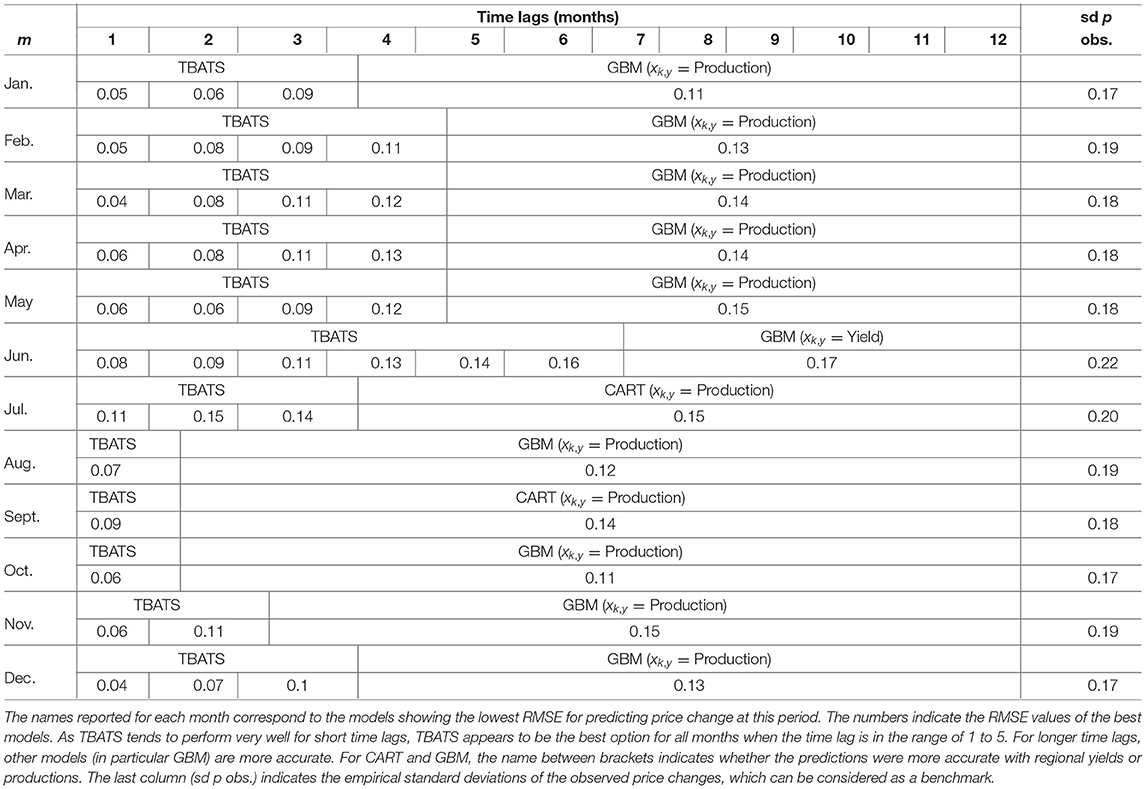
Table 1. Best forecasting options for different months.

According to Table 1, TBATS is the best model to predict p_m,y in each of the 12 months of the year in a forecast range of two (September to November) to five months ahead (February March, and May to August). However, to predict a price for time horizons longer than three or four months, ML models are often more reliable and, in addition, offer the possibility to identify the most and least influential regions based on importance ranking and Shapley decomposition. For example, importance rankings (Supplementary Figure A.b in Supplementary Data) reveal a strong influence of Northern America for almost all months. Correspondingly, Western Asia, another key producing region, had strong relative influence substantially during the two months preceding the harvest season in Northern America (July and August).

The Shapley decompositions confirm the strong influence of Northern America. Two Shapley decompositions are shown in Figure 4 for two extreme events corresponding to a substantial price increase and a strong price decrease over the period considered. Each regional Shapley value indicates the share of the price anomaly (either in December 1995 or in December 2013) explained by the corresponding region. According to these decompositions, the high maize price increase occurring in December 1995 appears to be mainly due to the changes in maize production in Northern America and, to a lower extend, in Southern Africa. The maize productions in Northern America are also responsible for a significant share of the substantial price decrease in December 2013. Other examples confirming the significant role of Northern America are shown in Supplementary Data.

FIGURE 4

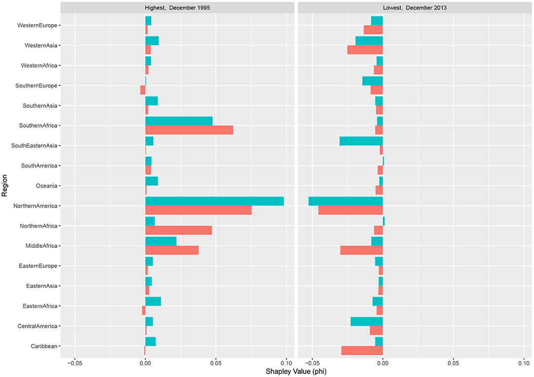
Figure 4. Shapley values for December 1995 (strong price increase) and December 2013 (strong price decrease). The decompositions show the contributions of the producing regions to two extreme relative price changes (regional production in red, and yields in blue). At a given date, the sum of the regional Shapley values is equal to the price change anomaly.

6. Discussion

This research project analyzes six decades of the global maize market. Maize is the highest produced crop worldwide and an essential energy source, especially in developing countries. Our study attempts to forecast the international monthly price of this commodity as a function of regional productions. Although many have analyzed and attempted to predict maize price accurately (Hoffman et al., 2015; Ahumada and Cornejo, 2016; Xiaojie and Yun, 2021), very few have developed methods that are both easy to reproduce and interpret by users who are not necessarily specialists in price prediction. With regards to ML, our study offers a double contribution. It is one of the first performing Medium Term maize price forecasting using ML, let alone detecting the main drivers for maize price changes through investigation of the ML algorithms. Second, it offers a practical, non-academic contribution—by providing a range of price forecasting tools that could be easily implemented by stakeholders who do not have access to the best tools needed to trade in global markets optimally.

Our study uses machine-learning algorithms and relies on publicly available data only. It is based on the use of annual regional yields and productions to enable the user to interpret the results, principally challenging the transparency of each model. The chosen models were those which had been previously tested in relation with the global maize market and regional production (Zelingher et al., 2021), i.e., CART (Breiman et al., 1984), RF (Hastie et al., 2009), and GBM (Friedman, 2001). To those are added two econometric models, each having some advantages: VAR (Sims, 1980), which can detect inter-and intra-effects of local productions shocks, and TBATS (De Livera et al., 2011), as a time-series based approach that has proved to achieve low forecasting errors (Lima and Laporta, 2020).

To understand the process behind the model outputs and identify the forces which drive price change forecasts, we use two evaluation techniques: a relative importance ranking and Shapley decomposition (Shapley, 1953). These two model-agnostic approaches are helpful to identify different drivers of maize price variations. At first, the relative importance ranking quantifies the impact of each producing region on annual changes in the monthly price (as a consequence of its contribution to the forecasting ability of the model). Next, Shapley decomposition provides a case-explicit examination of the contributions of different regional production changes to specific yearly price changes. This second approach is especially relevant for understanding the forces influencing extreme price changes, which might drive a global food crisis.

The paper emphasizes the importance quantifying the marginal contribution of each input factor used to forecast price changes. Furthermore, this study highlights the importance of predicting global maize prices according to various scenarios using different models. This way, the impact of the various producing regions (input) can be examined and evaluated accordingly. This approach provides valuable information for understanding the impacts of production changes in highly influential regions.

Our results reveal significant dissimilarities between the impact levels of the different regions. Our results confirm the existence of strong relationships between maize prices and production changes in major producing regions, as already claimed by Headey and Fan (2010). However, the strength of these relationships varies over time and is stronger in the months and weaker in others. Thus, the impact of Northern America is strong throughout the entire year except for July and August. As it happens, the primary harvest season in this region begins in September and, after this month, the previous year's crop is no longer traded or only in small volumes. As it is not yet possible to predict with certainty the amount of crop harvested in the coming year, the impact of Northern America declines in July-August. On the opposite, the relative impact of Western Asia becomes higher in July and August, as these two months present the main harvest season in this region.

This study offers a significant contribution to the price forecasting literature of agricultural commodities. First and foremost, our modeling framework is constructed to be easily replicated. Whereas, to date, many have been obliged to base their food security strategy on paid data obtained from private companies or based on results that are difficult to replicate (see WASDE, World Bank Commodities Price Forecast or FAO-AMIS Market Database); our research offers an interesting alternative. Indeed, our codes provide the users with tools to predict maize price values and to understand the processes leading to these forecasted price values. Another contribution derives from the division of the forecasting period simultaneously to months and time horizon, giving the users the unique opportunity to adapt their strategy in case of possible changes in the maize market. Lastly, our approach enables analysis of specific events through the Shapley-algorithm, while taking the opportunity to understand the origins of extreme price changes.

Although this project deals with maize, the tested methodologies can be applied to other agricultural commodities. In future work, we will examine this assumption on several different internationally traded crops. There, we will strive to capture inter-and intra-sectoral differences, detect the factors impacting price volatilities, expand our forecasting tools to a larger set of commodities, and contribute to increase global food security.

Data Availability Statement

The original contributions presented in the study are included in the article/Supplementary Material, further inquiries can be directed to the corresponding author/s.

Author Contributions

All authors listed have made a substantial, direct, and intellectual contribution to the work and approved it for publication.

Funding

This study was funded by the French ANR project CLAND (16-CONV-0003) and by the INRAE metaprogram GloFoods.

Conflict of Interest

The authors declare that the research was conducted in the absence of any commercial or financial relationships that could be construed as a potential conflict of interest.

Publisher's Note

All claims expressed in this article are solely those of the authors and do not necessarily represent those of their affiliated organizations, or those of the publisher, the editors and the reviewers. Any product that may be evaluated in this article, or claim that may be made by its manufacturer, is not guaranteed or endorsed by the publisher.

Supplementary Material

The Supplementary Material for this article can be found online at: https://www.frontiersin.org/articles/10.3389/fsufs.2022.836437/full#supplementary-material

References

Ahumada, H., and Cornejo, M. (2016). Forecasting food prices: the case of corn, soybeans and wheat. In. J. Forecast. 32, 838–848. doi: 10.1016/j.ijforecast.2016.01.002

CrossRef Full Text | Google Scholar

Barrett, C. B. (2002). “Food security and food assistance programs,” in Agricultural and Food Policy, Handbook of Agricultural Economics, Vol. 2 (Ithaca, NY: Elsevier), 2103–2190.

PubMed Abstract | Google Scholar

Bellemare, M. F., Barrett, C. B., and Just, D. R. (2013). The welfare impacts of commodity price volatility: evidence from rural ethiopia. Am. J. Agric. Econ. 95, 877–899. doi: 10.1093/ajae/aat018

CrossRef Full Text | Google Scholar

Bernanke, B. S., Boivin, J., and Eliasz, P. (2005). Measuring the effects of monetary policy: a factor-augmented vector autoregressive (favar) approach*. Quart. J. Econ. 120, 387–422. doi: 10.3386/w10220

CrossRef Full Text | Google Scholar

Breiman, L., Cutler, A., Liaw, A., and Matthew, W. (2018). Breiman and Cutler's Random Forests for Classification and Regression, R Package Version 4.6-14. Berkeley, CA: UC Berkeley.

Breiman, L., Friedman, J., Stone, C. J., and Olshen, R. A. (1984). Classification and Regression Trees. Monterey, CA: CRC Press.

Google Scholar

De Livera, A. M., Hyndman, R. J., and Snyder, R. D. (2011). Forecasting time series with complex seasonal patterns using exponential smoothing. J. Am. Stat. Assoc. 106, 1513–1527. doi: 10.1198/jasa.2011.tm09771

PubMed Abstract | CrossRef Full Text | Google Scholar

ERS-USDA (2021). Food Price Outlook. Washington, DC: USDA.

Google Scholar

FAO (2020). FAOSTAT Statistical Database. FAO, Rome.

Friedman, J. H. (2001). Greedy function approximation: a gradient boosting machine. Ann. Stat. 29, 1189–1232. doi: 10.1214/aos/1013203451

CrossRef Full Text | Google Scholar

Hastie, T., Tibshirani, R., and Friedman, J. (2009). Random Forests. New York, NY: Springer, 587–604.

Google Scholar

Headey, D., and Fan, S. (2010). Reflections on the Global Food Crisis: How Did It Happen? How Has It Hurt? and How Can We Prevent the Next One?. Washington, DC: International Food Policy Research Institute. doi: 10.2499/9780896291782RM165

CrossRef Full Text | Google Scholar

Henneberry, D., and Kargbo, J. (1986). Structural Overview of the World Corn Market. Technical Report, Oklahoma Cooperative Extension Service, Oklahoma City, OK.

Google Scholar

Hertel, T. W., Baldos, U. L. C., and van der Mensbrugghe, D. (2016). Predicting long-term food demand, cropland use, and prices. Ann. Rev. Resour. Econ. 8, 417–441. doi: 10.1146/annurev-resource-100815-095333

CrossRef Full Text | Google Scholar

Hoffman, L., and Meyer, L. (2018). Forecasting the US Season-Average Farm Price of Upland Cotton: Derivation of a Futures Price Forecasting Model. Technical Report CWS-18I-01, USDA ERS, Washington, DC.

Google Scholar

Hoffman, L. A. (2011). Using Futures Prices to Forecast US Corn Prices: Model Performance With Increased Price Volatility, Ch. 7. New York, NY: Springer, 107–132.

Google Scholar

Hoffman, L. A., Etienne, X. L., Irwin, S. H., Colino, E. V., and Toasa, J. I. (2015). Forecast performance of wasde price projections for us corn. Agric. Econ. 46, 157–171. doi: 10.1111/agec.12204

CrossRef Full Text | Google Scholar

Hyndman, R., Athanasopoulos, G., Caceres, G., Chhay, L., O'Hara-Wild, M., Petropoulos, F., et al. (2020). Forecasting Functions for Time Series and Linear Models. NA. R Package Version 8.12.

Jouchi, N., Munehisa, K., and Toshiaki, W. (2011). Bayesian analysis of time-varying parameter vector autoregressive model for the japanese economy and monetary policy. J. Jpn Int. Econ. 25, 225–245. doi: 10.1016/j.jjie.2011.07.004

CrossRef Full Text | Google Scholar

Liaw, A., and Wiener, M. (2002). Classification and regression by randomforest. R News 2, 18–22.

Google Scholar

Lima, M. V. M. D., and Laporta, G. Z. (2020). Evaluation of the models for forecasting dengue in brazil from 2000 to 2017: an ecological time-series study. Insects 11, 1–14. doi: 10.3390/insects11110794

PubMed Abstract | CrossRef Full Text | Google Scholar

Luo, Z., Bui, X.-N., Nguyen, H., and Moayedi, H. (2019). A novel artificial intelligence technique for analyzing slope stability using pso-ca model. Eng. Comput. 37, 1–12. doi: 10.1007/s00366-019-00839-5

PubMed Abstract | CrossRef Full Text | Google Scholar

Lusk, J. L. (2016). From Farm Income To Food Consumption: Valuing Usda Data Products. Technical Report 643-2018-161, Council on Food, Agricultural and Resource Economics (C-FARE).

Google Scholar

Natanelov, V., McKenzie, A. M., and Van Huylenbroeck, G. (2013). Crude oil–corn–ethanol – nexus: a contextual approach. Energy Policy, 63:504–513. doi: 10.1016/j.enpol.2013.08.026

CrossRef Full Text | Google Scholar

Pfaff, B., and Stigler, M. (2018). Package ‘vars.' Kronberg im Taunus. R Package Version 1.5-3.

Google Scholar

Piot-Lepetit, I., and M'Barek, R. (2011). Methods to Analyse Agricultural Commodity Price Volatility. New York, NY: Springer. 1–11.

Google Scholar

Schaub, S., and Finger, R. (2020). Effects of drought on hay and feed grain prices. Environ. Res. Lett. 15, 034014. doi: 10.1088/1748-9326/ab68ab

CrossRef Full Text | Google Scholar

Shapley, L. (1953). “A value for n-person games,” in Contributions to the Theory of Games II, eds H. Kuhn and A. Tucker (Princeton, NJ: Princeton University Press), 307–317. doi: 10.1515/9781400881970-018

CrossRef Full Text | Google Scholar

Sims, C. A. (1980). Macroeconomics and reality. Econometrica 48, 1–48.

Google Scholar

Therneau, T., Atkinson, B., Ripley, B., and Ripley, M. B. (2019). Package ‘rpart.' CRAN. R Package Version 4.1-15.

Google Scholar

Valin, H., Sands, R. D., van der Mensbrugghe, D., Nelson, G. C., Ahammad, H., Blanc, E., et al. (2014). The future of food demand: understanding differences in global economic models. Agric. Econ. 45, 51–67. doi: 10.1111/agec.12089

CrossRef Full Text | Google Scholar

Warr, P. G. (1990). Predictive performance of the world bank's commodity price projections. Agric. Econ. 4, 365–379.

Google Scholar

Xiaojie, X., and Yun, Z. (2021). Corn cash price forecasting with neural networks. Comput. Electron. Agric. 184, 106120. doi: 10.1016/j.compag.2021.106120

CrossRef Full Text | Google Scholar

Zelingher, R., Makowski, D., and Brunelle, T. (2021). Assessing the sensitivity of global maize price to regional productions using statistical and machine learning methods. Front. Sustain. Food Syst. 5, 171. doi: 10.3389/fsufs.2021.655206

CrossRef Full Text | Google Scholar