A fast hyperspectral change detection algorithm for agricultural crops based on low-rank matrix and morphological feature extraction

1 Introduction

Achieving sustainable agricultural productivity and global food security are two of the biggest challenges of the new millennium (Wang et al., 2022). Studying crop change detection is the foundation of agricultural sustainability, contributing to enhancing the resilience of agricultural systems reducing production risks, improving the livelihoods of rural communities, thus ensuring the sustainability of food supply. Change detection, a pivotal application in remote sensing, is essential for continuously monitoring and identifying alterations in remote sensing image scenes (Hasanlou and Seydi, 2018; Liu et al., 2019; Hou et al., 2021), which has been widely applied in environmental monitoring, land change analysis, urban expansion assessment, disaster detection and evaluation, and military battlefield monitoring, and provides valuable insights (Eismann et al., 2007; Wu et al., 2013; Xia et al., 2024). Crop change detection, in particular, holds significant importance. The timely and accurate acquisition of crop sowing change information is crucial for developing national/regional agricultural economic plans, guiding structural adjustments in the planting industry, and enhancing agricultural production management.

Unlike high-resolution remote sensing images (Ma et al., 2023, 2024), hyperspectral images (HSIs) organize data into three-dimensional (3D) cubes with both spatial and spectral dimensions, providing intricate spectral “diagnostic” information (Ren et al., 2023). This unique capability, coupled with its inherent advantages such as wide coverage and short detection periods (Liu et al., 2014; Marinelli et al., 2019), holds immense potential for accurate crop change detection and the identification of various types of agricultural transformations (Song et al., 2018).

Various methodologies have been proposed, thoroughly reviewed, categorized, and analyzed for hyperspectral image (HSI) change detection across diverse applications (Liu et al., 2019; Vali et al., 2020). HSI change detection is commonly classified into four main groups:

1. Algebra-based methods: This category encompasses techniques such as image differencing, ratioing, regression, absolute distance (AD; Du et al., 2012), and change vector analysis (CVA; Ghamisi et al., 2017). These methods are simple and efficient, yet their fundamental assumption is that changes result in noticeable differences in pixel gray level values.

2. Transformation-based methods: Techniques like conventional principal component analysis (CPCA), temporal principal component analysis (TPCA; Nielsen et al., 1998), multivariate alteration detection (MAD), and independent component analysis fall into this group. They project hyperspectral data into alternative feature spaces to identify changed pixels, but may overlook continuous spectral signatures and pixel similarity.

3. Classification-based methods: This category involves post-classification or direct classification methods applied to multitemporal images (Bovolo et al., 2008; Demir et al., 2012). Post-classification entails separate classification of images from different time series, eliminating the impact of environmental factors. Direct classification treats multitemporal images collectively, using a classifier to identify changed categories (Khanday and Kumar, 2016; Wang et al., 2018; Hu et al., 2023). However, they demand a higher level of sophistication in classification algorithms.

4. Other advanced methods: This group comprises unmixing-based (Zhang et al., 2011; Ertürk et al., 2016; Liu et al., 2016), low-rank and sparse representation-based (Wu et al., 2018), and deep learning-based approaches (Hong et al., 2021; Huang et al., 2022; Song et al., 2022; Luo et al., 2023; Wang et al., 2023); Deep learning methods aim to generate data-driven transformations for advanced feature extraction, with their effectiveness dependent on the scale and accuracy of training databases (Lin et al., 2019; Gao et al., 2020; Zheng et al., 2020; Li et al., 2022; Yang et al., 2023).

Although various algorithms mentioned above have demonstrated excellent performance in different fields (Zhou et al., 2016; Seydi et al., 2021; Seydi and Hasanlou, 2021), they still face challenges in practical applications due to factors such as seasons, terrain, and weather conditions, including: (1) Interference from abnormal pixels; (2) Limited versatility in detection methods; and (3) Underutilization of spatial information during detection. Consequently, the focal point in hyperspectral change detection research is to enhance the differentiation between changed pixels and the background while accurately distinguishing changed pixels from the background (Ortiz-Rivera et al., 2006; Zhan et al., 2020).

In recent years, sparse representation has proven to be a powerful tool for interpreting hyperspectral images (Li et al., 2016; Ghasemian and Shah-Hosseini, 2020; Peng et al., 2021). Among these, low-rank and sparse matrix decomposition methods leverage the intrinsic properties of HSIs (Bouwmans et al., 2016; Wu et al., 2019; Xie et al., 2019). They decompose pixels with sparse characteristics representing changes from those with low-rank characteristics representing unchanged elements, and effectively eliminating noise. Such methods enable modeling of spectral signals without assuming or estimating specific statistical distributions, which can be particularly useful for modeling change trends. Simultaneously, morphological feature extraction has been proven to be a powerful tool in fields such as crop classification and detection (Bosilj et al., 2018; Li et al., 2023). Expressing the topological structure and morphological attributes among crops enables the introduction of spatial information, forming a more universally applicable and effective method for detecting agricultural changes.

The spectral-spatial information is of great importance for change detection (Mou et al., 2018). Change detection based on it aims at extracting not only the spatial information but also explore the underlying information of the spectral features to obtain a better performance (Zhang and Lu, 2019). Based on the above discussions, this paper introduces a fast hyperspectral change detection approach for agricultural crops based on low-rank matrix and morphological feature extraction (FLRaMF). The proposed method takes a two-fold approach. Firstly, it preliminarily separates changed and unchanged pixels in the spectral domain by extracting a low-rank matrix. Secondly, it effectively captures and utilizes the spatial characteristics of crops through Attribute Profiles (AP). The integration of spectral-spatial information yields reliable change detection results for dual-temporal agricultural crops. In this study, the FLRaMF method exhibits outstanding performance when applied to four real dual-temporal hyperspectral change detection datasets for agricultural crops. The primary contributions of this research are succinctly summarized as follows.

1. FLRaMF is a non-supervised change detection method, which eliminates the need of prior knowledge and samples in agricultural change detection. Simultaneously, after carefully considering the data characteristics of such scenes, the algorithm’s parameters are simple, and the default settings exhibit broad applicability.

2. The proposed method fully exploits the topological features and spatial morphology of agricultural crops, addressing the issue of poor detection performance caused by interference from abnormal pixels in the spectral domain. This enhancement further improves the performance of change detection.

3. The proposed method introduces a greedy bilateral smoothing model which better separates changed pixels from unchanged pixels considering the intrinsic characteristics of the data, significantly enhancing the operational efficiency of the algorithm.

The paper is structured as follows: Section 2 introduces the datasets, the basic concepts of AP and LRaSMD and the proposed algorithm. Section 3 presents the experiments conducted with four datasets and analysis. Finally, section 4 summarizes the entire study.

2 Materials and methods

Four real dual-temporal hyperspectral datasets related to agricultural crops was used to validate the effectiveness of the proposed FLRaMF algorithm.

2.1 Materials

2.1.1 The Bay Area dataset

The Bay Area dataset was collected in Patterson, California, United States. These images were acquired using the AVIRIS sensor in 2013 and 2015, with high-spectral remote sensing image dimensions of 500 × 600 for both periods, comprising a total of 224 bands. The Bay Area dataset primarily includes farmland and urban areas. Due to the complexity of urban changes, the ground truth map in terms of changed and unchanged regions mainly focuses on farmland areas. In the ground truth map, white pixels represent unchanged elements, gray pixels represent changed elements, and black pixels represent elements where changes were not determined.

2.1.2 The Santa Barbara dataset

The Santa Barbara dataset is located in the Santa Barbara region of California, United States. These images were captured using the AVIRIS sensor in 2013 and 2014, with high-spectral remote sensing image dimensions of 740 × 984 for both periods, comprising a total of 224 bands. The Santa Barbara dataset primarily includes mountainous and farmland areas. In the ground truth map, white pixels represent unchanged elements, gray pixels represent changed elements, and black pixels represent elements where changes were not determined. Analysis of the ground truth map for the Santa Barbara dataset reveals that the upper part of the mountainous area is labeled as unchanged elements, and since this area contains a variety of land cover types, high demands are placed on the interference resistance of hyperspectral remote sensing change detection algorithms.

2.1.3 The Hermiston dataset

The Hermiston dataset is located in Hermiston, Oregon, United States, covering farm and river regions. Images were acquired using the Hyperion sensor in 2004 and 2007, with high-spectral remote sensing image dimensions of 200 × 390 for both periods, comprising a total of 242 bands.

2.1.4 The Farmland dataset

The Farmland dataset was collected using the Hyperion sensor, capturing farmland in Yancheng City, Jiangsu Province, China. These images were obtained in May 2006 and April 2007, with dimensions of 140 × 420, and a total of 154 bands after removing the noisy bands.

The pseudo color prevent, postevent HSIs and the groundtruth changes of different datasets are depicted, respectively (Figures 1–4), specific parameters of which is given (Table 1). The experimental platform is a computer equipped with an Intel (R) Core(TM) i7-8750H CPU (2.20 GHz) and 16GB RAM, and all programs are implemented in MATLAB R2018a.

Figure 1

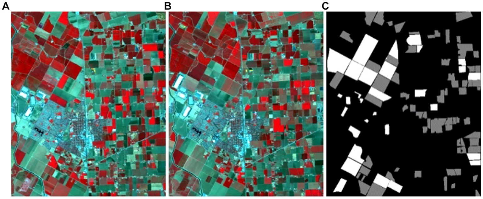
Figure 1. Illustration of the Bay Area dataset. (A) Bay Area scene on 2013, (B) Bay Area scene on 2014, (C) Ground-truth change map.

Figure 2

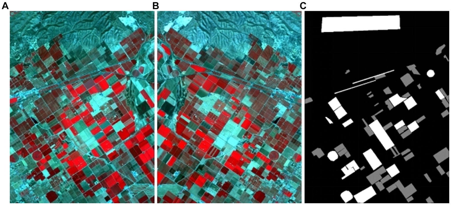
Figure 2. Illustration of the Santa Barbara dataset. (A) Santa Barbara scene on 2013, (B) Bay Area scene on 2015, (C) Ground-truth change map.

Figure 3

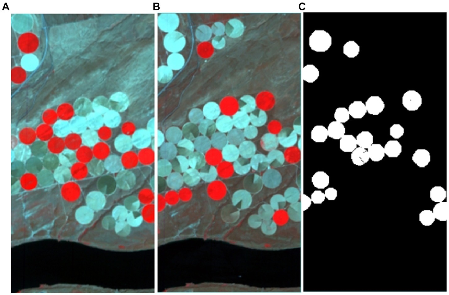
Figure 3. Illustration of the Hermiston dataset. (A) Farmland on 1 May 2004, (B) Farmland on 8 May 2007, (C) Ground-truth change map.

Figure 4

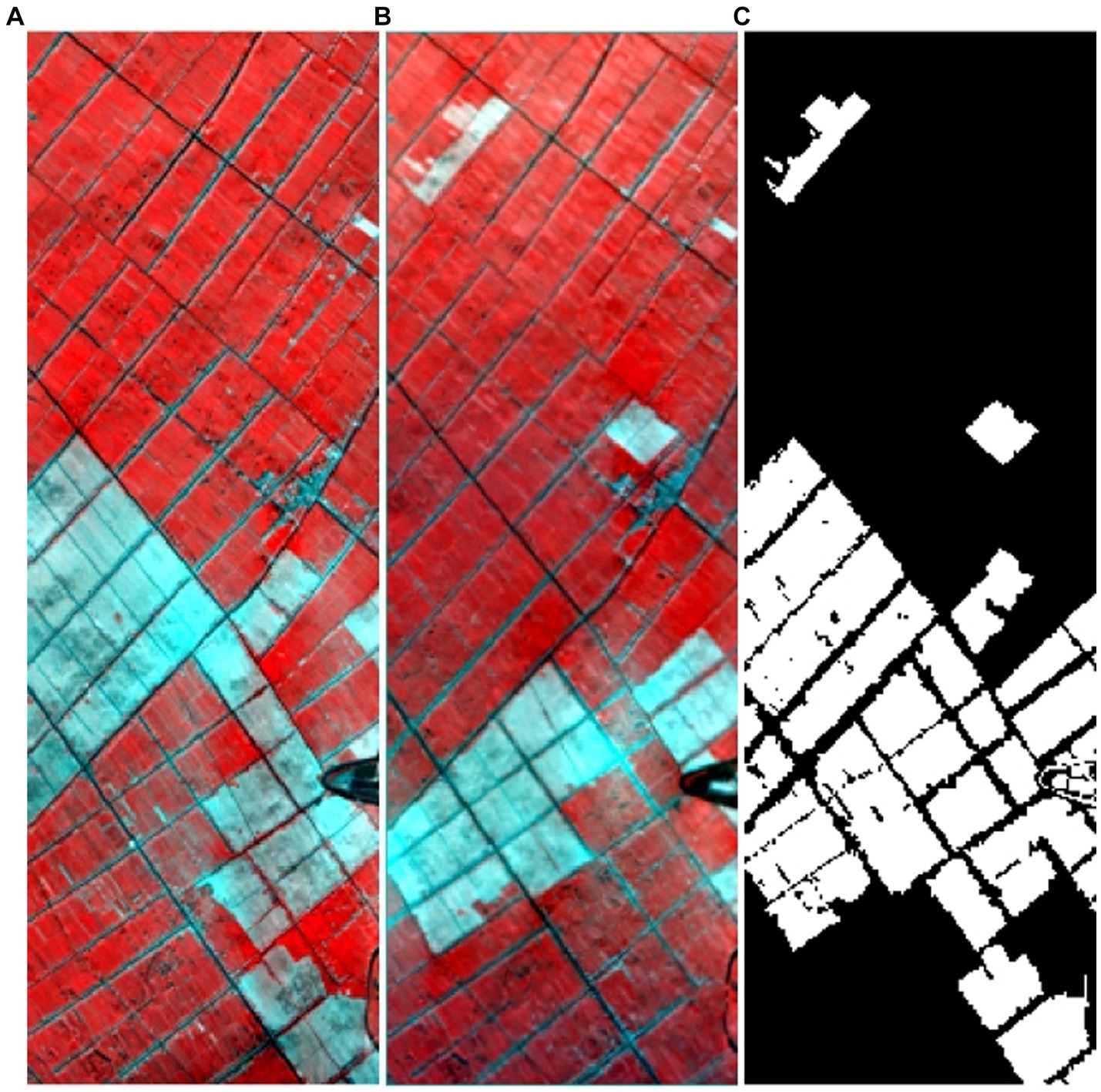
Figure 4. Illustration of the Yancheng dataset. (A) Farmland on 3 May 2006, (B) Farmland on 23 April 2007, (C) Ground-truth change map.

Table 1

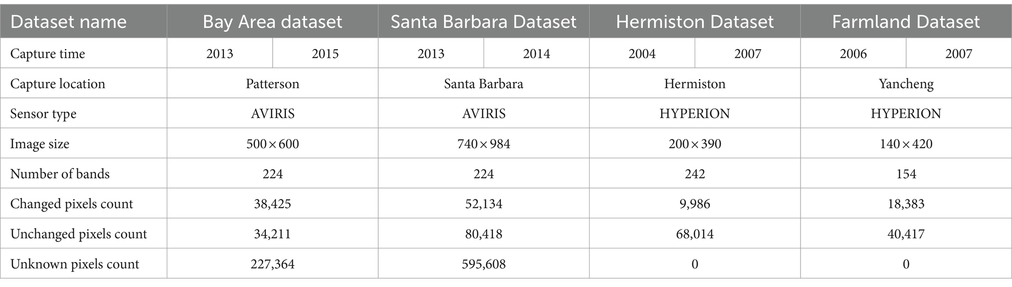
Table 1. Detailed parameters of the dataset.

2.2 Methods

2.2.1 Low-rank and sparse matrix decomposition

In hyperspectral data, the spectral vectors of neighboring pixels exhibit similarity due to shared characteristics (Zhang et al., 2013). Owing to the strong inter-band correlations, the spectral vectors of smooth and continuous background pixels in hyperspectral images (HSI) can be effectively approximated as linear combinations of a few base vectors. Consequently, the HSI background is characterized by low rankness within a low-dimensional subspace. Conversely, anomalous pixels constitute a minor fraction of the image and, assuming a random distribution, exhibit sparsity. The LRaSMD (Low-Rank and Sparse Matrix Decomposition) method represents the matrix as the sum of low-rank, sparse, and noise matrices. This approach effectively captures the low-rankness and sparsity associated with HSI background and anomalous features. Unlike aiming to establish individual models for each feature, the LRaSMD method concurrently considers both feature types. It extracts valuable information from noise and retrieves additional background components from restored data. The LRaSMD algorithm is mathematically formulated by Equation (1) (Zhou and Tao, 2011).

$\begin{array}{ll}X=B+A+N& (1)\end{array}$

where $X\in {\mathbb{R}}^{n\times b}$ represents the spectral value of the nth pixel in the bth band. B is the low-rank matrix representing the spectral information for the image background. A is the sparse matrix representing the spectral information for the changing target. N is the noise matrix, and the noise in the image is assumed to follow a Gaussian distribution.

The algorithm minimizes the decomposition error function by controlling model complexity, restricting the rank of the low-rank matrix B, and ensuring the sparsity of the sparse matrix A. This process results in the rewriting of Equation (1) as Equation (2).

$\begin{array}{c}\hfill min{‖X-B-A‖}_F^2,\mathit{rank}\left(B\right)\le r\hfill \\ \hfill \mathit{card}\left(A\right)\le kn\hfill \end{array}\text{ (2)}$

In Equation (2), r and k represent the rank of the low-rank matrix and the sparsity of the sparse matrix, respectively. This equation effectively conveys background information by controlling the maximum value of r, while k expresses the occurrence probability of anomalous pixels in the image. With an increasing number of iterations, the decomposition error consistently decreases. Consequently, Equation (2) can be decomposed into two sub-problems, and their functions are detailed in Equation (3).

$\begin{array}{l}{B}_t=\underset{\mathit{rank}\left(B\right)\le r}{\mathrm{argmin}}{\Vert X-B-A_{t-1}\Vert }_F^2\hfill \\ S_t=\underset{\mathit{card}\left(A\right)\le kn}{\mathrm{argmin}}{\Vert X-B_{t-1}-A\Vert }_F^2\hfill \end{array}\text{ (3)}$

Upon uniform convergence of decomposition errors to a local minimum, the iteration halts, and the low-rank matrix B, sparse matrix A, and noise matrix N are constructed.

2.2.2 Attribute profiles

Attribute profiles (APs) originate from the morphological profile (Pesaresi and Benediktsson, 2001). APs are based on attribute filters that operate using an image’s connected components (CC). Through two basic operators, thinning and thickening, filtration produces a series of image sequences. This process compares each CC’s attributes and threshold value, and then estimates whether this region satisfies the set standard. If not, the value is set to the nearest radiation value in the adjacent domain, merging that region into the adjacent CC. This domain can be merged into an adjacent domain with a lower or higher grayness level, resulting in thinning and thickening, respectively. The function underlying this process is given by Equation (4).

Attribute profiles (APs) are derived from the morphological profile (Dalla Mura et al., 2010) and rely on attribute filters that operate based on connected components (CC) within an image. Utilizing two fundamental operators, thinning and thickening, filtration generates a sequence of image profiles. This procedure involves assessing the attributes and threshold value$\beta$of each CC, determining whether the region meets the predefined standard. If not, the value is adjusted to the nearest radiation value in the neighboring domain, incorporating that region into the adjacent CC. This merging can occur with a lower or higher grayness level in the adjacent domain, leading to thinning and thickening, respectively. The function governing this process is expressed by Equation (4).

$\begin{array}{ll}AP\left(f\right)=\left\{{\varphi }_n\left(f\right),{\varphi }_{n-1}\left(f\right),\dots ,{\varphi }_1\left(f\right),{\gamma }_1\left(f\right),{\gamma }_2\left(f\right),\dots ,{\gamma }_n\left(f\right)\right\}& (4)\end{array}$

Where ${\gamma }_i$ and ${\varphi }_i\left(i=1,2,\dots n\right)$ represent thinning and thickening, respectively.

2.2.3 Proposed algorithm

The workflow of the FLRaMF method is illustrated (Figure 5), comprising three steps: firstly, the rapid extraction of low-rank information based on “greedy bilateral smoothing”; secondly, spatial information extraction based on Attribute Profiles (AP); and finally, the integration of spectral-spatial domain change features to obtain the ultimate detection results.

Figure 5

Figure 5. Flowchart of the method.

According to the LRaSMD method described in section 2.2.1, the model reconstructs HSI data into $X=B+A+N\left(X\in {\mathbb{R}}^{n\times b}\right)\text{.}$ To address the time cost of single-value decomposition at each iteration in the traditional LRaSMD model, a greedy bilateral smoothing method proposed by Zhou and Tao (2011) is applied to the additive noise matrix N. Here, we substitute the low-rank matrix B with the bilateral factor B = MN and apply regularization to the$\mathcal{𝓁}$1 norm of sparse matrix A. This process is expressed by Equation (5).

$\begin{array}{c}\underset{M,N,A}{min}{\Vert X-MN-A\Vert }_F^2+\lambda \Vert A\Vert {}_1\\ \mathrm{s}.\mathrm{t}.\mathit{rank}\left(M\right)=\mathit{rank}\left(N\right)\le r\end{array}\text{ (5)}$

Where $\lambda$ is a regularization parameter. To solve Equation (5), this method introduces a soft threshold $S_{\lambda }X=sgn\left(X\right)\cdot max\left(\left|X\right|-\lambda ,0\right)$ during regularization of $\mathcal{𝓁}$1 and updating of A. $S_{\lambda }$ is the soft threshold operator for $\lambda$. Alternate optimization of M, N, and A in Equation (5) leads to Equation (6).

$\begin{array}{c}{M}_k=\left(X-A_{k-1}\right)N_{k-1}^T{\left(N_{k-1}{N}_{k-1}^T\right)}^{†}\\ N_k={\left(M_k^T{M}_k\right)}^{†}{M}_k^T\left(X-A_{k-1}\right)\\ A_k=S_{\lambda }\left(X-M_k{N}_k\right)\end{array}\text{ (6)}$

Where k denotes the number of iterations. $\left(\cdot \right)†$ is the Moore-Penrose pseudo-inverse operation. Because MN and $A$ codetermine the value of Equation (5) rather than $M$ or $N$ individually, a pair of $\left(M,N\right)$ can be found with the same product as $\left(M_k,N_k\right)$ in Equation (6), leading to faster computation. Thus, Equation (6) can be rewritten as Equation (7).

$\begin{array}{ll}{M}_k{N}_k=M_k{\left(M_k^T{N}_k\right)}^{†}{M}_k^T\left(X-A_{k-1}\right)=\mathcal{P}\left(X-A_{k-1}\right)& (7)\end{array}$

Where $\mathcal{P}$ is an orthogonal projection operator. According to Equation (6), the column space of $M_k$ can be represented on a random orthonormal basis using $\left(X-A_{k-1}\right)N_{k-1}^T$ columns. Based on $\left(X-A_{k-1}\right)N_{k-1}^T=QR$, the fast $QR$ decomposition method,$M_k$is transformed into $Q$,and $M_k{N}_k$ can be computed as $M_k{N}_k={\mathcal{P}}_Q\left(X-A_{k-1}\right)=Q{Q}^T\left(X-A_{k-1}\right)$. Then, a fast upgrading process was applied, as described in Equation (8).

$\begin{array}{c}\hfill M_k=Q\hfill \\ \hfill N_k=Q^T\left(X-A_{k-1}\right)\hfill \\ \hfill A_k=S_{\lambda }\left(X-M_k{N}_k\right)\hfill \end{array}\text{ (8)}$

In the GreBsmo method, Equation (8) iterates k times or until the object converges. Then, it adds $\mathrm{\Delta }r$ rows to matrix $N$, reducing the object’s value. To determine the fastest decreasing trend, it greedily uses the added $\mathrm{\Delta }r$ rows as the singular vector of the top $\mathrm{\Delta }r$ of the partial derivative. Then, the rank of matrix $N$ is added to $r_1=r_0+\mathrm{\Delta }r$. This function is shown as Equation (9).

$\begin{array}{ll}\frac{\partial {‖X-MN-A‖}_F^2}{\partial N}=X-MN-A& (9)\end{array}$

Once reaching the set fault tolerance, the rank $r$ stops increasing.

Division into background and anomaly components can weaken the interference effect of anomalies on background statistics, so the decomposed low-rank component should be treated as an initial spectral anomaly feature.

Whether based on spectral or spatial features, change detection tends to identify similar change targets. However, due to different attribute information, different false alarms may occur. Spectral-based change detection methods may result in larger initial detection values for some background pixels, similar to anomalies, because they represent a small number of pixels. However, these pixels are often dissimilar in other attributes, such as area. To address this issue, the algorithm identifies similar changing targets and implements a strategy involving mutual inhibition of the two backgrounds. This approach effectively reduces the false alarm rate.

The initial spatial anomaly feature detection is conducted based on Mahalanobis distance, as shown in Equation (10).

$\begin{array}{ll}{X}_{\mathit{spa}}\left(x_i\right)={\left(x_i-\mu \right)}^{{\rm T}}{\Gamma }^{-1}\left(x_i-\mu \right)& (10)\end{array}$

Where $x_i={\left[x_1,x_2,\dots ,x_b\right]}^{{\rm T}}$ denotes the spatial feature vector of each pixel, $\mu ={\left({\mu }_1,{\mu }_2,\dots {\mu }_b\right)}^{{\rm T}}$ and $\Gamma$ showed, respectively, in Equations (11, 12), are the mean value and covariance matrix, respectively, of the input background data.

$\begin{array}{ll}{\mu }_b=\frac{1}{n}{\displaystyle \sum }_{i=1}^n{x}_i& (11)\end{array}$

$\begin{array}{ll}{\Gamma }_b=\frac{1}{n}{\displaystyle \sum }_{i=1}^n\left(x_i-{\mu }_b\right){\left(x_i-{\mu }_b\right)}^{{\rm T}}& (12)\end{array}$

The model implementation process can be concluded in Algorithm 1.

ALGORITHM 1: FLRaMF framework for hyperspectral change detection

Input: Hyperspectral image; rank r; rank step Δr; power K; soft thresholding $\lambda$; tolerance $\tau$;

Output: A two-dimensional detection result.

1: Initialize $N\in {\mathbb{R}}^{r_0\times n}$ and A

2: while residual error ≤$\tau$do

3: for $k=1$ to $K$ do

4: sequentially compute Eq. (8)

5: end for

6: Calculate the top Δr right singular vectors v of $\partial f/\partial M$ in Eq. (9)

7: Set $V:=\left[V;\upsilon \right]$

8: end

9: Extract the first three principal components of the original HSI

10: Calculate and obtain a set of EMAP features and extract the first four principal components;

11: Calculate preliminary detection values via Eq. (10)

2.2.4 Detection performance

In hyperspectral remote sensing image change detection, after extracting change information from the difference map, a change result map is typically utilized to represent the differential information. The change result map encompasses the change status of each pixel position. For a pixel $x_s$ defined by Equation (13) in the change result map, if it corresponds to a changed pixel $X_c$,it indicates a change; if it corresponds to an unchanged pixel $X_u$, it signifies no change:

$x_s=\{\begin{array}{l}1,x_s\in X_c\hfill \\ 0,x_s\in X_u\hfill \end{array}\text{ (13)}$

After obtaining the change result map, a crucial step involves performing a quantitative analysis of its accuracy. Commonly used metrics for this analysis include Overall Errors (OE), Percentage Correct Classification (PCC), and Kappa Coefficient. These metrics are calculated based on the counts of true positive samples (TP), true negative samples (TN), false positive samples (FP), and false negative samples (FN). The formula for calculating Overall Errors (OE) calculated through Equation (14) is as follows:

$\begin{array}{ll}OE=FN+FP& (14)\end{array}$

Overall Errors (OE) represent the total number of pixels that were not successfully detected. A smaller OE indicates fewer erroneously detected pixels, reflecting better algorithm performance.

The formula for calculating Percentage Correct Classification (PCC) is showed as Equation (15):

$\begin{array}{ll}PCC=\frac{TP+TN}{TP+TN+FP+FN}& (15)\end{array}$

The accuracy value falls within the range of [0,1], where a higher accuracy indicates a greater number of correctly detected pixels, reflecting higher algorithm precision.

The Kappa Coefficient can be calculated based on PCC, and its formula is given by Equation (16):

$\begin{array}{ll}\mathit{Kappa}=\frac{PCC-PRE}{1-PRE}& (16)\end{array}$

The calculation formula as Equation (17) shows for PRE is:

$\begin{array}{ll}PRE=\frac{N_c\times \left(TP+FP\right)+N_u\times \left(TN+FN\right)}{\left(TP+FP+TN+FN\right)}& (17)\end{array}$

The formula above is where $N_c$ represents the total number of actual changed pixels, and$N_u$represents the total number of actual unchanged pixels. The Kappa coefficient ranges from [0,1], and a higher Kappa value indicates higher accuracy in change detection.

3 Results and discussion

3.1 Experimental results and analysis

In this section, we validate the effectiveness of the proposed FLRaMF algorithm using the four datasets related to agricultural crops. A performance comparison is then conducted between the proposed algorithm and five state-of-the-art algorithms. Subsequently, the influence of different parameter values on the detection results for each dataset is discussed.

In this study, we utilize three evaluation metrics—Overall Errors (OE), Percentage Correct Classification (PCC), and Kappa Coefficient—to analyze and assess the change result map. These metrics provide a comprehensive evaluation of the accuracy of hyperspectral change detection from different perspectives.

To validate the effectiveness of the proposed algorithm in this chapter, we utilized the four sets of hyperspectral remote sensing image change detection datasets: the Bay Area dataset, Santa Barbara dataset, Hermiston dataset and Farmland dataset. For algorithm validation, we compared the performance of the proposed algorithm with five contrastive algorithms, including the Otsu’s method based on threshold segmentation (OSTU), the Fuzzy C-Means clustering algorithm (FCM), the Iterative Reweighted Multivariate Alteration Detection method (IR-MAD), the Fuzzy C-Means clustering algorithm considering neighborhood information (FLICM), and the Markov Random Field-based change detection algorithm (MRF).

Comparative analyzing the change result maps on the Bay Area dataset, it can be observed that the distribution of detected changed pixels in the MRF and FLICM methods exhibits regionalization, with few isolated changed pixels. In contrast to these two methods, other approaches show varying degrees of isolated changed pixels (Figure 6). The reason for this phenomenon lies in the consideration of neighborhood information during the change information extraction process in FLICM and MRF methods. These methods extract change information by considering the dependency relationship between the target pixel and its neighboring pixels, resulting in fewer isolated changed pixels in the generated change result maps. The algorithm proposed in this paper treats urban changes as weak signals, and the extracted results manifest as isolated pixels in urban areas. However, these isolated changed pixels are not included in the evaluation metrics during precision analysis due to the lack of statistical processing in this region. In the agricultural areas, under the constraints of the spectral attribute profile, crop plots maintain a well-defined morphology.

Figure 6

Figure 6. Change maps detected by the algorithms on the Bay Area dataset. (A) OSTU, (B) FCM, (C) IR-MAD, (D) FLICM, (E) MRF, (F) FLRaMF.

Therefore, from the aforementioned change result maps, it is evident that the proposed method in this paper exhibits more pronounced structural features compared to other methods. The change areas in the result maps of other methods appear relatively fragmented, leading to missed detections in larger change regions. Specifically, larger change regions are segmented into several smaller regions in the obtained change result maps.

To quantitatively analyze the proposed algorithm in this chapter, overall error (OE), accuracy (PCC), and Kappa coefficient for the proposed algorithm and comparative algorithms on the Bay Area dataset are presented (Table 2).

Table 2

Table 2. Accuracy evaluation of Bay Area dataset change detection.

Analysis of the data reveals a positive correlation between accuracy and Kappa coefficient in the Bay Area dataset, indicating that higher accuracy corresponds to larger Kappa coefficients. The algorithms’ accuracy rankings, from highest to lowest, are as follows: the proposed algorithm, FCM method, OSTU threshold method, FLICM method, MRF method, and IR-MAD method. The proposed algorithm has an overall error of 2,117, indicating the smallest number of incorrectly detected pixels among all algorithms. The accuracy is 0.9524, and the Kappa coefficient is 0.9084, both being the highest among all algorithms. This confirms the superior precision of the proposed algorithm on the Bay Area dataset compared to other comparative algorithms, validating the effectiveness of the proposed algorithm in this paper.

Analyzing the change result maps obtained from various hyperspectral remote sensing image change detection algorithms on the Santa Barbara dataset, it is evident that the structural features of the change areas in the result maps of the proposed algorithm, FLICM method, and MRF method are more pronounced (Figure 7). These algorithms demonstrate effective detection of larger change areas, while other methods exhibit varying degrees of isolated noise points in the detection results of larger change areas. The occurrence of this phenomenon is attributed to the consideration of neighborhood information in both the proposed algorithm and the comparative FLICM and MRF methods, making it less likely to encounter isolated noise points in the detection of larger change areas.

Figure 7

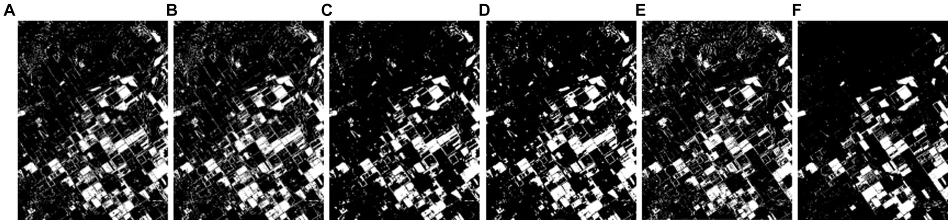
Figure 7. Change maps detected by the algorithms on the Santa Barbara dataset. (A) OSTU, (B) FCM, (C) IR-MAD, (D) FLICM, (E) MRF, (F) FLRaMF.

Additionally, upon analyzing the change result maps, it is evident that the proposed algorithm performs well in the detection of mountainous areas, exhibiting no false detections in this region and demonstrating excellent background suppression. This is attributed to the selection of the low-rank component of hyperspectral data for spectral feature extraction, effectively filtering out noise and providing support for change area determination, resulting in fewer false detections or isolated noise.

To quantitatively analyze the algorithm proposed in this chapter, the overall error (OE), precision (PCC), and Kappa coefficient of the proposed algorithm and the comparative algorithms on the Santa Barbara dataset are presented (Table 3).

Table 3

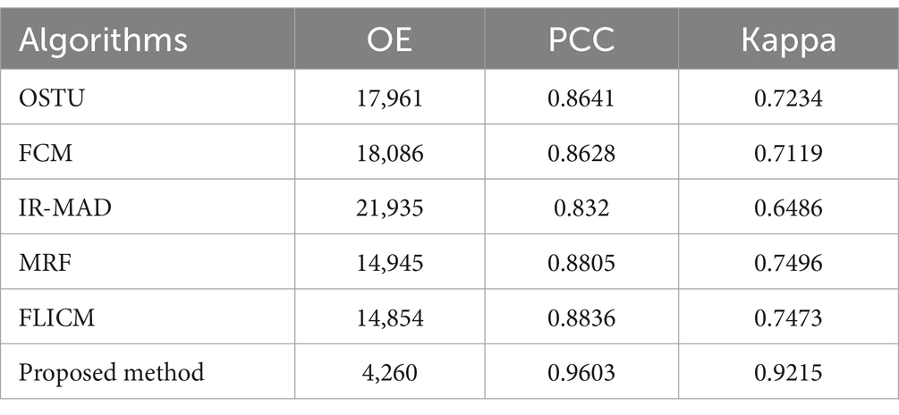
Table 3. Accuracy evaluation of Santa Barbara dataset change detection.

From the data in the table, it is evident that the proposed FLRaMF algorithm has the lowest overall error and the highest accuracy. This aligns with the observations made from the change result maps. FLICM method and MRF method follow closely in accuracy, confirming that effective utilization of spatial neighborhood information enhances the accuracy of final change information extraction when performing hyperspectral remote sensing change detection.

The high accuracy of the proposed algorithm is mainly attributed to its ability to extract change information from complex terrains in mountainous areas without false detections, a situation encountered by other algorithms to varying degrees. The proposed algorithm’s resilience to isolated noise points in complex terrains is achieved through the spatial constraints imposed by the attribute profile and the enhancement of dataset background quality through low-rank information extraction, mitigating the occurrence of noise points. Thus, the proposed algorithm achieves high accuracy on the Santa Barbara dataset, further confirming its effectiveness and demonstrating its interference resistance in complex terrain conditions.

Analyzing the change result maps obtained from various hyperspectral remote sensing image change detection algorithms on the Hermiston dataset are shown (Figure 8), it is evident that the structure of the extracted change information is pronounced in all algorithms. The main reason for this phenomenon is the limited variety of land cover types in the Hermiston dataset, with the primary focus of change information extraction being the agricultural areas. Consequently, the structure features in the change result maps are more apparent.

Figure 8

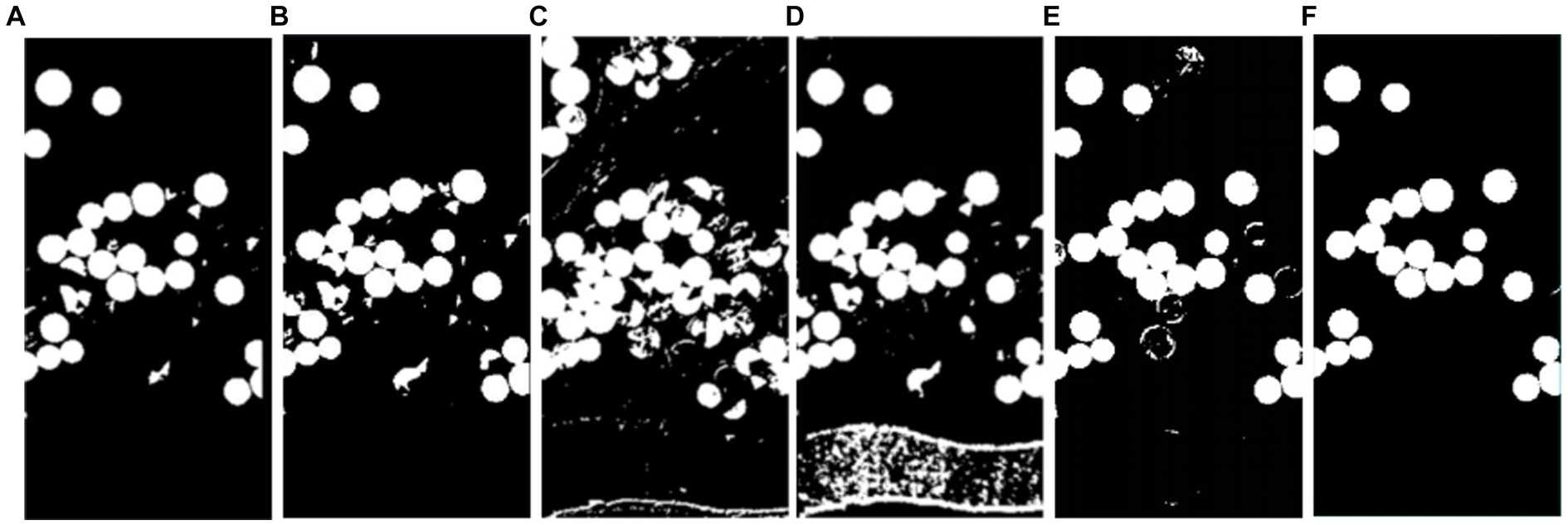
Figure 8. Change maps detected by the algorithms on the Hermiston dataset. (A) OSTU, (B) FCM, (C) IR-MAD, (D) FLICM, (E) MRF, (F) FLRaMF.

Upon observation, it can be noted that the OSTU threshold method, FCM method, and IR-MAD method exhibit a higher occurrence of isolated noise points in the change result maps. In contrast, other algorithms, including the proposed algorithm in this chapter, do not exhibit this phenomenon. The primary reason is that, in certain change areas, although they are categorized as change regions, the difference values in those areas may not be completely uniform. Therefore, using a single-threshold approach in the process of change information extraction may misclassify some pixels with difference values near the segmentation threshold as unchanged pixels, leading to the observed phenomenon.

Comparing the change result maps of the proposed algorithm with those of other algorithms, it is observed that other algorithms have more false detection areas, particularly marking some unchanged agricultural regions as change areas. This significantly impacts the accuracy of change detection.

To quantitatively analyze the algorithm proposed in this chapter, the overall error (OE), precision (PCC), and Kappa coefficient of the proposed algorithm and the comparative algorithms on the Hermiston dataset are presented (Table 4).

Table 4

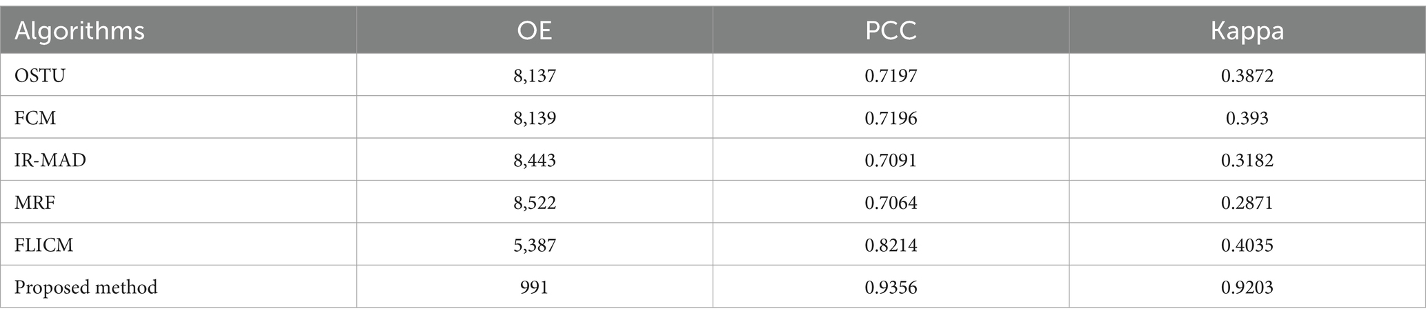
Table 4. Accuracy evaluation of Hermiston dataset change detection.

Analyzing the data in the table reveals that the proposed algorithm in this paper has the smallest overall error and the highest accuracy. The accuracy of other comparative algorithms is generally around 70%, while the accuracy of the proposed algorithm in this chapter is 93.56%, significantly higher than other algorithms.

Analyzing the change result maps obtained from various hyperspectral remote sensing image change detection algorithms on the Farmland dataset, it can be observed that the embankments between fields contribute significantly to errors. This phenomenon is particularly evident in the results of the OSTU, IR-MAD, and FLICM algorithms, while it is not observed in the detection results of the proposed FLRaMF algorithm (Figure 9). This is mainly due to the morphological constraints imposed by the attribute profile on the change targets. Additionally, the isolated noise phenomenon is more pronounced in the comparative algorithms selected in this study, while the proposed algorithm exhibits relatively minimal isolated noise. This is attributed to the optimization of the low-rank matrix for the background of the change dataset, eliminating noise interference and better distinguishing changed and unchanged pixels.

Figure 9

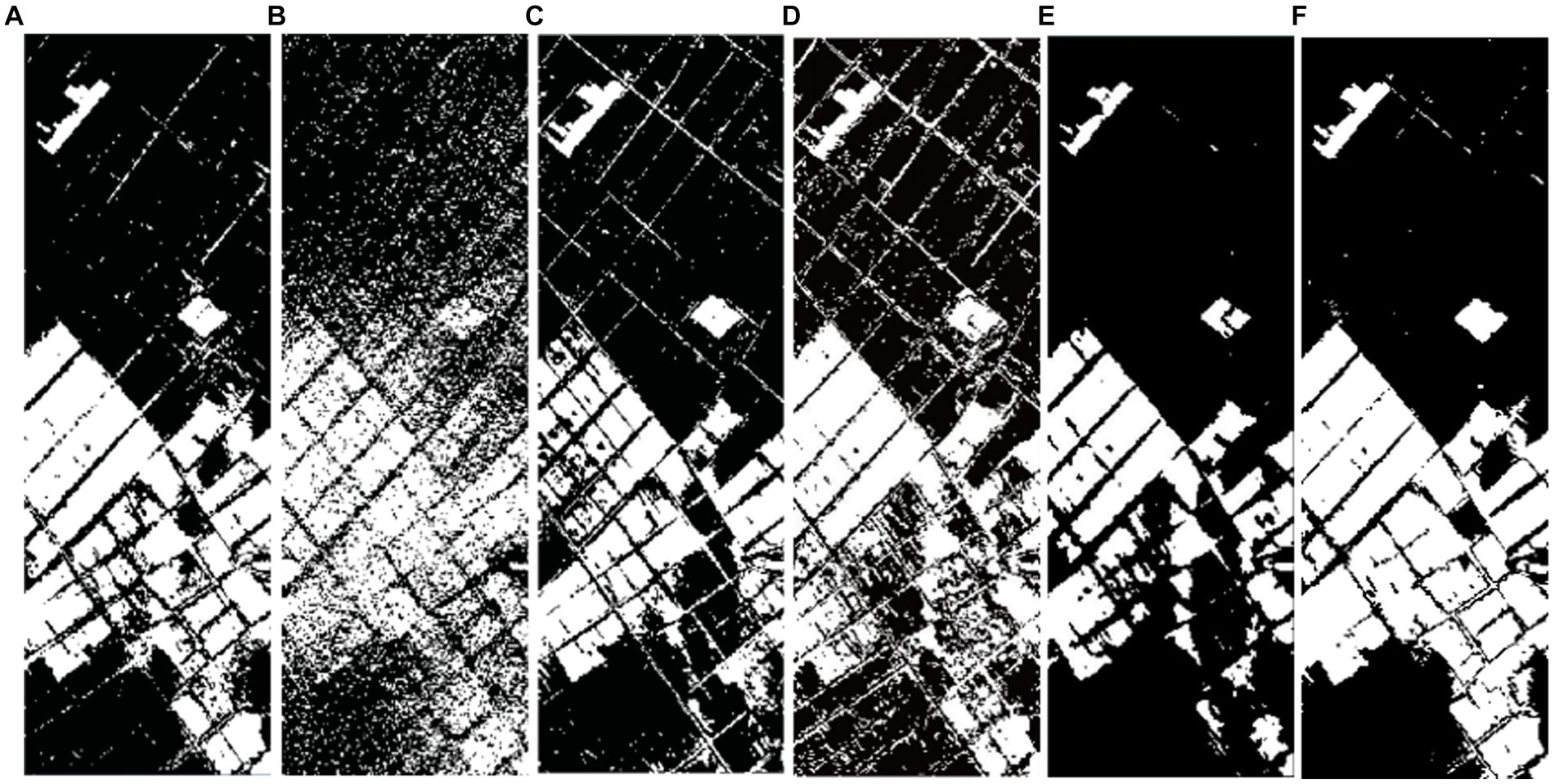
Figure 9. Change maps detected by the algorithms on the Farmland dataset. (A) OSTU, (B) FCM, (C) IR-MAD, (D) FLICM, (E) MRF, (F) FLRaMF.

Analyzing the data reveals that the proposed algorithm in this paper has the smallest overall error and the highest accuracy. The accuracy of other comparative algorithms is generally around 70%, while the accuracy of the proposed algorithm in this chapter is 88.56%, significantly higher than other algorithms (Table 5).

Table 5

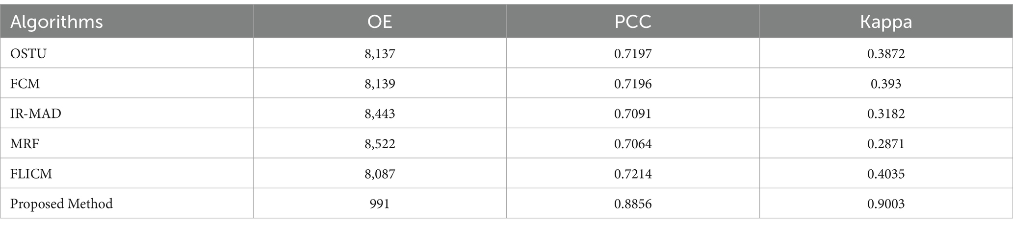
Table 5. Accuracy evaluation of Farmland dataset change detection.

3.2 Algorithm runtime performance

To comprehensively analyze the algorithms from the perspective of efficiency, this section conducted a comparative study of the runtime of each algorithm. The runtime of each algorithm on four datasets is presented (Table 6).

Table 6

Table 6. Running times of each algorithm for five datasets.

It can be observed that the runtime of the proposed FLRaMF algorithm in this paper is second only to OSTU on the four datasets, but shorter compared to FCM, IR-MAD, MRF, and FLICM methods. This is mainly attributed to the adoption of a greedy bilateral smoothing approach, aimed at reducing the time cost of singular value decomposition in each iteration during the conventional low-rank matrix extraction process. Furthermore, the method proposed in this paper provides higher accuracy compared to the comparative algorithms.

3.3 Parameter setting considerations

The FLRaMF algorithm has two crucial parameters: the rank used in the spectral domain features and the area used in the spatial domain features. For other adjustable parameters, the same default settings were used in all experiments in this paper.

Rank is one of the most critical parameters. In this section, an experiment was designed to investigate the variation of precision value AUC with the rank value (r) and the soft threshold ($\lambda$), as shown Clearly (Figure 10), with the increase of the rank value, the overall accuracy of the detection task decreases. It is generally believed that the rank value ($r$) is positively correlated with the complexity of the scene to be detected, and the changes in crops exhibit clear patterns influenced by human habits. Therefore, the default parameter setting (rank = 1) is typically sufficient to achieve the highest accuracy in completing the detection task.

Figure 10

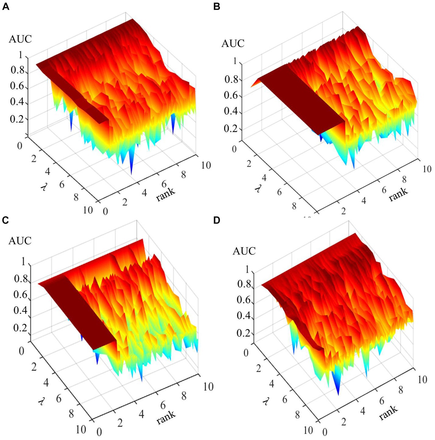
Figure 10. AUC values of FLRaMF according to changes in$\lambda$and rank$r$: (A) Bay Area, (B) Santa Barbara, (C) Hermiston, (D) Farmland.

The attribute profile’s area attribute is another key parameter. We consider 350 as the default value and observe minimal changes in accuracy within its longer intervals (Figure 10). Therefore, when performing crop change detection tasks, using the default parameter (a = 350) typically achieves the highest accuracy.

In summary, the FLRaMF algorithm proposed in this paper has relatively simple and easily understandable parameters. Particularly for crop detection, the task can often be accomplished with high accuracy using the original default parameters.

4 Conclusion

This paper introduces a fast hyperspectral change detection method for crops based on low-rank matrix and morphological feature extraction, named FLRaMF. The aim is to enhance the accuracy of crop change detection tasks, simplify usage conditions, and improve operational efficiency in unsupervised scenarios. Through greedy bilateral smoothing, noise is efficiently removed in the spectral domain to separate changing and non-changing pixels with high efficiency. Simultaneously, attribute profiles are employed to extract hyperspectral morphological features, suppressing spectral anomalies. Experimental verification on the Bay Area dataset, Santa Barbara dataset, Hermiston dataset, and Farmland dataset demonstrates the effectiveness and efficiency of this change detection method. Optimization and analysis of parameters yield default values for two crucial parameters in crop change detection. In conclusion, the FLRaMF algorithm provides a non-supervised, simple-parameter, high-accuracy, and fast-working mode for crop change detection.

In the future, we will concentrate on addressing agricultural change detection tasks covering larger areas or featuring a higher proportion of changing pixels. We are dedicated to enhancing their accuracy, applicability, and user-friendliness.

Data availability statement

The raw data supporting the conclusions of this article will be made available by the authors, without undue reservation.

Author contributions

JW: Formal analysis, Methodology, Software, Validation, Visualization, Writing – original draft, Writing – review & editing. LZ: Funding acquisition, Supervision, Writing – review & editing. RS: Formal analysis, Funding acquisition, Methodology, Supervision, Writing – review & editing. CH: Conceptualization, Formal analysis, Funding acquisition, Supervision, Writing – review & editing. DZ: Conceptualization, Formal analysis, Funding acquisition, Writing – review & editing. SL: Methodology, Software, Validation, Writing – review & editing. YL: Formal analysis, Supervision, Writing – review & editing.

Funding

The author (s) declare financial support was received for the research, authorship, and/or publication of this article. This research was supported by grants from Key Research Program of Frontier Sciences, CAS (ZDBS-LY-DQC012), China Postdoctoral Science Foundation (2022M723222), the Key Project of Research and Development of Ningxia, China (2022BEG03050), and Ministry of Education Humanities and Social Sciences Research Project (23YJAZH086).

Acknowledgments

The authors wish to thank the editors and reviewers for their valuable comments and suggestions.

Conflict of interest

SL was employed by China Siwei Surveying and Mapping Technology Company Limited.

The remaining authors declare that the research was conducted in the absence of any commercial or financial relationships that could be construed as a potential conflict of interest.

Publisher’s note

All claims expressed in this article are solely those of the authors and do not necessarily represent those of their affiliated organizations, or those of the publisher, the editors and the reviewers. Any product that may be evaluated in this article, or claim that may be made by its manufacturer, is not guaranteed or endorsed by the publisher.

References

Bosilj, P., Duckett, T., and Cielniak, G. (2018). Analysis of morphology-based features for classification of crop and weeds in precision agriculture. IEEE Robot Autom Lett 3, 2950–2956. doi: 10.1109/LRA.2018.2848305

Crossref Full Text | Google Scholar

Bouwmans, T., Aybat, N. S., and Zahzah, E. (2016). Handbook of robust low-rank and sparse matrix decomposition: Applications in image and video processing. New York: CRC Press.

Google Scholar

Bovolo, F., Bruzzone, L., and Marconcini, M. (2008). A novel approach to unsupervised change detection based on a semisupervised svm and a similarity measure. IEEE Trans. Geosci. Remote Sens. 46, 2070–2082. doi: 10.1109/TGRS.2008.916643

Crossref Full Text | Google Scholar

Dalla Mura, M., Atli Benediktsson, J., Waske, B., and Bruzzone, L. (2010). Extended profiles with morphological attribute filters for the analysis of hyperspectral data. Int. J. Remote Sens. 31, 5975–5991. doi: 10.1080/01431161.2010.512425

Crossref Full Text | Google Scholar

Demir, B., Bovolo, F., and Bruzzone, L. (2012). Detection of land-cover transitions in multitemporal remote sensing images with active. IEEE Trans. Geosci. Remote Sens. 50, 1930–1941. doi: 10.1109/TGRS.2011.2168534

Crossref Full Text | Google Scholar

Du, P., Liu, S., Gamba, P., Tan, K., and Xia, J. (2012). Fusion of difference images for change detection over urban areas. IEEE J Sel Top Appl Earth Obs Remote Sens 5, 1076–1086. doi: 10.1109/JSTARS.2012.2200879

Crossref Full Text | Google Scholar

Eismann, M. T., Meola, J., and Hardie, R. C. (2007). Hyperspectral change detection in the presenceof diurnal and seasonal variations. IEEE Trans. Geosci. Remote Sens. 46, 237–249. doi: 10.1109/TGRS.2007.907973

Crossref Full Text | Google Scholar

Ertürk, A., Iordache, M., and Plaza, A. (2016). Sparse unmixing with dictionary pruning for hyperspectral change detection. IEEE J Sel Top Appl Earth Obs Remote Sens 10, 321–330. doi: 10.1109/JSTARS.2016.2606514

Crossref Full Text | Google Scholar

Gao, L., Hong, D., Yao, J., Zhang, B., Gamba, P., and Chanussot, J. (2020). Spectral superresolution of multispectral imagery with joint sparse and low-rank learning. IEEE Trans. Geosci. Remote Sens. 59, 2269–2280. doi: 10.1109/TGRS.2020.3000684

Crossref Full Text | Google Scholar

Ghamisi, P., Yokoya, N., Li, J., Liao, W., Liu, S., Plaza, J., et al. (2017). Advances in hyperspectral image and signal processing: a comprehensive overview of the state of the art. IEEE Geosci Remote Sens Mag 5, 37–78. doi: 10.1109/MGRS.2017.2762087

Crossref Full Text | Google Scholar

Ghasemian, N., and Shah-Hosseini, R. (2020). Hyperspectral multiple-change detection framework based on sparse representation and support vector data description algorithms. J. Appl. Remote. Sens. 14:14523. doi: 10.1117/1.JRS.14.014523

Crossref Full Text | Google Scholar

Hasanlou, M., and Seydi, S. T. (2018). Hyperspectral change detection: an experimental comparative study. Int. J. Remote Sens. 39, 7029–7083. doi: 10.1080/01431161.2018.1466079

Crossref Full Text | Google Scholar

Hong, D., He, W., Yokoya, N., Yao, J., Gao, L., Zhang, L., et al. (2021). Interpretable hyperspectral artificial intelligence: when nonconvex modeling meets hyperspectral remote sensing. IEEE Geosci Remote Sens Mag 9, 52–87. doi: 10.1109/MGRS.2021.3064051

Crossref Full Text | Google Scholar

Hou, Z., Li, W., Li, L., Tao, R., and Du, Q. (2021). Hyperspectral change detection based on multiple morphological profiles. IEEE Trans. Geosci. Remote Sens. 60, 1–12.

Google Scholar

Hu, M., Wu, C., Du, B., and Zhang, L. (2023). Binary change guided hyperspectral multiclass change detection. IEEE Trans. Image Process. 32, 791–806. doi: 10.1109/TIP.2022.3233187

PubMed Abstract | Crossref Full Text | Google Scholar

Huang, Y., Zhang, L., Huang, C., Qi, W., and Song, R. (2022). Parallel spectral–spatial attention network with feature redistribution loss for hyperspectral change detection. Remote Sens. (Basel) 15:246. doi: 10.3390/rs15010246

Crossref Full Text | Google Scholar

Khanday, W. A., and Kumar, K. (2016). Change detection in hyper spectral images. Asian J Technol Manage Res 6, 54–60.

Google Scholar

Li, C., Ma, Y., Mei, X., Liu, C., and Ma, J. (2016). Hyperspectral image classification with robust sparse representation. IEEE Geosci. Remote Sens. Lett. 13, 641–645. doi: 10.1109/LGRS.2016.2532380

Crossref Full Text | Google Scholar

Li, J., Yang, B., Bai, L., Dou, H., Li, C., and Ma, L. (2023). Tfiv: multigrained token fusion for infrared and visible image via transformer. IEEE Trans. Instrum. Meas. 72, 1–14. doi: 10.1109/TIM.2023.3312755

Crossref Full Text | Google Scholar

Li, J., Zhu, J., Li, C., Chen, X., and Yang, B. (2022). Cgtf: convolution-guided transformer for infrared and visible image fusion. IEEE Trans. Instrum. Meas. 71, 1–10. doi: 10.1109/TIM.2022.3218574

Crossref Full Text | Google Scholar

Lin, Y., Li, S., Fang, L., and Ghamisi, P. (2019). Multispectral change detection with bilinear convolutional neural networks. IEEE Geosci. Remote Sens. Lett. 17, 1757–1761. doi: 10.1109/LGRS.2019.2953754

Crossref Full Text | Google Scholar

Liu, S., Bruzzone, L., Bovolo, F., and Du, P. (2014). Hierarchical unsupervised change detection in multitemporal hyperspectral images. IEEE Trans. Geosci. Remote Sens. 53, 244–260. doi: 10.1109/TGRS.2014.2321277

Crossref Full Text | Google Scholar

Liu, S., Bruzzone, L., Bovolo, F., and Du, P. (2016). Unsupervised multitemporal spectral unmixing for detecting multiple changes in hyperspectral images. IEEE Trans. Geosci. Remote Sens. 54, 2733–2748. doi: 10.1109/TGRS.2015.2505183

Crossref Full Text | Google Scholar

Liu, S., Marinelli, D., Bruzzone, L., and Bovolo, F. (2019). A review of change detection in multitemporal hyperspectral images: current techniques, applications, and challenges. IEEE Geosci Remote Sens Mag 7, 140–158. doi: 10.1109/MGRS.2019.2898520

Crossref Full Text | Google Scholar

Luo, F., Zhou, T., Liu, J., Guo, T., Gong, X., and Ren, J. (2023). Multiscale diff-changed feature fusion network for hyperspectral image change detection. IEEE Trans. Geosci. Remote Sens. 61, 1–11. doi: 10.1109/TGRS.2023.3335454

Crossref Full Text | Google Scholar

Ma, T., Hu, Y., Wang, J., Beckline, M., Pang, D., Chen, L., et al. (2023). A novel vegetation index approach using sentinel-2 data and random forest algorithm for estimating forest stock volume in the helan mountains, Ningxia, China. Remote Sens. (Basel) 15:1853. doi: 10.3390/rs15071853

Crossref Full Text | Google Scholar

Ma, T., Zhang, C., Ji, L., Zuo, Z., Beckline, M., Hu, Y., et al. (2024). Development of forest aboveground biomass estimation, its problems and future solutions: a review. Ecol. Indic. 159:111653. doi: 10.1016/j.ecolind.2024.111653

Crossref Full Text | Google Scholar

Marinelli, D., Bovolo, F., and Bruzzone, L. (2019). A novel change detection method for multitemporal hyperspectral images based on binary hyperspectral change vectors. IEEE Trans. Geosci. Remote Sens. 57, 4913–4928. doi: 10.1109/TGRS.2019.2894339

Crossref Full Text | Google Scholar

Mou, L., Bruzzone, L., and Zhu, X. X. (2018). Learning spectral-spatial-temporal features via a recurrent convolutional neural network for change detection in multispectral imagery. IEEE Trans. Geosci. Remote Sens. 57, 924–935. doi: 10.1109/TGRS.2018.2863224

Crossref Full Text | Google Scholar

Nielsen, A. A., Conradsen, K., and Simpson, J. J. (1998). Multivariate alteration detection (mad) and maf postprocessing in multispectral, bitemporal image data: new approaches to change detection studies. Remote Sens. Environ. 64, 1–19. doi: 10.1016/S0034-4257(97)00162-4

Crossref Full Text | Google Scholar

Ortiz-Rivera, V., Vélez-Reyes, M., and Roysam, B. (2006). Change detection in hyperspectral imagery using temporal principal components. [Dataset]. In: Proceedings of the SPIE, Volume 6233.

Google Scholar

Peng, J., Sun, W., Li, H., Li, W., Meng, X., Ge, C., et al. (2021). Low-rank and sparse representation for hyperspectral image processing: a review. IEEE Geosci Remote Sens Mag 10, 10–43. doi: 10.1109/MGRS.2021.3075491

Crossref Full Text | Google Scholar

Pesaresi, M., and Benediktsson, J. A. (2001). A new approach for the morphological segmentation of high-resolution satellite imagery. IEEE Trans. Geosci. Remote Sens. 39, 309–320. doi: 10.1109/36.905239

Crossref Full Text | Google Scholar

Ren, L., Hong, D., Gao, L., Sun, X., Huang, M., and Chanussot, J. (2023). Orthogonal subspace unmixing to address spectral variability for hyperspectral image. IEEE Trans. Geosci. Remote Sens. 61, 1–13. doi: 10.1109/TGRS.2023.3236471

Crossref Full Text | Google Scholar

Seydi, S. T., and Hasanlou, M. (2021). A new structure for binary and multiple hyperspectral change detection based on spectral unmixing and convolutional neural network. Measurement 186:110137. doi: 10.1016/j.measurement.2021.110137

Crossref Full Text | Google Scholar

Seydi, S. T., Shah-Hosseini, R., and Hasanlou, M. (2021). New framework for hyperspectral change detection based on multi-level spectral unmixing. Appl. Geomat. 13, 763–780. doi: 10.1007/s12518-021-00385-0

Crossref Full Text | Google Scholar

Song, A., Choi, J., Han, Y., and Kim, Y. (2018). Change detection in hyperspectral images using recurrent 3d fully convolutional networks. Remote Sens. (Basel) 10:1827. doi: 10.3390/rs10111827

Crossref Full Text | Google Scholar

Song, R., Ni, W., Cheng, W., and Wang, X. (2022). Csanet: cross-temporal interaction symmetric attention network for hyperspectral image change detection. IEEE Geosci. Remote Sens. Lett. 19, 1–5. doi: 10.1109/LGRS.2022.3179134

Crossref Full Text | Google Scholar

Vali, A., Comai, S., and Matteucci, M. (2020). Deep learning for land use and land cover classification based on hyperspectral and multispectral earth observation data: a review. Remote Sens. (Basel) 12:2495. doi: 10.3390/rs12152495

Crossref Full Text | Google Scholar

Wang, X., Ni, W., Feng, Y., and Song, L. (2023). Agf 2 net: attention-guided feature fusion network for multi-temporal hyperspectral image change detection. IEEE Geosci. Remote Sens. Lett. 20:469. doi: 10.1109/LGRS.2023.3302469

Crossref Full Text | Google Scholar

Wang, D., Saleh, N. B., Byro, A., Zepp, R., Sahle-Demessie, E., Luxton, T. P., et al. (2022). Nano-enabled pesticides for sustainable agriculture and global food security. Nat. Nanotechnol. 17, 347–360. doi: 10.1038/s41565-022-01082-8

PubMed Abstract | Crossref Full Text | Google Scholar

Wang, Q., Yuan, Z., Du, Q., and Li, X. (2018). Getnet: a general end-to-end 2-d cnn framework for hyperspectral image change detection. IEEE Trans. Geosci. Remote Sens. 57, 3–13. doi: 10.1109/TGRS.2018.2849692

Crossref Full Text | Google Scholar

Wu, S., Bai, Y., and Chen, H. (2019). Change detection methods based on low-rank sparse representation for multi-temporal remote sensing imagery. Clust Comput 22, 9951–9966. doi: 10.1007/s10586-017-1022-1

Crossref Full Text | Google Scholar

Wu, C., Du, B., and Zhang, L. (2013). A subspace-based change detection method for hyperspectral images. IEEE J Sel Top Appl Earth Obs Remote Sens 6, 815–830. doi: 10.1109/JSTARS.2013.2241396

Crossref Full Text | Google Scholar

Wu, C., Du, B., and Zhang, L. (2018). Hyperspectral anomalous change detection based on joint sparse representation. ISPRS J. Photogramm. Remote Sens. 146, 137–150. doi: 10.1016/j.isprsjprs.2018.09.005

Crossref Full Text | Google Scholar

Xia, H., Qiao, L., Guo, Y., Ru, X., Qin, Y., Zhou, Y., et al. (2024). Enhancing phenology modeling through the integration of artificial light at night effects. Remote Sens. Environ. 303:113997. doi: 10.1016/j.rse.2024.113997

Crossref Full Text | Google Scholar

Xie, T., Li, S., and Sun, B. (2019). Hyperspectral images denoising via nonconvex regularized low-rank and sparse matrix decomposition. IEEE Trans. Image Process. 29, 44–56. doi: 10.1109/TIP.2019.2926736

Crossref Full Text | Google Scholar

Yang, B., Mao, Y., Liu, L., Liu, X., Ma, Y., and Li, J. (2023). From trained to untrained: a novel change detection framework using randomly initialized models with spatial–channel augmentation for hyperspectral images. IEEE Trans. Geosci. Remote Sens. 61, 1–14. doi: 10.1109/TGRS.2023.3262928

Crossref Full Text | Google Scholar

Zhan, T., Song, B., Sun, L., Jia, X., Wan, M., Yang, G., et al. (2020). Tdssc: a three-directions spectral–spatial convolution neural network for hyperspectral image change detection. IEEE J Sel Top Appl Earth Obs Remote Sens 14, 377–388. doi: 10.1109/JSTARS.2020.3037070

Crossref Full Text | Google Scholar

Zhang, H., He, W., Zhang, L., Shen, H., and Yuan, Q. (2013). Hyperspectral image restoration using low-rank matrix recovery. IEEE Trans. Geosci. Remote Sens. 52, 4729–4743. doi: 10.1109/TGRS.2013.2284280

Crossref Full Text | Google Scholar

Zhang, W., and Lu, X. (2019). The spectral-spatial joint learning for change detection in multispectral imagery. Remote Sens. (Basel) 11:240. doi: 10.3390/rs11030240

Crossref Full Text | Google Scholar

Zhang, B., Sun, X., Gao, L., and Yang, L. (2011). Endmember extraction of hyperspectral remote sensing images based on the ant colony optimization (aco) algorithm. IEEE Trans. Geosci. Remote Sens. 49, 2635–2646. doi: 10.1109/TGRS.2011.2108305

Crossref Full Text | Google Scholar

Zheng, K., Gao, L., Liao, W., Hong, D., Zhang, B., Cui, X., et al. (2020). Coupled convolutional neural network with adaptive response function learning for unsupervised hyperspectral super resolution. IEEE Trans. Geosci. Remote Sens. 59, 2487–2502. doi: 10.1109/TGRS.2020.3006534

Crossref Full Text | Google Scholar

Zhou, J., Kwan, C., Ayhan, B., and Eismann, M. T. (2016). A novel cluster kernel rx algorithm for anomaly and change detection using hyperspectral images. IEEE Trans. Geosci. Remote Sens. 54, 6497–6504. doi: 10.1109/TGRS.2016.2585495

Crossref Full Text | Google Scholar

Zhou, T., and Tao, D. (2011). Godec: randomized low-rank & sparse matrix decomposition in noisy case. In: Proceedings of the 28th International Conference on Machine Learning, ICML 2011, Bellevue, Washington, USA.

Google Scholar