Ecological Niche Modeling: An Introduction for Veterinarians and Epidemiologists

Introduction

Spatial epidemiology is the branch of epidemiology that aims to understand the geographic distribution of diseases (including its causative agents, hosts, and related factors) (1, 2). Most diseases in animals are not distributed randomly across landscapes or regions. Instead, researchers can quantitatively determine specific environmental factors associated with the occurrence of disease (3, 4). Reports of the spatial location of pathogens, disease vectors, or reservoirs are becoming more abundant, high quality, and openly accessible for a series of infectious diseases. Similarly, data on environmental variables are increasing in availability and cover diverse spatial and temporal scales: from meters to continents and from days to centuries (both retrospective and predictive). For example, many datasets of soil composition and structure (5), landscape composition and structure (6), and climate and geomorphology (7–9) are freely and openly available for mapping diseases in aquatic and terrestrial ecosystems globally. These variables can be linked with disease data to reconstruct or predict the geographic distribution of environmentally (e.g., anthrax), vector-borne (e.g., Bluetongue disease), and directly transmitted diseases (e.g., rabies), which are important to veterinary medicine. These studies, however, need a basic understanding of Geographic Information Systems, spatial statistics, and a deep understanding of the biology of the disease system to be modeled.

Disease models accounting for environmental information are particularly informative to understand the spread of diseases that are undergoing range expansion, which is termed “distributional disequilibrium” in ecology (10–12). Ecological theories and methods are commonly used in spatial epidemiology to design and interpret models of conditions where infections are likely to occur, with outputs projected to geography as measures of “suitability.” Suitability has been defined as the “sum” of the effects of resource and environmental conditions on the fecundity, demography, and survivorship of populations (13). Ecological niche modeling has been the main branch of ecology employed to map disease transmission. Comprehensive reviews are available elsewhere regarding the fundamentals of ecological niche modeling for epidemiologists interested in its applications on medical geography of infectious diseases (14–16). This manuscript is an overview of the field of ecological niche modeling for veterinarians and epidemiologists and considers parasites (e.g., tapeworm) and pathogens (e.g., virus) as agents causing disease. The content of this review is a friendly introduction to more specialized literature and study cases described in more detail elsewhere (17, 18).

Models

A model is a simplification of a complex system. For example, in biomedicine, mice could be used as animal models to understand the effects of a drug in humans. In mathematics and statistics, equations can be used to simplify and summarize complex phenomena. Some mathematical models can be complex, by accounting for many details (i.e., parameters) in the disease system, while other models can be simple, accounting for just a few, key components of the system. Models can be used to reconstruct the structure or functioning of the system in question—termed descriptive models (e.g., the specific temperatures where a disease vector is found). Complementarily, models could be used to anticipate how the system would respond to determined “what-if-scenarios” —termed predictive models (e.g., the expected distribution of a disease vector under future temperature). Descriptive models are the basis and first stage for the development of predictive models.

Descriptive models are generally evaluated in terms of the capacity of the model to accurately reconstruct patterns found in the available data. Thus, evaluation metrics used to differentiate between good and bad descriptive models generally account for the amount of information lost (e.g., Akaike's information criterion) (19) (Figure 1A). Predictive models are evaluated based on their capacities to accurately predict, better than by random, new data (i.e., independent data not used during model calibration). Therefore, evaluation metrics used to differentiate between good and bad predictive models commonly measure model capacity to differentiation between actual data and random observations (e.g., p-value, sensitivity vs. specificity) (Figure 1B).

FIGURE 1

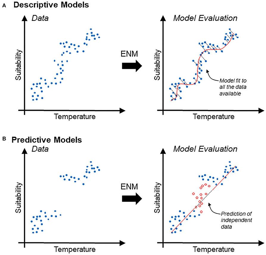
Figure 1. Schematic description of descriptive vs. predictive models in the context of ecological niche modeling. (A) Disease occurrence data (blue points) used to estimate relationships between temperature (independent variable; x-axis) and suitability (dependent variable; y-axis), interpreted as the probability of specific environmental combinations to mirror the conditions where the species actually occurs. Correlative ecological niche model (ENM) can also be based on logistic regression based on relation between continuous environmental variables and binary reports of the species (i.e., presence/absence). Note that the descriptive model (red line) is evaluated in terms of its capacity to accurately resemble the data; the information lost is expressed as the distance between the model and the data employed for model calibration (right). (B) Predictive model (same as above) intended to forecast the response of the system to an unknown status. Predictive models are generally evaluated based on their capacity to predict independent data (i.e., data not used during model calibration). Note that a predictive model could be simple (red straight line) and could result in the loss of more information. Nevertheless, independent data (red points) may be accurately predicted.

Models can also be differentiated based on their capacities of interpolation and extrapolation. Interpolation is defined as an estimation of unknown values present within the range of values from the data used to calibrate the model (20). Extrapolation is defined as the estimation of unknown values beyond the range of data used for calibration. Ideally, models aiming to be descriptive should have low interpolation and extrapolation abilities resembling good fit to the data. Predictive models are expected to interpolate and extrapolate. As a result, the final goal of the model, descriptive or predictive, should guide the design of its calibration and evaluation protocols. A perilous arena within spatial epidemiology is the development of predictive models that are evaluated using metrics developed for descriptive models or that are penalized based on extrapolation (21). Similarly, robust model evaluation of predictive models would require evaluation data statistically independent from calibration data. Thus, data-patitioning methods that do not ensure independency (e.g., cross-validation) have questionable capacity to differentiate between good and bad predictive models.

Ecological Niche Models

Previous applications of ecology to map infectious disease risk have resulted in successful disease control and prevention [e.g., (22)]. During the last two decades, valuable advancements in alternative approaches to investigate infectious diseases through applied ecology have been made (15). The ability to determine why a disease is present in one animal species, season, and geographic area but absent in others facilitates the understanding of spread and persistence of infectious diseases in wildlife and domestic animal populations, critical for veterinary medicine.

The final goal of ecological niche modeling applications in spatial epidemiology is to determine environmental conditions associated with disease occurrence. This in turn can help to identify localities where such conditions exist and that are suitable for disease introduction, maintenance, and posterior spread. These models can be conducted at the local level using accurate disease reports coupled with landscape information or at the regional level coupled with climatic variables.

Disease distributions at coarse scales are often manifested through climatic variables (e.g., temperature and precipitation) falling across expected ranges of climate values observed in the bulk of confirmed disease reports. In ecological niche theory, the fundamental niche, N_F, represents the set of abiotic environmental conditions necessary for long-term population persistence. More specifically, N_F allows population permanence without subsidy from immigration. Variables used to estimate N_F are not modified by the presence or abundance of the organism (e.g., temperature, precipitation) (14). N_F models are usually estimated at coarse-scale based on climatic signatures of biological systems to reconstruct the potential geographic distribution of organisms, revealing areas with suitable climatic conditions across broad regions (14).

Empirical and theoretical evidence from physiological experiments suggests that population growth and survival of species often have a Gaussian response to environmental gradients (23–28). That is, theory suggests that an organism's fitness responds to environmental conditions with a normal curve, where extremely low and extremely high environmental values drive low fitness, while intermediate environmental values are the optimum for fitness (Figure 2A). N_F accounts for multiple environmental variables, and when many environmental variables are considered, each with a Gaussian response curve, their combination could resemble an ellipsoid (Figure 2B). Consequently, Maguire proposed that the N_F should be convex in shape (25), with ellipsoids offering simple proxies of such convex shape (29). The Gaussian response of organisms to environmental conditions suggests that a disease reservoir or vector would have varied demographic parameters in different sections of its N_F. As a result, disease control on reservoirs or vectors (e.g., culling, vaccination) could have different effects under alternative environmental conditions. More specifically, this theory suggests that highest transmission should be expected in the optimal environmental conditions suitable for a disease reservoir or vector (30) and population health management decisions should be made accordingly.

FIGURE 2

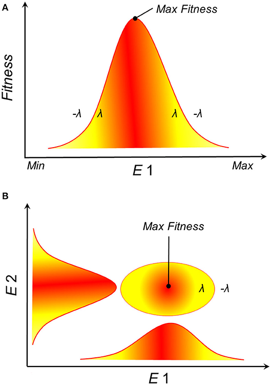
Figure 2. Theoretical representation of the fundamental ecological niche. (A) Survival or population growth (y-axis), as a proxy of suitability, shows a Gaussian response to environmental gradients (E1, x-axis). For example, population growth (λ) is positive within the environmental range tolerated by the species and negative below or above such range (–λ), with an optimum observed at intermediate environmental values (red). (B) Ellipsoidal shapes are the expected species response to n-dimensional environmental gradients. Example in a bidimensional environmental space where red is higher suitability.

Nevertheless, all the environmental conditions in N_F may not be entirely available for the species. Thus, N_F is hard to reconstruct with field data due to its theoretical nature; however, other portions of it may be more feasible to estimate. The realized niche, N_R, is the portion of the N_F that is actually occupied by the organism, reflecting fine-scale constraining effects of dispersal limitations and biotic interactions (14). Fine-scale ecological niche modeling is generally achieved by linking landscape-level variables (e.g., vegetation, host density) as a proxy of the N_R. Essentially, N_R is a close representation of the actual conditions present across the distribution of an organism. Recent experimental research shows that landscape materials (e.g., grass, wood, soil, and water) can play a role in the maintenance and spread of pathogens facilitating environmental transmission (31, 32). Satellite-derived data of vegetation phenology, soil composition, moisture, and microclimate have served as proxies of landscape features, allowing researchers to capture environmental signatures of pathogen distribution at the local level (6, 33).

Ecological niche models assume that the biotic interactions restrict species to occupy their entire N_F; therefore, that N_R is a portion of N_F (14, 34) (Figure 3). That is, maybe not all the utilizable conditions in the pathogen's N_F have the presence of the host. Additionally, ecological niche inferences must consider the geographic area accessible to the organism (termed M) and the set of environments represented across that region (14) as the limits of N_F that are available. That is, maybe not all the climates utilizable by the organism exist in the areas of study so that the existing fundamental niche, ${\text{N}}_F^{*}$, represents the portion of N_F that the species could use. ${\text{N}}_F^{*}$ is the intersection of N_F with the area accessible M, such that the existing ${\text{N}}_F^{*}$ will be a subset of N_F; any attempt to use the existing ${\text{N}}_F^{*}$ or N_R as estimates of N_F is perilous for species with limited dispersal (35). Based on this reasoning, the selection of the study area has dramatic implications on the environmental conditions to be modeled and, in turn, on estimations of N_F or N_R.

FIGURE 3

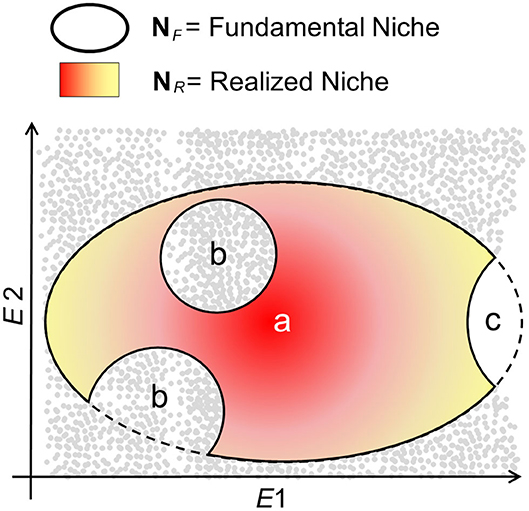
Figure 3. Schematic of N_R vs. N_F in a disease system. The fundamental niche, N_F, denotes the environmental conditions, available (gray points) or not (white), that are suitable for the organism (e.g., pathogen, vector, and reservoir) to persist and establish populations in the long term. N_F is represented as an ellipsoid with a denoting the theoretically most suitable conditions (dark red), with suitability declining to the edges of N_F (yellow). The realized niche, N_R, denotes the environments in N_F actually occupied by the organism. Nevertheless, N_R may be a subset of N_F maybe because the organism does not occupy some environments due to dispersal limitations (b), because there is not host of vector for the organism's persistence, or because the suitable environmental conditions do not exist in the area accessible (c), reducing N_F to N_F*.

The Problem of Scale in Infectious Disease Ecology

A major challenge in spatial epidemiology and distributional ecology is the identification of the scale of the analysis for a statistically correct study design and a biologically sound model interpretation. While this question may appear to be easily answered based on the data available, generally, incorrect identification of the scale may result in misleading study designs, misinterpretation of results, and inability to fill primary gaps of knowledge. Studies must identify the temporal scale (from hours and days to decades and millennia, including past, present, and future time) and the spatial scale (from centimeters to kilometers) of interest. For example, studies could be conducted in a protected area during a season, or at the continental level across a 60-years period. It is also important to define the organismal level (from molecules and genes to populations and biomes) upon which the study is focused (36). Because infectious diseases can be examined on a wide scale, from micro to macro, assumptions, data, and model interpretation will vary across scales (Figure 4).

FIGURE 4

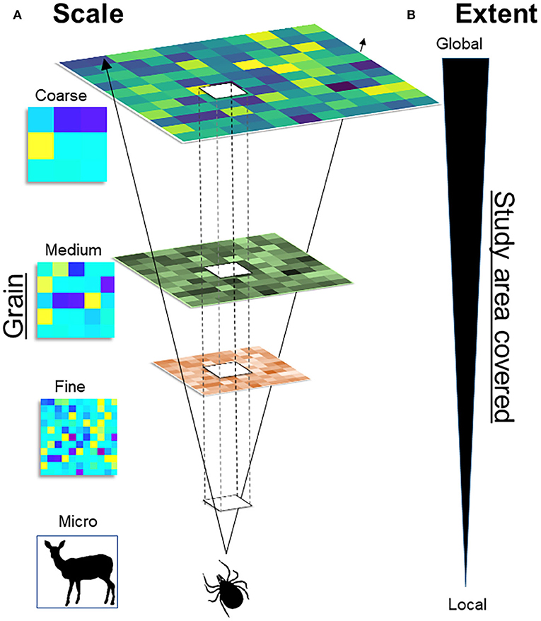
Figure 4. Multiscale framework. (A) Scale: Scale of variables (i.e., temporal and spatial) varies from the micro, to the fine, to the coarse. For example, ticks could be studied at the micro scale, by assessing its distribution across the skin of the host (e.g., deer). (B) Extent: Represents the size of the study area, from the local to the global extent. For example, increasing the extent will allow to study ticks across a forest (local) or across a continent (global). The scale and the extent are correlated: Fine-scale studies provide high detail (fine grain) but cover small study areas, coarse-scale studies cover large areas at the cost of detail (large grain).

A main assumption in epidemiology is that diseases do not occur randomly, which can be used to assess the distribution of pathogens across taxa and geographies to identify specific patterns that can be modeled and predicted. At the fine scale, models can estimate the likelihood that specific wildlife species will be suitable for vector infestation. At the medium scale, models can assess the landscape drivers of disease transmission. At the coarse scale, models could be used to reconstruct spatial patterns of the extent, direction, and speed of disease spread across continents (Figure 4).

Fine-scale studies are conducted locally and capture individual-level details in short periods of time (e.g., a season). The resources and effort necessary to conduct fine-scale research restrict their development to small study areas (e.g., a forest). Coarse-scale studies, however, can be conducted at large extents but generally fail to capture the details necessary to understand local-level phenomena. The level of detail or grain of variables quantified is linked to the scale, extent, and their capacity of prediction. Coarse-scale studies may lack details but would provide predictions that are more robust across space and time. Thus, the problem of scale in disease ecology is how predictions change as scales change (Figure 5). The problem of scale (i.e., temporal or spatial) has been described in detail by Simon A. Levin (36) and provides opportunities to better understand disease systems across space and time. Interestingly, spatial epidemiology of animal diseases seems to be biased toward local-level studies, with limited research conducted at coarser scales (37).

FIGURE 5

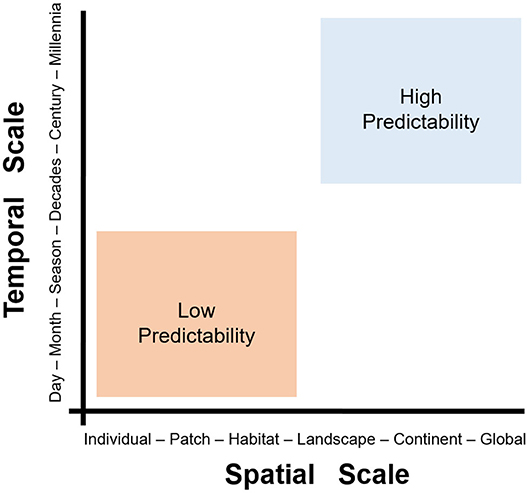
Figure 5. The problem of scale in disease ecology. Scale can be defined in two dimensions: spatial (x-axis) and temporal (y-axis). Fine-scale studies (e.g., data from at the individual-level during hours to days) can provide high-quality data and a good understanding of phenomena. The figure shows a pragmatic categorization of two spatiotemporal scales, fine (orange) and coarse (blue). Fine-scale studies (orange) tend to offer limited predictability but high detail, while coarse-scale studies (blue) offer high predictive potential at the cost of losing detail. Note that landscape/seasonal studies are somewhere in-between fine- and coarse-scale studies. Modified from Levin (36).

The organismal level is a major challenge in spatial epidemiology. For instance, the complex transmission cycles of vector-borne, water-borne, or directly transmitted diseases require two (e.g., pathogen and host) or more (e.g., pathogen, multiple vectors, multiple reservoirs, or hosts) species to be included in the model. Often in practice, modelers use a single organism to reconstruct areas of transmission, which could focus on the vector or the pathogen. While a parsimonious approach, it requires a strong understanding of the ecology of the disease in question to identify the organism that best explains the disease system. Thus, a next frontier in ecological niche modeling applications to disease systems is the inclusion of more biological components of the cycle of transmission in the modeling process.

Ecological Niche Modeling and Spatial Epidemiology

Ecological niche modeling has proven to be a useful tool for forecasting distributions and distributional changes for a vast number of organisms (22, 38, 39) and is increasingly employed to predict distributions of pathogens on diverse spatial scales (15). Traditional ecological niche modeling frameworks, however, may make unrealistic assumptions and therefore yield inaccurate predictions. These modeling frameworks must therefore be revised and amended if they are to work in epidemiology (40). Ecological niche modeling estimates ecological niches of species by linking spatial occurrence records with environmental covariates, via correlative or mechanistic approaches (41, 42). Theory and analytical approaches of ecological niches have been described during the last century (43), especially for biodiversity and conservation studies.

A decade ago, it was hypothesized that coarse-scale geographic distributions of species were constrained principally by abiotic environmental conditions (i.e., inert variables) across relevant regions, with biotic interactions having negligible effect [termed the Eltonian Noise Hypothesis (14, 29)]. As a result, most modelers have considered it reasonable to assume that influences of biotic interactions could be neglected in ecological niche modeling (29). The Eltonian Noise Hypothesis, however, was conceived in the context of free-living organisms (e.g., plants, birds). Currently, most ecological niche modeling applications do not include biotic variables (i.e., derived from living organisms). Epidemiologists of infectious disease and veterinarians have a clear understanding of the major flaws of models neglecting biotic interactions because infectious diseases are by definition biotic interactions.

Developing models based solely on abiotic variables make model outputs of easy interpretation. For example, a model based on pH and humidity could generate estimates of suitability with regard to environmental conditions. Nevertheless, the role of biotic variables has not been assessed rigorously in parallel analyses in disease ecology [but see (44)]. Indeed, incorporation of biotic variables in ecological niche modeling analyses for diseases was proposed only relatively recently (45), and such applications remain rare in spatial epidemiology. The inclusion criteria of the biotic variables to be used, their temporal and spatial scales, and whether biotic variables should be used before, during, or after the model calibration process remain understudied (40). Currently, use of abiotic-only predictors (e.g., climate) dominates the literature regarding modeling and predicting geographic distributions of pathogens. Including biotic variables in the ecological niche modeling process would require a detailed and a priori definition of the modeling outputs. For example, a model including host density or percentage of vaccination coverage would require a revision of the “suitability” term in the context of each study (e.g., suitability for transmission or exposure); alternatively, other terms would need to be employed for modeling disease systems, such as risk (46) or relative occurrence rate (47). Understanding the role of biotic variables in ecological niche modeling may revolutionize the utility of these tools drawn from ecology for disease risk mapping.

Ingredients to Make an Ecological Niche Model

Historically, “ingredients” to build ecological niche models have been summarized in three major categories: occurrence data, environmental data (abiotic or biotic variables), and algorithm (Figure 6). Occurrence data are represented as disease cases, or serology or direct detection of pathogens or parasites, or records of vectors, intermediate hosts, or reservoirs recorded geographically as coordinates (i.e., latitude and longitude). Environmental data are represented at coarse (i.e., climate) and fine (e.g., vegetation indices) resolutions in terms of the abiotic and biotic environmental conditions where occurrence data are collected. Then, to link environmental conditions and disease occurrence, correlative or classification algorithms are generally used. This analytical framework has been criticized due to the limited understanding of the user regarding the potential data and algorithm limitations, and the theoretical bases of the algorithm employed (48). Careless applications of this simple modeling framework has been termed “click-and-run ecological niche modeling” (49) and has resulted in misleading ecological niche modeling applications (50–52). Indeed, studies to reconstruct disease distributions should avoid using protocols and parameterization scenarios developed for other taxa, regions, or periods. Instead, the modeling protocol for disease mapping should be specific to the study question, data available, and assumptions of the disease system.

FIGURE 6

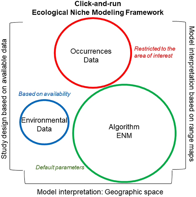
Figure 6. Click-and-run ecological niche modeling framework. This modeling framework is data-driven, with uncaring study designs. Syndromes used in identifying click-and-run ecological niche models include (i) strong emphasis on the good performance of the algorithm employed based on external literature and use of default parameters (green), (ii) moderate emphasis on the quality and quantity of the disease localities (i.e., occurrence data; red), with limited data curation and evaluation, and (iii) little or no justification and defense of the environmental variables selected for model calibration (blue). Additionally, these models generally fail to define the ecological niche to be estimated, N_F vs. N_R. The study area of these models is generally delimited based on data availability or administrative boundaries, while model interpretation is generally based on visual inspection of maps. Circle size denotes magnitude of importance assigned to each category.

The click-and-run modeling framework (Figure 6) is based on the use of “recipes” to model the distribution of any species, neglecting the biology of the organism in question. These models also neglect biases or artifacts in the data used for model calibration and the functionality of the algorithm employed. This approach requires limited data curation and model parameterization and was used in the past for single-species ecological niche models, but is currently used for studies modeling hundreds or thousands of species to capture coarse ecological patterns (i.e., macroecology). Model evaluation in click-and-run modeling is generally poor or absent, making this modeling framework particularly questionable when modeling infectious diseases.

Models should include occurrence data curated carefully to include only trusted occurrence records for model calibration. Trustworthy disease occurrence records should have traceable diagnostic methods, data sources, transparent surveillance protocols, temporal details, and quantified uncertainty (e.g., spatially error, sensitivity of the diagnostic method). That is, selection of the occurrence data should include an exhaustive inspection of the metadata to reduce errors followed by estimations and mitigations of duplicates, autocorrelation, and sampling bias, supported by detailed protocols as described by Cobos et al. (53).

Ecological niche modeling of disease systems should consider abiotic environmental variables (e.g., temperature, soil, precipitation) that fit the scale of interest and the biology of the disease to be modeled. For example, historical satellite-derived bioclimatic data can be employed at a pixel resolution of 20 km, if this is in agreement with the approximate home range size of a pathogen's reservoir (~10 km) (10). In this case, one could use land surface temperature (°C) and ground humidity (kg) to overcome limitations of interpolated climatic data (8). That is, it has been found that satellite-derived data overcome limitations of the original interpolations found in the climatic data from ground stations (54). For example, WorldClim, a commonly used resource for climate data, often includes only 0.001% of empirical data and 99.99% of interpolated data, resulting in high spatial lag (autocorrelation) and frequent aberrant and unrealistic climatic values (15).

Biotic variables (e.g., host density, prey density, and predator occupancy) are biological factors shaping the distribution of a species or disease at the local level (55, 56). Biotic variables must be selected on the basis of the natural history of the target pathogen, including the presence or abundance of other organisms that facilitate or limit its presence. For some pathogens, relevant positive biotic factors that facilitate the presence of disease may include co-infections with other pathogens, vegetation preferences of vectors, and host availability, behavior, and density. Negative biotic factors that limit pathogen circulation and establishment may include host immunity and biodiversity values (40, 46, 57). Biotic components may be critical to understand the ecology of pathogen transmission, and their effects are evident when developing studies at fine geographic scales (46), although the question of their action across broad geographic extents remains unanswered. Nevertheless, based on the biology of the pathogen, biotic variables could include proxies of host availability (58), anthropogenic disturbance (59), wildlife reservoirs availability (60), and barriers of disease spread (61, 62). Each of these dimensions has been found to be predictors of infectious diseases (10, 45, 63–67).

The inclusion of biotic variables in ecological niche modeling could be done before, during, and after the calibration of the model. For example, biotic variables could be used before the development of the model by restricting the distribution of the focal species (e.g., pathogen) to regions where biotic interactions may occur (e.g., host distribution; pre-processing). Biotic variables could be added to model calibration by incorporating biotic factors as predictor variables in the ecological niche modeling (e.g., host density; processing). Alternatively, biotic variables could be used once the model is developed by incorporating biotic variables on the final model output (post-processing). For example, a hypothetical model to estimate transmission risk of rabies (Lyssavirus) transmitted by vampire bats (Desmodus rotundus) at the local level could include the use of abiotic (e.g., temperature and precipitation) and biotic variables. Biotic variables could include livestock densities as proxy for food resources for the vampire bats (58), surface of roads as proxy of local-scale barriers (61, 62), and satellite-derived nighttime light surface as proxy of populated centers (59), since these variables have been proposed as predictors of rabies in wildlife (10, 63–67). That is, when biotic variables are included to reconstruct a disease system, it is crucial to identify key factors that directly facilitate or limit transmission. Using biotic variables in ecological niche modeling is still not a common practice and more research is necessary in this area to develop a revised modeling framework.

A revised ecological niche modeling framework could facilitate replicable estimations for any disease system (Figure 7). Nevertheless, each component of a revised modeling framework (i.e., occurrences, environmental variables, and modeling algorithm) would require careful inspection to discard noise signals due to incorrect study designs. That is, study designs should be based on biologically justifiable study areas and variables, which are important drivers of ecological niche modeling performance. In some situations, the protocol will allow one to determine if a robust ecological niche model is feasible or not.

FIGURE 7

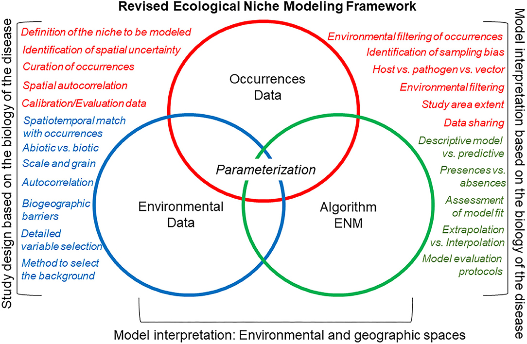
Figure 7. Canonical ecological niche modeling framework (a.k.a. “Peterson's Framework”). This revised ecological niche modeling framework includes some of the critical decisions necessary to develop a comprehensive, replicable ecological niche model that accounts for the natural history of the organism, the quality of the data, and the goal of the model. Here, occurrence data (red), environmental data (green), and the integrative algorithm (blue) have comparable importance regarding their assessment during the modeling process (i.e., same size of circles). The main differences of this canonical ecological niche modeling framework, as compared with the classic ecological niche modeling framework (Figure 6), are that more details are evaluated for each modeling component (circles), model design, and interpretation account for the ecology of the organism and data available, and that model outputs are interpreted in geographic and environmental dimensions.

An important component of the revised protocol is the careful inspection of occurrences using a specified inclusion criterion that prioritizes quality over quantity. To assess and mitigate sampling bias in disease reports, modelers can use the method proposed by Varela et al. (68), which compares models from different occurrences filtering methods to mitigate both oversampled areas and oversampled environments. This approach allows the generation of a series of models under different bias mitigation scenarios to (i) reduce model overfitting (i.e., models mirroring closely the data, resulting on limited learning from the model compared with the raw data) and (ii) capture variability for more informed model interpretations. This methodology has been employed broadly to study the distribution of biodiversity but has been barely used to model infectious diseases. In the revised protocol (Figure 7), model calibration could include biotic variables as predictor (45, 69). Nevertheless, researchers must clarify the units and interpretation of the modeling output.

Finally, the study area of interest [M sensu (70)] is a major component of the modeling process. A common failure in ecological niche modeling applications based on correlative models is to pragmatically determine the study area. Restricting models based on administrative areas (e.g., municipality, department, province, and state) does not account for the biology of the organism. Pathogens do not know about political borders; therefore, models should account for biogeographic barriers (e.g., rivers, roads, impervious surfaces, and oceans) for biologically sound study designs.

The perils of careless study-area delimitations will result in models that are misaligned with the primary question of the study, the ecology of the organism, resulting in underestimations of the true potential of the disease spread. For example, the mosquitoes Aedes aegypti and Ae. albopictus are important vectors of many arboviruses, including Zika, Dengue, and Chikungunya viruses with transmission reported globally. Nevertheless, one may be interested in modeling the distributional ecology of these mosquitoes in a specific study area (Figure 8A). For example, mosquito presence in Guatemala along with climate information from the sampling region will only capture environmental tolerances of the species in that particular area. This may therefore result in a gross underestimation of the true potential distribution of the vectors and the diseases they transmit. Indeed, these mosquito species are ecological generalist species that tolerate a broad range of climatic conditions and have global distributions (Figures 8B,C). Thus, real tolerances and actual potential distribution of species could be masked by a restricted study area that only accounts for a portion of the species truly potential.

FIGURE 8

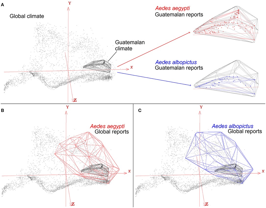
Figure 8. Effects of study area M on ecological niche modeling results. An example of an ecological niche model of arbovirus vectors Aedes aegypti (red) and Ae. albopictus (blue), which occur worldwide, to predict transmission risk in Guatemala. Global climate data (gray dots) show the broad range and diversity of global environmental conditions summarized in the first three components of bioclimatic variables (red axis). Restricting the study to Guatemala (gray polyhedron) will require to use species records only across this country (red and blue dots), resulting in a subset of occurrence records, and environmental tolerances, of the mosquito species (red and blue polyhedrons) (A). Accounting for all the available data for the vector species, however, reveals that Guatemala only contains a portion of the species environmental tolerances (B,C). As a result, when the study design is restricted to Guatemala as the study area M, and to its climate and environmental space, the model would yield in an incomplete reconstruction of the actual distributional potential of vector-borne diseases. Restricting the models to Guatemala would require other, fine-scale, landscape-level environmental variables. Otherwise, models will simply mirror the density of points. Models constructed using an envelope algorithm in NicheA (71).

Ecological Niche Modeling Algorithms and Tools

Modeling algorithms in ecological niche modeling have been described elsewhere (47, 72–74), generating starting points for new modelers. Algorithms to develop ecological niche models can be divided into three categories: presence-absence, presence-background, and presence-only. Presence-absence algorithms need a set of localities where the organism occurs (i.e., presence) and a set of localities where the organisms does not occur (i.e., absence). Presence-absence models are calibrated by comparing environmental conditions where the organism is present vs. where it is absent and are generally useful to reconstruct the distribution of diseases at fine scale and short periods, resulting in the need of accurate localities and high-resolution environmental variables. These models, however, have limited capacities to be projected to different areas or periods, instead, their signals are space and time specific. Many algorithms are available including regression (e.g., Generalized Linear Models and Generalized Additive Models) (Figure 1) and classification (e.g., Boosted Regression Trees, Random Forest, and Support Vector Machines) (Figure 9A) algorithms, with protocols described in detail elsewhere (75).

FIGURE 9

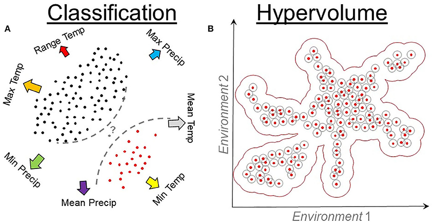
Figure 9. Classification and hypervolume models. (A) Classification algorithms require environmental values where the species is present (red points) and absent (black points). Presence and absence data are linked to environmental values (arrows) to quantify the probability (question mark) of identifying a locality (gray point) as a suitable or unsuitable. Classification algorithms use these data to inform a series of rules (dashed lines) that vary among algorithms. Temp, temperature; Precip, precipitation. (B) Hypervolume algorithms quantify the density or cluster of presence records of the organisms in environmental dimensions. Hypervolumes measure the distance (gray cycles) among occurrences (red points) in an environmental space (arrows) to determine a best-fit model (red buffer).

Occurrence data are generally robust, while absence data are largely questionable in quality and of limited availability [discussed in (14)]. To solve this problem, researchers generally “simulate” absence data to be able to use presence-absence algorithms. A common approach to simulate absence data is to generate random points across the study area. Presence-absence models that use simulated (i.e., fake) absence data during calibration are termed presence-background models. Presence-background algorithms thus use the same regression and classification algorithms used for presence-absence models, with the unique philosophical variation regarding the interpretation of absences vs. background points. Also, because the background corresponds to the study area, calibration of these algorithms is highly sensitive to variations in the extent of the study area extent selected.

Maxent is a popular ecological niche modeling algorithm based on logistic-like regressions comparing densities of occurrences (presences), densities of random points (background), and continuous environmental variables using diverse sets of parameters in the calibration process (47). Maxent protocols have been summarized in a series of software including Wallace (76), dismo (75), ENMeval (77), and KUenm (78) packages in R. Wallace is a user-friendly analytical environment to calibrate Maxent models, making it a good starting point for new users since it contains detailed instructions (76). Dismo provides less details regarding the different assumptions and complementary scientific literature, but it is a good starting point for new users interested on modeling in programming environments (75). ENMeval is essentially the programming environment of Wallace and allows more detailed parameterization and evaluation of models (77). KUenm allows detailed, reproducible ecological niche models using Maxent and provides detailed model calibration and selection not available in the other packages (78), overcoming some of the perils of niche model applications for infectious diseases regarding differentiation between good and bad models (46). The KUenm package would be an ideal choice for advanced users since parameterization and installation would require advanced programming skills.

Presence-only algorithms focus solely on the environmental values linked to each occurrence record for calibration. As a result, calibration of these modes is insensitive to changes in the extent of the study area. Classic presence-only methods include environmental envelopes, which are ellipsoids, squares, or convex-hull that surround the occurrences in an environmental space (Figure 9), with algorithms that include Bioclim (75) and NicheA (71). Emerging presence-only methods include hypervolumes estimated using estimators of density (79) and cluster of occurrences in the environmental space (80). Protocols for hypervolume estimations have been described elsewhere (34, 74), and their use is expected to become common for N_R estimations due to the automatization of their workflows and computational optimization.

Ecological Niche Modeling and Climate Change

A key set of questions in spatial epidemiology relates to effects of global change on the geographic distribution of infectious diseases and the potential of disease reservoirs or vectors to respond to such changes (81). Global change includes climate and land cover changes and the accelerated introduction of invasive species (82–84). A recent assessment proposed that catastrophic climate change effects will be perceived with even a 1.5°C annual mean temperature increase in the coming decades (85).

Ongoing climate change trends have been defined as human-induced, with unprecedented effects on biodiversity, impacting many organisms involved in disease transmission cycles (86). Climate change in the Anthropocene is generating geographic (87) and elevational (88) shifts of biodiversity, including organisms involved in disease transmission (89). Climate change is expected to produce bigger and more frequent weather events and wildfires (90, 91) and reductions of crop yields (92, 93), which together could generate ecological imbalance facilitating pathogen spillover (94). Understanding climate effects on directly transmitted diseases, however, remains in its infancy. Ecological niche models are a promising tool to help anticipate likely responses of disease systems to climate change. Recent assessments of vector-borne diseases have challenged paradigms related to climate and infectious diseases (95–97).

A recently published meta-analysis demonstrated that many popular algorithms for ecological niche modeling generally overestimate organisms' ability for adaptation to changing environments (98). The best forecasts should come from analyses of extensive data with simple algorithms (21, 99). That is, robust models require abundant, high-quality input occurrence data; these data are generally limited in availability in developing countries, so research about global change effects on diseases may be biased to developed countries (100). Nevertheless, even when data limitations may exist, ecological niche models provide opportunities to understand how global change can affect infectious diseases globally. Based on the observations described above, when limited data are available, the use of multiple algorithms could help to explain uncertainty in model estimates.

The present understanding of potential climate change effects on organisms is biased geographically to temperate-zone countries (101). Nevertheless, tropical countries already show considerable climate change manifested in just the last three decades. Hence, the tropics represent an important priority for global change disease ecology research in view of their considerable research gaps, their role in modulating global climate, the need to understand organisms' responses to environmental change beyond temperate areas, and the need to assess niche evolution empirically in more rigorous analyses (102).

The Paradox of Directly Transmitted Diseases

It is not surprising that ecological niche modeling applications in spatial epidemiology are biased toward vector-borne diseases. Data of disease vectors (e.g., fleas, mosquitoes, ticks) are broadly and openly available for many diseases and regions (103). Vectors are also highly responsive to changes in microclimate, with strong responses in their abundance, richness, distribution, and behavior linked to climate and landscape variation (104). As a consequence, ecological niche models of vector species provide good proxies of potential distributions of vector-borne diseases.

Environmentally transmitted diseases, such as anthrax, leptospirosis, and histoplasmosis, can also be studied using ecological niche modeling. Key components of the models include variables resembling the environmental drivers of parasite and pathogen persistence in the environment (e.g., humidity, temperature, and soil pH). When such variables are not available, some proxies could be used with their respective caveats.

Ecological niche models have many advantages compared with other disease modeling approaches, especially with regard to the biological bases that support the use of environmental drivers to map disease distributions. Nevertheless, ecological niche models are not suitable for the study of many disease systems, especially for studies aiming to understand direct transmission between individuals or populations. In such situations, other modeling approaches could be more appropriated (e.g., compartmental models). Similarly, ecological niche modeling may be a perilous modeling framework to use for animal disease systems where the environmental conditions are less important for transmission compared with animal density or human behavior.

Directly-transmitted diseases are more challenging to map based on environmental conditions. Many fine-scale factors (e.g., host density, age, immune status) shaping direct disease transmission may be required for correct reconstruction of transmission, but variables of such factors are generally not available. When the directly-transmitted disease includes an animal reservoir (e.g., wildlife), ecological niche models can focus on such species for the reconstruction of likely areas of transmission.

Ecological niche modeling of directly-transmitted animal diseases are a “dark side” that many veterinary epidemiologists avoid. Limited data of crucial factors associated with transmission and potential economic and ethical implications generally reduce explorations of directly-transmitted animal diseases. For example, the porcine reproductive and respiratory syndrome (PRRS, caused by a virus from the family Arteriviridae) affects the pork industry so that understanding and anticipating its distribution may have enormous benefits for its control and prevention in pig farms. Nevertheless, intensive farms may have controlled environmental conditions, so that the environmental conditions inside the pig farms may not reflect the surrounding climatic conditions. Thus, ecological niche modeling of PRRS risk based solely on the surrounding climate of farms is analytically and computationally feasible [e.g., (105, 106)], but such models will provide an erroneous signals of the environmental conditions suitable for transmission. That is, even when one can model linkages between climate and reports of directly-transmitted diseases, such models could be incomplete, biased, or misleading, and local factors may be more important (107). Paradoxically, models of directly-transmitted diseases are still popular.

Conclusion

Spatial epidemiology of animal diseases seems to be dominated by local-level studies (37). Thus, ecological niche modeling approaches provide an opportunity to reconstruct environmental conditions suitable for diverse animal diseases to identify areas where transmission is expected. Since disease systems need at least two organisms interacting (host and pathogen), biotic interactions may lie at the core of the pathogen's ecological niche, and neglecting interacting organisms in pathogen dynamics (i.e., maintenance, reproduction, transmission, and spread) may limit the success of forecasts. Pathogen transmission is strongly influenced by fine-scale interactions among infected and susceptible hosts, which can be further affected by host behavior and pathogen demography/transmission. Given the complexity of these interactions, traditional single-species ecological niche modeling approaches could fail to predict disease distributions and transmission risk accurately and protocols need to be revised with caution.

A new challenge in veterinary epidemiology is to avoid falling behind advances that distributional ecology offers in terms of theory and methods to map parasites, pathogens, vectors, and reservoir. This overview is by no means a detailed summary of all the advances in the field of ecological niche modeling. Instead, this review provides a brief introduction to the field facilitating a more effective use of the comprehensive ecological niche modeling courses freely available (e.g., https://www.youtube.com/watch?v=vj8qTo56rPA&ab_channel=A.TownsendPeterson) (108). Veterinary epidemiology needs more ecology, and ecologists modeling disease distributions need to incorporate health professionals for sound and biologically realistic model interpretations (15). Veterinary epidemiologists may find ecological niche modeling useful for disease control efforts, especially for infectious diseases with vectors or wildlife reservoirs. The limited presence of epidemiologists and disease ecologists in the ecological niche modeling community increases the risk of inaccurate and misleading forecasting of infectious diseases of questionable quality and usefulness for stakeholders [e.g., (109)]. The broadly available epidemiological data, collected systematically from humans, animals, and plants, can help to advance the study of disease transmission. The comprehensive understanding of disease systems by veterinarians provides unique opportunities for their active participation in the field of spatial epidemiology. Nevertheless, mature and ethical ecological niche modeling applications for disease mapping would require familiarity with classic ecological theory.

Author Contributions

The author confirms being the sole contributor of this work and has approved it for publication.

Funding

This work was supported by Virginia Tech Startup Funds for LE.

Conflict of Interest

The author declares that the research was conducted in the absence of any commercial or financial relationships that could be construed as a potential conflict of interest.

The reviewer GM declared a past co-authorship with the author LE to the handling editor.

Acknowledgments

The author thanks A. T. Peterson for his contributions to the field in the form of online and in-person training, books, and manuscripts that triggered the main ideas of the new modeling framework. Paige Van de Vuurst, Steven. N. Winter, Diego Soler-Tovar, Natalie Brown, and Emily Hardgrove provided helpful comments in a final version of the manuscript. Thanks also to Jaber Amine Belkhiria, Jörn Gethmann, and Gustavo Machado for their evaluation and suggestions. Thanks to Salome Dürr, Victoria J. Brookes, and Andres M. Perez for the invitation to contribute to this special issue.

References

1. Pfeiffer DU, Robinson TP, Stevenson M, Stevens KB, Rogers DJ, Clements ACA. Spatial Analysis in Epidemiology. Oxford: Oxford University Press (2008). doi: 10.1093/acprof:oso/9780198509882.001.0001

CrossRef Full Text | Google Scholar

2. Ostfeld RS, Glass GE, Keesing F. Spatial epidemiology: an emerging (or re-emerging) discipline. Trends Ecol Evol. (2005) 20:328–36. doi: 10.1016/j.tree.2005.03.009

PubMed Abstract | CrossRef Full Text | Google Scholar

3. Eisen RJ, Lane RS, Fritz CL, Eisen L. Spatial patterns of lyme disease risk in California based on disease incidence data and modeling of vector-tick exposure. Am J Trop Med Hyg. (2006) 75:669–76. doi: 10.4269/ajtmh.2006.75.669

PubMed Abstract | CrossRef Full Text | Google Scholar

4. Lash RR, Carroll DS, Hughes CM, Nakazawa Y, Karem K, Damon IK, et al. Effects of georeferencing effort on mapping monkeypox case distributions and transmission risk. Int J Health Geogr. (2012) 11:23. doi: 10.1186/1476-072X-11-23

PubMed Abstract | CrossRef Full Text | Google Scholar

5. Hengl T, Mendes de Jesus J, Heuvelink GBM, Ruiperez Gonzalez M, Kilibarda M, Blagotić A, et al. SoilGrids250m: Global gridded soil information based on machine learning. PLoS ONE. (2017) 12:e0169748. doi: 10.1371/journal.pone.0169748

PubMed Abstract | CrossRef Full Text | Google Scholar

6. Horning N, Robinson J, Sterling E, Turner W, Spector S. Remote Sensing for Ecology and Conservation. New York, NY: Oxford University Press (2010).

Google Scholar

7. Karger DN, Conrad O, Böhner J, Kawohl T, Kreft H, Soria-Auza RW, et al. Climatologies at high resolution for the earth's land surface areas. Sci Data. (2017) 4:1–20. doi: 10.1038/sdata.2017.122

PubMed Abstract | CrossRef Full Text

8. Vega GC, Pertierra LR, Olalla-Táraga MÁ. MERRAclim, a high-resolution global dataset of remotely sensed bioclimatic variables for ecological modelling. Sci Data. (2019) 4:170078. doi: 10.1038/sdata.2017.78

CrossRef Full Text | Google Scholar

9. Amatulli G, Domisch S, Tuanmu M-N, Parmentier B, Ranipeta A, Malczyk J, et al. A suite of global, cross-scale topographic variables for environmental and biodiversity modeling. Sci Data. (2018) 5:180040. doi: 10.1038/sdata.2018.40

PubMed Abstract | CrossRef Full Text | Google Scholar

10. Benavides JA, Valderrama W, Streicker DG. Spatial expansions and travelling waves of rabies in vampire bats. Proc R Soc B. (2016) 283:20160328. doi: 10.1098/rspb.2016.0328

CrossRef Full Text | Google Scholar

11. Hutter SE, Brugger K, Sancho Vargas VH, González R, Aguilar O, León B, et al. Rabies in Costa Rica: documentation of the surveillance program and the endemic situation from 1985 to 2014. Vector-Borne Zoonotic Dis. (2016) 16:334–41. doi: 10.1089/vbz.2015.1906

PubMed Abstract | CrossRef Full Text | Google Scholar

12. Piaggio AJ, Russell AL, Osorio IA, Jiménez Ramírez A, Fischer JW, Neuwald JL, et al. Genetic demography at the leading edge of the distribution of a rabies virus vector. Ecol Evol. (2017) 7:5343–51. doi: 10.1002/ece3.3087

PubMed Abstract | CrossRef Full Text | Google Scholar

13. Soberón J. The relationship between use and suitability of resources and its consequences to insect population size. Am Nat. (1986) 127:338–57. doi: 10.1086/284488

CrossRef Full Text | Google Scholar

14. Peterson AT, Soberón J, Pearson RG, Anderson RP, Martínez-Meyer E, Nakamura M, et al. Ecological Niches and Geographic Distributions. Princeton: Princeton University Press (2011).

Google Scholar

15. Peterson AT. Mapping Disease Transmission Risk. Baltimore: Johns Hopkins University Press. (2014).

Google Scholar

16. Araújo MB, Anderson RP, Barbosa AM, Beale CM, Dormann CF, Early R, et al. Standards for distribution models in biodiversity assessments. Sci Adv. (2019) 5:1–12. doi: 10.1126/sciadv.aat4858

CrossRef Full Text

17. Cuervo-Robayo AP, Escobar LE, Osorio-Olvera LA, Nori J, Varela S, Martinez-Meyer E, et al. Introduccion a los análisis espaciales con enfasis en los modelos de nicho ecologico. Biodivers Inform. (2017) 12:45–57. doi: 10.17161/bi.v12i0.6507

CrossRef Full Text | Google Scholar

18. Peterson AT, Anderson RP, Cobos ME, Cuahutle M, Cuervo-robayo AP, Escobar LE, et al. Curso modelado de nicho ecológico, versión 1.0. Biodivers Informatics. (2019) 14:1–7. doi: 10.17161/bi.v14i0.8189

CrossRef Full Text | Google Scholar

19. Burnham KP, Anderson DR, Huyvaert KP. AIC model selection and multimodel inference in behavioral ecology: some background, observations, and comparisons. Behav Ecol Sociobiol. (2011) 65:23–35. doi: 10.1007/s00265-010-1029-6

CrossRef Full Text | Google Scholar

20. Gotelli NJ, Ellison AM. A Primer of Ecological Statistics. 2nd ed. Sunderland: Sinauer Associates (2013).

Google Scholar

21. Escobar LE, Qiao H, Cabello J, Peterson AT. Ecological niche modeling re-examined: A case study with the Darwin's fox. Ecol Evol. (2018) 8:4757–70. doi: 10.1002/ece3.4014

PubMed Abstract | CrossRef Full Text | Google Scholar

22. Dicko AH, Lancelot R, Seck MT, Guerrini L, Sall B, Lo M, et al. Using species distribution models to optimize vector control in the framework of the tsetse eradication campaign in Senegal. Proc Natl Acad Sci USA. (2014) 111:10149–54. doi: 10.1073/pnas.1407773111

PubMed Abstract | CrossRef Full Text | Google Scholar

23. Birch LC. Experimental background to the study of the distribution and abundance of insects: III. The relation between innate capacity for increase and survival of different species of beetles living together on the same food. Evolution. (1953) 7:136–44. doi: 10.1111/j.1558-5646.1953.tb00072.x

CrossRef Full Text | Google Scholar

24. Haefner PA. Temperature and salinity tolerance of the Sand shrimp, Crangon septemspinosa Say. Physiol Zool. (1969) 42:388–97. doi: 10.1086/physzool.42.4.30155510

CrossRef Full Text | Google Scholar

25. Maguire BJ. Niche response structure and the analytical potential of its relationships to the habitat. Am Nat. (1973) 107:213–46. doi: 10.1086/282827

CrossRef Full Text | Google Scholar

26. Brown J. On the relationship between abundance and distribution of species. Am Nat. (1984) 124:255–79. doi: 10.1086/284267

CrossRef Full Text | Google Scholar

27. Hooper HL, Connon R, Callaghan A, Fryer G, Yarwood-Buchanan S, Biggs J, et al. The ecological niche of Daphnia magna characterized using population growth rate. Ecology. (2008) 89:1015–22. doi: 10.1890/07-0559.1

PubMed Abstract | CrossRef Full Text | Google Scholar

28. Jiménez L, Soberón J, Christen JA, Soto D. On the problem of modeling a fundamental niche from occurrence data. Ecol Modell. (2019) 397:74–83. doi: 10.1016/j.ecolmodel.2019.01.020

CrossRef Full Text | Google Scholar

29. Soberón J, Nakamura M. Niches and distributional areas: Concepts, methods, and assumptions. Proc Natl Acad Sci USA. (2009) 106:19644–50. doi: 10.1073/pnas.0901637106

PubMed Abstract | CrossRef Full Text | Google Scholar

30. Perkins TA, Metcalf CJE, Grenfell BT, Tatem AJ. Estimating drivers of autochthonous transmission of chikungunya virus in its invasion of the Americas. PLoS Curr Outbreaks. (2015) 1:1–19. doi: 10.1371/currents.outbreaks.a4c7b6ac10e0420b1788c9767946d1fc

PubMed Abstract | CrossRef Full Text | Google Scholar

31. Pritzkow S, Morales R, Moda F, Khan U, Telling GC, Hoover E, et al. Grass plants bind, retain, uptake, and transport infectious prions. Cell Rep. (2015) 11:1168–75. doi: 10.1016/j.celrep.2015.04.036

PubMed Abstract | CrossRef Full Text | Google Scholar

32. Pritzkow S, Morales R, Lyon A, Concha-Marambio L, Urayama A, Soto C. Efficient prion disease transmission through common environmental materials. J Biol Chem. (2018) 293:3363–73. doi: 10.1074/jbc.M117.810747

PubMed Abstract | CrossRef Full Text | Google Scholar

33. Pettorelli N. The Normalized Difference Vegetation Index. Oxford: Oxford University Press. (2013). doi: 10.1093/acprof:osobl/9780199693160.001.0001

CrossRef Full Text | Google Scholar

34. Escobar LE, Qiao H, Lee C, Phelps NBD. Novel methods in disease biogeography: a case study with heterosporosis. Front Vet Sci. (2017) 4:105. doi: 10.3389/fvets.2017.00105

PubMed Abstract | CrossRef Full Text | Google Scholar

35. Owens HL, Campbell LP, Dornak LL, Saupe EE, Barve N, Soberón J, et al. Constraints on interpretation of ecological niche models by limited environmental ranges on calibration areas. Ecol Modell. (2013) 263:10–8. doi: 10.1016/j.ecolmodel.2013.04.011

CrossRef Full Text | Google Scholar

36. Levin SA. The problem of pattern and scale in ecology: The Robert H. MacArthur Award Lect Ecol. (1992) 73:1943–67. doi: 10.2307/1941447

CrossRef Full Text | Google Scholar

37. Winter SN, Escobar LE. Chronic wasting disease modeling: An overview. (in press). J Wildl Dis.. doi: 10.7589/2019-08-213

PubMed Abstract | CrossRef Full Text | Google Scholar

38. Zimmermann NE, Yoccoz NG, Edwards TC, Meier ES, Thuiller W, Guisan A, et al. Climatic extremes improve predictions of spatial patterns of tree species. Proc Natl Acad Sci USA. (2009) 106:19723–8. doi: 10.1073/pnas.0901643106

PubMed Abstract | CrossRef Full Text | Google Scholar

39. Kellermann V, Overgaard J, Hoffmann AA, Flojgaard C, Svenning J-C, Loeschcke V. Upper thermal limits of Drosophila are linked to species distributions and strongly constrained phylogenetically. Proc Natl Acad Sci USA. (2012) 109:16228–33. doi: 10.1073/pnas.1207553109

PubMed Abstract | CrossRef Full Text | Google Scholar

40. Johnson EE, Escobar LE, Zambrana-Torrelio C. An ecological framework for modeling the geography of disease transmission. Trends Ecol Evol. (2019) 34:655–68. doi: 10.1016/j.tree.2019.03.004

PubMed Abstract | CrossRef Full Text | Google Scholar

41. Peterson AT, Papeş M, Soberón J. Mechanistic and correlative models of ecological niches. Eur J Ecol. (2016) 1:28–38. doi: 10.1515/eje-2015-0014

CrossRef Full Text | Google Scholar

42. Taylor RA, Ryan SJ, Lippi CA, Hall DG, Narouei-Khandan HA, Rohr JR, et al. Predicting the fundamental thermal niche of crop pests and diseases in a changing world: a case study on citrus greening. J Appl Ecol. (2019) 56:2057–68. doi: 10.1111/1365-2664.13455

PubMed Abstract | CrossRef Full Text | Google Scholar

43. Grinnell J. The niche-relationships of the California Thrasher. Auk. (1917) 34:427–33. doi: 10.2307/4072271

CrossRef Full Text | Google Scholar

44. Maher SP, Ellis C, Gage KL, Enscore RE, Peterson AT. Range-wide determinants of plague distribution in North America. Am J Trop Med Hygene. (2010) 83:736–42. doi: 10.4269/ajtmh.2010.10-0042

PubMed Abstract | CrossRef Full Text | Google Scholar

45. Anderson RP. When and how should biotic interactions be considered in models of species niches and distributions? J Biogeogr. (2017) 44:8–17. doi: 10.1111/jbi.12825

CrossRef Full Text | Google Scholar

46. Escobar LE, Craft ME. Advances and limitations of disease biogeography using ecological niche modeling. Front Microbiol. (2016) 7:1174. doi: 10.3389/fmicb.2016.01174

PubMed Abstract | CrossRef Full Text | Google Scholar

47. Merow C, Smith MJ, Silander JA. A practical guide to MaxEnt for modeling species' distributions: What it does, and why inputs and settings matter. Ecography. (2013) 36:1058–69. doi: 10.1111/j.1600-0587.2013.07872.x

CrossRef Full Text | Google Scholar

48. Joppa LN, McInerny G, Harper R, Salido L, Takeda K, O'Hara K, et al. Troubling trends in scientific software use. Science. (2013) 340:814–5. doi: 10.1126/science.1231535

PubMed Abstract | CrossRef Full Text | Google Scholar

49. Anderson RP. Modeling niches and distributions: It's not just “click, click, click.” Biogeografía. (2015) 8:11−27. Available online at: https://2278aec0-37af-4634-a250-8bb191f1aab7.filesusr.com/ugd/e41566_e8acb6f9c20c44fa9cd729161582857d.pdf

Google Scholar

50. Peterson AT, Nakazawa Y. Environmental data sets matter in ecological niche modelling: An example with Solenopsis invicta and Solenopsis richteri. Glob Ecol Biogeogr. (2007) 17:135–44. doi: 10.1111/j.1466-8238.2007.00347.x

CrossRef Full Text | Google Scholar

51. Escobar LE, Peterson AT. Spatial epidemiology of bat-borne rabies in Colombia. Pan Am J Public Heal. (2013) 34:135–6. Available online at: https://iris.paho.org/handle/10665.2/9141

PubMed Abstract | Google Scholar

52. Escobar LE. Modelos de nicho ecológico en salud pública: Cinco preguntas cruciales. Pan Am J Public Heal. (2016) 40:98. Available online at: https://iris.paho.org/handle/10665.2/31163

PubMed Abstract | Google Scholar

53. Cobos ME, Jiménez L, Nuñez-Penichet C, Romero-Alvarez D, Simoes M. Sample data and training modules for cleaning biodiversity information. Biodivers Informatics. (2018) 13:49–50. doi: 10.17161/bi.v13i0.7600

CrossRef Full Text | Google Scholar

54. Escobar LE, Lira-Noriega A, Medina-Vogel G, Peterson AT. Potential for spread of white-nose fungus (Pseudogymnoascus destructans) in the Americas: Using Maxent and NicheA to assure strict model transference. Geospat Health. (2014) 11:221–9. doi: 10.4081/gh.2014.19

PubMed Abstract | CrossRef Full Text | Google Scholar

55. Pavlovsky EN. Natural Nidality of Transmissible Diseases, with Special Reference to the Landscape Epidemiology of Zooanthroponoses. Urbana: University of Illinois Press (1966).

Google Scholar

56. Soberón J. Grinnellian and Eltonian niches and geographic distributions of species. Ecol Lett. (2007) 10:1115–23. doi: 10.1111/j.1461-0248.2007.01107.x

PubMed Abstract | CrossRef Full Text | Google Scholar

57. Schmidt KKA, Ostfeld RS. Biodiversity and the dilution effect in disease ecology. Ecology. (2001) 82:609–19. doi: 10.1890/0012-9658(2001)082[0609:BATDEI]2.0.CO;2

CrossRef Full Text | Google Scholar

58. Food and Agriculture Organization. Livestock Densities. (2014). Available online at: http://www.fao.org/ag/againfo/resources/en/glw/glw_dens.html (accessed October 10, 2017).

59. Escobar LE, Awan MN, Qiao H. Anthropogenic disturbance and habitat loss for the red-listed Asiatic black bear (Ursus thibetanus): Using ecological niche modeling and nighttime light satellite imagery. Biol Conserv. (2015) 191:400–7. doi: 10.1016/j.biocon.2015.06.040

CrossRef Full Text | Google Scholar

60. Escobar LE, Moen R, Craft ME, VanderWaal KL. Mapping parasite transmission risk from white-tailed deer to a declining moose population. (2019) 65:60. Eur J Wildl Res. doi: 10.1007/s10344-019-1297-z

CrossRef Full Text | Google Scholar

61. Global Roads Inventory Project Transportation 4.0. Roads (2017). http://www.naturalearthdata.com/downloads/10m-cultural-vectors/roads/ (accessed July 11, 2017).

62. Meijer JR, Huijbregts MAJ, Schotten KCGJ, Schipper AM. Global patterns of current and future road infrastructure. Environ Res Lett. (2018) 13:064006. doi: 10.1088/1748-9326/aabd42

CrossRef Full Text | Google Scholar

63. Gomes MN, Vieira Monteiro AM, Lewis N, Gonçalves CA, de Souza Nogueira Filho V. Landscape risk factors for attacks of vampire bats on cattle in Sào Paulo, Brazil. Prev Vet Med. (2010) 93:139–46. doi: 10.1016/j.prevetmed.2009.10.006

PubMed Abstract | CrossRef Full Text | Google Scholar

64. Braga GB, Grisi-Filho JHH, Leite BM, de Sena EF, Dias RA. Predictive qualitative risk model of bovine rabies occurrence in Brazil. Prev Vet Med. (2014) 113:536–46. doi: 10.1016/j.prevetmed.2013.12.011

PubMed Abstract | CrossRef Full Text | Google Scholar

65. Carrera JE, Bentz AB, Camus MS, Chizhikov VE, Recuenco SE, Czirják GÁ, et al. Livestock abundance predicts vampire bat demography, immune profiles and bacterial infection risk. Philos Trans R Soc B. (2018) 373:20170089. doi: 10.1098/rstb.2017.0089

PubMed Abstract | CrossRef Full Text | Google Scholar

66. Botto Nuñez G, Becker DJ, Plowright RK. The emergence of vampire bat rabies in Uruguay within a historical context. Epidemiol Infect. (2019) 147:e180. doi: 10.1017/S0950268819000682

PubMed Abstract | CrossRef Full Text | Google Scholar

67. Orlando SA, Panchana VF, Calderón JL, Muñoz OS, Campos DN, Torres-Lasso PR, et al. Risk factors associated with attacks of hematophagous bats (Desmodus rotundus) on cattle in Ecuador. Vector-Borne Zoonotic Dis. (2019) 19:407–13. doi: 10.1089/vbz.2017.2247

PubMed Abstract | CrossRef Full Text | Google Scholar

68. Varela S, Anderson RP, García-Valdés R, Fernández-González F. Environmental filters reduce the effects of sampling bias and improve predictions of ecological niche models. Ecography. (2019) 37:1084–91. doi: 10.1111/j.1600-0587.2013.00441.x

CrossRef Full Text

69. Atauchi PJ, Peterson AT, Flanagan J. Species distribution models for Peruvian plantcutter improve with consideration of biotic interactions. J Avian Biol. (2018) 49:1–8. doi: 10.1111/jav.01617

CrossRef Full Text | Google Scholar

70. Soberón J, Peterson AT. Interpretation of models of fundamental ecological niches and species' distributional areas. Biodivers Informatics. (2005) 2:1–10. doi: 10.17161/bi.v2i0.4

PubMed Abstract | CrossRef Full Text | Google Scholar

71. Qiao H, Peterson AT, Campbell LP, Soberón J, Ji L, Escobar LE. NicheA: Creating virtual species and ecological niches in multivariate environmental scenarios. Ecography. (2016) 39:805–13. doi: 10.1111/ecog.01961

CrossRef Full Text | Google Scholar

72. Elith J, Leathwick JR, Hastie T. A working guide to boosted regression trees. J Anim Ecol. (2008) 77:802–13. doi: 10.1111/j.1365-2656.2008.01390.x

PubMed Abstract | CrossRef Full Text | Google Scholar

73. Drake JM. Range bagging: A new method for ecological niche modelling from presence-only data. J R Soc Interface. (2015) 12:20150086. doi: 10.1098/rsif.2015.0086

PubMed Abstract | CrossRef Full Text | Google Scholar

74. Blonder B, Morrow CB, Maitner B, Harris DJ, Lamanna C, Violle C, et al. New approaches for delineating n-dimensional hypervolumes. Methods Ecol Evol. (2018) 9:305–19. doi: 10.1111/2041-210X.12865

CrossRef Full Text | Google Scholar

75. Hijmans RJ, Elith J. Species Distribution Modeling. (2020). RSpatial Available online at: https://rspatial.org/raster/sdm/index.html (accessed June 24, 2020).

76. Kass JM, Vilela B, Aiello-Lammens ME, Muscarella R, Merow C, Anderson RP. Wallace: A flexible platform for reproducible modeling of species niches and distributions built for community expansion. Methods Ecol Evol. (2018) 9:1151–6. doi: 10.1111/2041-210X.12945

CrossRef Full Text | Google Scholar

77. Muscarella R, Galante PJ, Soley-Guardia M, Boria RA, Kass JM, Uriarte M, et al. ENMeval: An R package for conducting spatially independent evaluations and estimating optimal model complexity for Maxent ecological niche models. Methods Ecol Evol. (2014) 5:1198–205. doi: 10.1111/2041-210X.12261

CrossRef Full Text | Google Scholar

78. Cobos ME, Peterson AT, Barve N, Osorio-Olvera L. kuenm: A dynamic R package for detailed development of ecological niche models using Maxent. PeerJ. (2019) 7:e6281. doi: 10.7717/peerj.6281

PubMed Abstract | CrossRef Full Text | Google Scholar

79. Blonder B, Lamanna C, Violle C, Enquist BJ. The n-dimensional hypervolume. Glob Ecol Biogeogr. (2014) 23:595–609. doi: 10.1111/geb.12146

CrossRef Full Text | Google Scholar

80. Qiao H, Lin C, Jiang Z, Ji L. Marble algorithm: A solution to estimating ecological niches from presence-only records. Sci Rep. (2015) 5:14232. doi: 10.1038/srep14232

PubMed Abstract | CrossRef Full Text | Google Scholar

81. Shuman EK. Global climate change and infectious diseases. N Engl J Med. (2010) 362:1061–3. doi: 10.1056/NEJMp0912931

PubMed Abstract | CrossRef Full Text | Google Scholar

82. Armesto JJ, Manuschevich D, Mora A, Smith-Ramirez C, Rozzi R, Abarzúa AM, et al. From the Holocene to the Anthropocene: A historical framework for land cover change in southwestern South America in the past 15,000 years. Land Use Policy. (2010) 27:148–60. doi: 10.1016/j.landusepol.2009.07.006

CrossRef Full Text | Google Scholar

83. van Asselen S, Verburg PH. Land cover change or land-use intensification: Simulating land system change with a global-scale land change model. Glob Chang Biol. (2013) 19:3648–67. doi: 10.1111/gcb.12331

PubMed Abstract | CrossRef Full Text | Google Scholar

84. Brockmann D, Helbing D. The hidden geometry of complex, network-driven contagion phenomena. Science. (2013) 342:1337–42. doi: 10.1126/science.1245200

PubMed Abstract | CrossRef Full Text | Google Scholar

85. Intergovernmental Panel on Climate Change. Global Warming 1.5 °C. Incheon: WMO/UNEP (2018).

86. Manning MR, Edmonds J, Emori S, Grubler A, Hibbard K, Joos F, et al. Misrepresentation of the IPCC CO₂ emission scenarios. Nat Geosci. (2010) 3:376–7. doi: 10.1038/ngeo880

CrossRef Full Text | Google Scholar

87. Iknayan KJ, Beissinger SR. Collapse of a desert bird community over the past century driven by climate change. Proc Natl Acad Sci USA. (2018) 115:8597–602. doi: 10.1073/pnas.1805123115

PubMed Abstract | CrossRef Full Text | Google Scholar

88. Morueta-Holme N, Engemann K, Sandoval-Acuña P, Jonas JD, Segnitz RM, Svenning J-C. Strong upslope shifts in Chimborazo's vegetation over two centuries since Humboldt. Proc Natl Acad Sci USA. (2015) 112:12741–5. doi: 10.1073/pnas.1509938112

PubMed Abstract | CrossRef Full Text | Google Scholar

89. Escobar LE, Romero-Alvarez DA, Leon R, Lepe-Lopez MA, Craft ME, Borbor-Cordoba MJ, et al. Declining prevalence of disease vectors under climate change. Sci Rep. (2016) 6:39150. doi: 10.1038/srep39150

PubMed Abstract | CrossRef Full Text | Google Scholar

90. Jolly WM, Cochrane MA, Freeborn PH, Holden ZA, Brown TJ, Williamson GJ, et al. Climate-induced variations in global wildfire danger from 1979 to 2013. Nat Commun. (2015) 6:7537. doi: 10.1038/ncomms8537

PubMed Abstract | CrossRef Full Text

91. Timmermann A, An S-I, Kug J-S, Jin F-F, Cai W, Capotondi A, et al. El Niño–Southern Oscillation complexity. Nature. (2018) 559:535–45. doi: 10.1038/s41586-018-0252-6

PubMed Abstract | CrossRef Full Text | Google Scholar

92. Trnka M, Rötter RP, Ruiz-Ramos M, Kersebaum KC, Olesen JE, Žalud Z, et al. Adverse weather conditions for European wheat production will become more frequent with climate change. Nat Clim Chang. (2014) 4:637–43. doi: 10.1038/nclimate2242

CrossRef Full Text | Google Scholar

93. Carleton TA. Crop-damaging temperatures increase suicide rates in India. Proc Natl Acad Sci USA. (2017) 114:8746–51. doi: 10.1073/pnas.1701354114

PubMed Abstract | CrossRef Full Text | Google Scholar

94. Allen T, Murray KA, Zambrana-Torrelio C, Morse SS, Rondinini C, Di Marco M, et al. Global hotspots and correlates of emerging zoonotic diseases. Nat Commun. (2017) 8:1124. doi: 10.1038/s41467-017-00923-8

PubMed Abstract | CrossRef Full Text | Google Scholar

95. Mordecai EA, Paaijmans KP, Johnson LR, Balzer C, Ben-Horin T, de Moor E, et al. Optimal temperature for malaria transmission is dramatically lower than previously predicted. Ecol Lett. (2013) 16:22–30. doi: 10.1111/ele.12015

PubMed Abstract | CrossRef Full Text | Google Scholar

96. Mordecai EA, Caldwell JM, Grossman MK, Lippi CA, Johnson LR, Neira M, et al. Thermal biology of mosquito-borne disease. Ecol Lett. (2019) 22:1690–708. doi: 10.1111/ele.13335

PubMed Abstract | CrossRef Full Text | Google Scholar

97. Ryan SJ, McNally A, Johnson LR, Mordecai EA, Ben-Horin T, Paaijmans KP, et al. Mapping physiological suitability limits for malaria in Africa under climate change. Vector Borne Zoonotic Dis. (2015) 15:718–25. doi: 10.1089/vbz.2015.1822

PubMed Abstract | CrossRef Full Text | Google Scholar

98. Qiao H, Feng X, Escobar LE, Peterson AT, Soberón J, Zhu G, et al. An evaluation of transferability of ecological niche models. Ecography. (2019) 42:521–34. doi: 10.1111/ecog.03986

CrossRef Full Text | Google Scholar

99. Breiner FT, Guisan A, Bergamini A, Nobis MP. Overcoming limitations of modelling rare species by using ensembles of small models. Methods Ecol Evol. (2015) 6:1210–8. doi: 10.1111/2041-210X.12403

CrossRef Full Text | Google Scholar

100. Peterson AT, Soberón J. Essential biodiversity variables are not global. Biodivers Conserv. (2018) 27:1277–88. doi: 10.1007/s10531-017-1479-5

CrossRef Full Text | Google Scholar

101. Mundim FM, Bruna EM. Is there a temperate bias in our understanding of how climate change will alter plant-herbivore interactions? A meta-analysis of experimental studies. Am Nat. (2016) 188:S74–89. doi: 10.1086/687530

PubMed Abstract | CrossRef Full Text | Google Scholar

102. Williams JW, Jackson ST. Novel climates, no-analog communities, and ecological surprises. Front Ecol Environ. (2007) 5:475–82. doi: 10.1890/070037

CrossRef Full Text | Google Scholar

103. GBIF. Global Biodiversity Information Faclity. (2015). Available online at: http://www.gbif.org/ (accessed May 5, 2015).

Google Scholar

104. Chandrasegaran K, Lahondère C, Escobar LE, Vinauger C. Linking mosquito ecology, traits, behavior, and disease transmission. Trends Parasitol. (2020) 36:393–403. doi: 10.1016/j.pt.2020.02.001

PubMed Abstract | CrossRef Full Text | Google Scholar

105. Alkhamis MA, Arruda AG, Morrison RB, Perez AM. Novel approaches for spatial and molecular surveillance of Porcine Reproductive and Respiratory Syndrome virus (PRRSv) in the United States. Sci Rep. (2017) 7:1–14. doi: 10.1038/s41598-017-04628-2

PubMed Abstract | CrossRef Full Text | Google Scholar

106. Alkhamis MA, Arruda AG, Vilalta C, Morrison RB, Perez AM. Surveillance of porcine reproductive and respiratory syndrome virus in the United States using risk mapping and species distribution modeling. Prev Vet Med. (2018) 150:135–42. doi: 10.1016/j.prevetmed.2017.11.011

PubMed Abstract | CrossRef Full Text | Google Scholar

107. Carlson CJ, Chipperfield JD, Benito BM, Telford RJ, O'Hara RB. Species distribution models are inappropriate for COVID-19. Nat Ecol Evol. (2020) 4:770–1. doi: 10.1038/s41559-020-1212-8

PubMed Abstract | CrossRef Full Text | Google Scholar

108. Peterson AT, Ingenloff K. Biodiversity Informatics Training Curriculum, version 1.2. Biodivers Informatics. (2016) 10:65–74. doi: 10.17161/bi.v11i0.5008

CrossRef Full Text | Google Scholar

109. Coro G. A global-scale ecological niche model to predict SARS-CoV-2 coronavirus infection rate. Ecol Modell. (2020) 431:109187. doi: 10.1016/j.ecolmodel.2020.109187

PubMed Abstract | CrossRef Full Text | Google Scholar