1
Picower Institute for Learning and Memory, Massachusetts Institute of Technology, Cambridge, MA, USA
2
Department of Brain and Cognitive Sciences, Massachusetts Institute of Technology, Cambridge, MA, USA
3
Department of Anesthesia and Critical Care, Massachusetts General Hospital, Boston, MA, USA
4
Department of Health and Sciences Technology, Massachusetts Institute of Technology, Cambridge, MA, USA
Fast oscillations or “ripples” are found in the local field potential (LFP) of the rodent hippocampus during awake and sleep states. Ripples have been found to correlate with memory related neural processing, however, the functional role of the ripple has yet to be fully established. We applied a Kalman smoother based estimator of instantaneous frequency (iFreq) and frequency modulation (FM) to ripple oscillations recorded in-vivo from region CA1 of the rat and mouse hippocampus during slow wave sleep. We found that (1) ripples exhibit stereotypical frequency dynamics that are consistent in the rat and mouse, (2) instantaneous frequency information may be used as an additional dimension in the classification of ripple events, and (3) the instantaneous frequency structure of ripples may be used to improve the detection of ripple events by reducing Type I and Type II errors. Based on our results, we propose that high temporal and spectral resolution estimates of frequency dynamics may be used to help elucidate the mechanisms of ripple generation and memory related processing.
In the local field potential (LFP) of the rat hippocampus, high frequency (100–250 Hz) and short duration (∼50 ms) events, termed “ripples”, can be found during slow wave sleep and awake immobility (Buzsaki et al., 1992
; O’Keefe and Nadel, 1978
; O’Neill et al., 2006
; Ylinen et al., 1995
). Ripples are highly correlated with an increase in activity of principal cells and several interneuron types (Buzsaki et al., 1992
; Klausberger et al., 2003
; Suzuki and Smith, 1988
; Ylinen et al., 1995
). Highly synchronous ensemble activity during ripples may minimize the difference in pre- and post-synaptic spike timing, and therefore promote plasticity under the rules of spike-timing dependent plasticity (Bi and Poo, 1998
). The function of LTP during ripples may be to further reinforce pyramidal cell sequences within single theta cycles that occurred during awake behavior (Foster and Wilson, 2007
; Skaggs et al., 1996
). Such a hypothesis is supported by the observation that, indeed, behaviorally relevant neuron activation sequences are re-expressed during slow wave sleep and awake immobility during ripple events (Diba and Buzsaki, 2007
; Foster and Wilson, 2006
; Lee and Wilson, 2002
). This patterned re-activation of neuronal ensembles may play a crucial role in the coordination of information between the hippocampus and cortex (Buzsaki, 1996
; Siapas and Wilson, 1998
). Together, these observations suggest that the neural activity underlying the generation of ripple oscillations may be crucial for hippocampus mediated memory consolidation.
Cellular and behavioral factors have been shown to affect the properties of ripple oscillations in the hippocampus. For example, after learning, subsequent slow wave sleep periods are accompanied by an increase in ripple amplitude (Eschenko et al., 2008
) increase in ripple frequency (not ripple event rate) (Ponomarenko et al., 2008
). Pharmacological manipulations which lower the level of GABA-A mediated inhibition in the hippocampal circuit led to decreases in ripple frequency and ripple event rate (Ponomarenko et al., 2004
). In addition, manipulations that block spike train accommodation led to an increase in spike synchrony as well as an increase in ripple amplitude (Dzhala and Staley, 2004
). Such observations support the possibility that ripple events represent a combination of excitatory and inhibitory balance, degree of spike timing reliability in the network, and recent task learning. Furthermore, these causal influences would likely be manifested in the frequency and amplitude properties of each ripple event in a time-varying manner. In addition, these mappings between ripple features and physiological states may be better established using analytical tools with high spectral and temporal resolution.
Common approaches of ripple characterization include cross-correlations, triggered averaging, short-time Fourier transforms, and wavelet transforms (Csicsvari et al., 1999
; Foffani et al., 2007
; Ponomarenko et al., 2004
; Sirota et al., 2003
). In addition, the Wigner transform has been applied to the time-frequency analysis of ripples (Gillis et al., 2005
). With all consideration for the practical use of the approaches above, they do not provide the highest spectral-temporal resolution estimation of oscillatory activity. Alternatively, standard adaptive algorithms in engineering may be used to track the change in frequency on a sample-by-sample basis using time-varying parametric models of noisy sinusoids (Arnold et al., 1998
; Tarvainen et al., 2004
). These high resolution estimates of frequency dynamics provide additional dimensions for possibly inferring network properties.
We apply an autoregressive Kalman smoother to estimate the instantaneous frequency (iFreq) and frequency modulation (FM) of ripple oscillations on a sample-by-sample basis; thus, we characterize each ripple event with a dynamic frequency signature that spans the length of the ripple in time. The primary advantages afforded by Kalman smoother over non-parametric methods, such as the wavelet transform or Fourier transform, are (1) the power spectral density is defined on the continuous line rather than in frequency bins, (2) the frequency estimate is updated on a sample-to-sample basis, (3) and the temporal dynamics of the ripple frequency are determined directly from a model of non-stationary sinusoid (Arnold et al., 1998
; Foffani et al., 2004
; Nguyen et al., 2008
; Percival and Walden, 1993
; Tarvainen et al., 2004
).
In particular, we focus on two highly relevant and understated problems: high resolution spectral-temporal ripple characterization and ripple detection. In practice, individual ripple events are described by quantities with limited temporal resolution: maximum amplitude and average intra-ripple frequency. The ability to resolve small timescale frequency dynamics within the 30–50 ms ripple oscillations may prove to be critical for understanding the function of ripple oscillations. In addition, the problem of ripple detection has scarcely been addressed. Here, we demonstrate how the frequency structure of ripples may be used to address Type I and Type II errors in ripple detection.
Surgical Procedure and Data Collection
The LFP data presented here were recorded from three 4 month old, male, Long-Evans rats, and one male, C57BL/6 mouse. The animals were anesthetized, a craniotomy was made to the right of the midline (Rat: AP -3.5 mm, ML 2.5 mm; Mouse: AP −2.0 mm, ML 1.8 mm), and micro-drive array containing tetrodes (18 for rats and 6 for mouse) were chronically implanted using bone screws and dental cement (Kloosterman et al., 2009
; Nguyen et al., 2009
). All surgical procedures met NIH guidelines and were approved by the Committee on Animal Care at MIT, Cambridge, MA. After allowing the animals to recover for 2 days, tetrodes were slowly lowered to stratum oriens/pyramidal of the dorsal CA1 over the course of 1–2 weeks. The animals were placed individually inside a high-walled resting chamber for approximately 50-min sleep epochs. While in the chamber the animals were either in a state of awake immobility, slow wave sleep, or REM sleep. The LFP signal was recorded to a computer using custom data acquisition software at 12-bit resolution and at a sampling rate of 6 kHz. A total of four sleep data sets were used in this manuscript: from Rat 1 a 41 min epoch, from Rat 2 a 45 min epoch, from Rat 3 a 69 min epoch, and from Mouse a 65 min epoch. The Rat 1 dataset was primarily used to produce figures. The depth of the recording electrode relative to the pyramidal cell layer may affect characteristics of the sharp-wave ripple events. In order to confirm that the electrode depth was comparable between animals, we computed a theta-peak triggered histogram of multi-unit activity and found for each data set that the greatest propensity for spiking activity occurred around the positive peak of theta.
Signal Processing
The ripple-band or ripple signal was obtained by down-sampling the original LFP to 800 Hz, and then bandpass filtering using a forward-backward, zero-phase lag, 100 point FIR filter with cutoff frequencies of 100–250 Hz. The sharp wave (SPW) band activity was isolated in a similar manner to the ripple-band activity, except the bandpass filter was set to 1–25 Hz. The amplitude modulation of the sharp wave (SPW-AM) was computed by taking the sample-by-sample time derivative of the SPW band activity with no smoothing.
Estimation of instantaneous frequency (iFreq) and frequency modulation (FM): Let the observation interval be time (0,NΔ] where Δ is the sampling interval and N is the number of observed samples. The observed ripple signal is modeled using a time-varying autoregressive process of order 2 or a TVAR(2) process, y(n) = a1(n) y(n − 1) + a2(n) y(n − 2) + v(n), where a(n) = [a1(n), a2(n)] are the TVAR coefficients; v(n) is a zero-mean, white noise term with variance  and y(n) is the amplitude demodulated ripple-band signal, which is computed by normalizing y(n) by the amplitude envelope, which is defined as the magnitude of Hilbert transformer output, |Hy(n)| = |y(n) + i · Hilbert{y(n)}|. For every observation in the ripple signal, the TVAR(2) model parameters, a(n), are updated using a fixed-interval Kalman smoother (KS) algorithm (Arnold et al., 1998
; Foffani et al., 2004
; Nguyen et al., 2008
; Tarvainen et al., 2004
). From the estimates of the TVAR coefficients,
and y(n) is the amplitude demodulated ripple-band signal, which is computed by normalizing y(n) by the amplitude envelope, which is defined as the magnitude of Hilbert transformer output, |Hy(n)| = |y(n) + i · Hilbert{y(n)}|. For every observation in the ripple signal, the TVAR(2) model parameters, a(n), are updated using a fixed-interval Kalman smoother (KS) algorithm (Arnold et al., 1998
; Foffani et al., 2004
; Nguyen et al., 2008
; Tarvainen et al., 2004
). From the estimates of the TVAR coefficients,  we obtain the instantaneous frequency (iFreq) estimates by computing the phase of the autoregressive poles, z1 and z2, which are the solutions to the complex characteristic equation a1(n)z−1 + a2(n)z−2 − 1 = 0. With stable oscillatory data the values of z1 and z2 will be complex conjugate. Hence, the iFreq estimate of the data at time index n is
  We estimate the frequency modulation (FM) of the signal as fm(n) ≈ [f(n) − f(n − 1)]/Δ. The adaptive filter parameters were initialized as follows. The input signal, y(n), is simply normalized by the maximum absolute value of the ripple signal in order to constrain the range of values for the variance parameters. The filter parameters were set to n0 = 3,
 where
where  and
and  The initial state and state covariance matrix, x(n0|n0) and Σx(n0|n0), are initialized using the Yule-Walker equations and 10 s of data. All signal processing procedures were performed using Matlab by Mathworks (Natick, MA, USA).
and y(n) is the amplitude demodulated ripple-band signal, which is computed by normalizing y(n) by the amplitude envelope, which is defined as the magnitude of Hilbert transformer output, |Hy(n)| = |y(n) + i · Hilbert{y(n)}|. For every observation in the ripple signal, the TVAR(2) model parameters, a(n), are updated using a fixed-interval Kalman smoother (KS) algorithm (Arnold et al., 1998
; Foffani et al., 2004
; Nguyen et al., 2008
; Tarvainen et al., 2004
). From the estimates of the TVAR coefficients, we obtain the instantaneous frequency (iFreq) estimates by computing the phase of the autoregressive poles, z1 and z2, which are the solutions to the complex characteristic equation a1(n)z−1 + a2(n)z−2 − 1 = 0. With stable oscillatory data the values of z1 and z2 will be complex conjugate. Hence, the iFreq estimate of the data at time index n is We estimate the frequency modulation (FM) of the signal as fm(n) ≈ [f(n) − f(n − 1)]/Δ. The adaptive filter parameters were initialized as follows. The input signal, y(n), is simply normalized by the maximum absolute value of the ripple signal in order to constrain the range of values for the variance parameters. The filter parameters were set to n0 = 3, where and The initial state and state covariance matrix, x(n0|n0) and Σx(n0|n0), are initialized using the Yule-Walker equations and 10 s of data. All signal processing procedures were performed using Matlab by Mathworks (Natick, MA, USA).Ripple Detection Analysis
Two types of ripple detection methods were used, the first was the commonly used amplitude based method (AMP detect), and the other was a combined amplitude and FM based method (AMP + FM detect). For the amplitude based method, the detection signal was the “ripple envelope”, which was computed as the absolute value of the Hilbert transformer on the ripple-band signal (100–250 Hz), and then smoothed with a 50 ms Gaussian window. For the AMP + FM condition, the detection signal was computed by rectifying the FM signal, smoothing the rectified FM signal with a 50 ms Gaussian window, smoothing the ripple envelope signal with a 50 ms Gaussian window and normalizing by the maximum value, and then multiplying the two smoothed signals together. For both detection methods, the upper detection threshold was set to mean(detect signal) + 3 × std(detect signal), and the lower threshold was set to be mean(detect signal) + 1.5 × std(detect signal). When the ripple envelope exceeded the upper threshold, this flagged a ripple event. The extent of the ripple event was determined by the first crossing of the lower threshold. For both detection methods, events of less than 30 ms were discarded, and events that overlapped in time with non SWS periods (determined by high theta/delta power ratio) were also discarded. Non-SWS periods were detected by first obtaining delta [0.5–4 Hz] and theta [6–12 Hz] signals, smoothing each signal with a 1 s long box car window, dividing the smoothed theta signal by the smoothed delta signal, and setting a threshold equal to std(theta/delta) + median (theta/delta). The ripples events found by the AMP method are said to belong to set “A”, while those found by the AMP + FM methods belong to set “AF.” Detected ripples of both methods, AMP and AMP + FM, were qualified by computing a gamma-ripple score: (gamma power − ripple power) divided by (gamma power + ripple power). The bandwidth for gamma power is 70–100 Hz and ripple power is 100–250 Hz. The power was measured as the root-mean-square (RMS) power of the band-limited signals.
Ripple Feature Extraction
Ripple events were detected using the AMP and AMP + FM methods described above. The time of the ripple center was taken to be the time of the largest positive peak of a ripple oscillation (no signal rectification and no Hilbert transform was used). Ripple frequency and FM was computed as the average instantaneous frequency (iFreq) and average FM of the ripple event in a ±10 ms window about the ripple center. The maximum and minimum values of iFreq and FM were those detected in a ±25 ms window about the ripple center. The multi-unit activity (MUA) of a ripple was taken to be the maximum multi-unit rate (spikes/s) in a ±25 ms window about the ripple center. The multi-unit rate was computed by binning the multi-unit spike train with 1 ms bins and then smoothing with a 30 ms Gaussian window. The SPW-AM of a ripple event was taken as the average of the SPW-AM signal in a ±10 ms window about the ripple center. The ±10 ms window is sufficient a size to summarize the overall trend within the ripple, but not too large to cancel out dynamics. A larger window, ±25 ms, was used to help ensure the actually peak or trough of the signal would be found for each ripple event.
Two non-parametric bootstrap tests (rank-order and sample-mean) were used to compare the similarity between ripple feature distributions. For each comparison, the rank-order and sample-mean tests were performed individually, and, conservatively, the largest p-value of the two tests was recorded. The sample-mean test is standard practice but may be heavily influenced by outliers; conversely, the rank-order test is less sensitive to outliers. Each test collected statistics from 5,000 bootstrap samples.
We determine the large frequency modulations of individual ripple events by comparing the maximum and minimum FM within ripples events to a statistical threshold computed from the distribution of FM peaks and distribution of FM troughs, respectively, in the entire data set. Ripples with max. FM greater than the threshold, Expectation(peak value | all data) plus Std(peak value | all data), were considered to have large positive FM. Ripples with min. FM less than the threshold, Expectation(trough value | all data) minus Std(trough value | all data) were considered to have large negative FM. We then identified the population of ripples where both the max. and min. FM were large and categorized each ripple into one of four categories based on the relation between time of max. and min. iFreq vs. time of ripple center: (1) both max. and min. iFreq occurs before the ripple center, (2) only max. iFreq occurs before the ripple center, (3) only min. iFreq occurs before the ripple center, and (4) both max. and min. iFreq occur after the ripple center.
Sharp wave-ripple complexes were observed in local field potentials (LFPs) recorded from the CA1 subfield of the dorsal hippocampus while the rodent (rat or mouse) was in a sleep box. In Figure 1
, example LFP traces from the rat hippocampus are displayed with the intermediate processing stages of the ripple-band signal, a 1–25 Hz signal representing sharp wave (SPW) activity in stratum oriens, and the iFreq and FM estimates. Dynamic frequency estimates may be computed for any stretch of data, however, for our purposes we restrict the interpretation of iFreq and FM to times when a ripple event has been detected (rectangular boxes in Figure 1
).
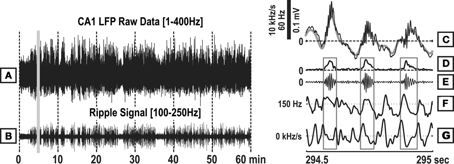
Figure 1. Illustration of signal processing. (A) LFP recording from stratum oriens of the dorsal CA1 region, sampled at 800 Hz. (B) Bandpass filtered LFP signal between (100–250 Hz) results in typical “ripple” signal. (C) Snapshot of raw LFP data taken from (A) (grey vertical bar), with isolated sharp wave activity in the background (1–25 Hz), (D) ripple signal amplitude envelope, (E) ripple band signal (100–250 Hz), (F) the instantaneous frequency (iFreq) estimate, and (G) the frequency modulation (FM) estimate.
Ripples were detected in the four subjects using an amplitude threshold based method (see Section “Materials and Methods”). The observation intervals for Rat 1, Rat 2, Rat 3, and Mouse were 41, 45, 69, and 65 min, respectively. The respective number of detected ripple events was 931, 1210, 1189, and 1850. The range of ripple event rates was approximately 0.3–0.5 Hz.
Dynamic Frequency Structure of Ripple Events
We began our investigation of ripple frequency structure by examining the statistics of peak-aligned ripple events (Figure 2
). We first noted that the median waveform of the amplitude envelope, MUA, iFreq, and FM traces were qualitatively and quantitatively consistent across the three rat subjects and one mouse subject. This was supported by the observation that the 50% confidence interval of any subject contained the median waveform of all three other subjects for any of the four signals. In Figure 2
, this observation is visualized using the empirical 50% confidence intervals of Rat 1.
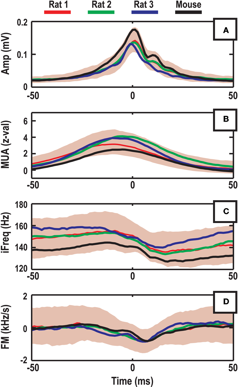
Figure 2. Ripple triggered statistics of (A) amplitude envelope, (B) normalized multi-unit activity, (C) iFreq measure, and (D) FM measure. The red, green, and blue lines are median waveforms of data from three different rat subjects, while the solid black line represents one mouse subject. The solid patch in the background represents the empirical 50% confidence bound computed with the Rat 1 data set.
The median amplitude envelope is a smooth unimodal curve with a baseline of ∼0.025 mV and peak amplitudes in the range of ∼0.1 to ∼0.18 mV (Figure 2
A). In Figures 2
B,C, we observe that the MUA and iFreq signals peak coherently and prior to the amplitude peak of the ripple. In a window of ∼3–5 ms before the amplitude peak of the ripple, the frequency of the ripple begins to decrease abruptly and continues to decrease passed the apex of the ripple envelope. This negative frequency modulation can easily be seen in Figure 2
D as the median FM waveform dips below 0 Hz/s at the point of the ripple amplitude peak. A visual comparison of iFreq and FM (Figure 2
C vs. Figure 2
D) reveals a significant reduction in median waveform variation between subjects for the FM signal. This is largely attributed to the effect that differentiation has on removing constant offsets.
The median structure of the ripple waveforms were consistent across subjects, however, we also noted some degree of variability (Figure 2
). In order to investigate this variability, we extracted features from each ripple and explored their distribution (Figure 3
). The max., mean, and min. values of iFreq and FM were found to be significantly different (p < 0.001 for all subjects), highlighting the dynamic nature of intra-ripple frequency and frequency modulation (Figures 3
D,E). The relationship between SPW phase and ripple activation may be of physiological interest as the underlying excitatory drive corresponding to different phases of the sharp-wave may influence the frequency dynamics of ripples. Sharp wave activity was extracted from the raw LFP and differentiated to obtain an amplitude modulation signal (SPW-AM). Since the LFP of these four subjects were recorded in stratum oriens/pyramidal, the onset of the SPW is indicated by positive values of SPW-AM, while the SPW offset is indicated by negative values. The SPW-AM distribution was not significantly biased towards positive or negative values (Figure 3
C). The mean of the SPW-AM distribution was approximately 1.3, −1.0, −2.8, and 1.6 mV/s for subjects Rat 1, Rat 2, Rat 3, and Mouse. In the same order, the median of the SPW-AM distribution was approximately 0.9, 0.2, −2.9, and 1.6 mV/s.
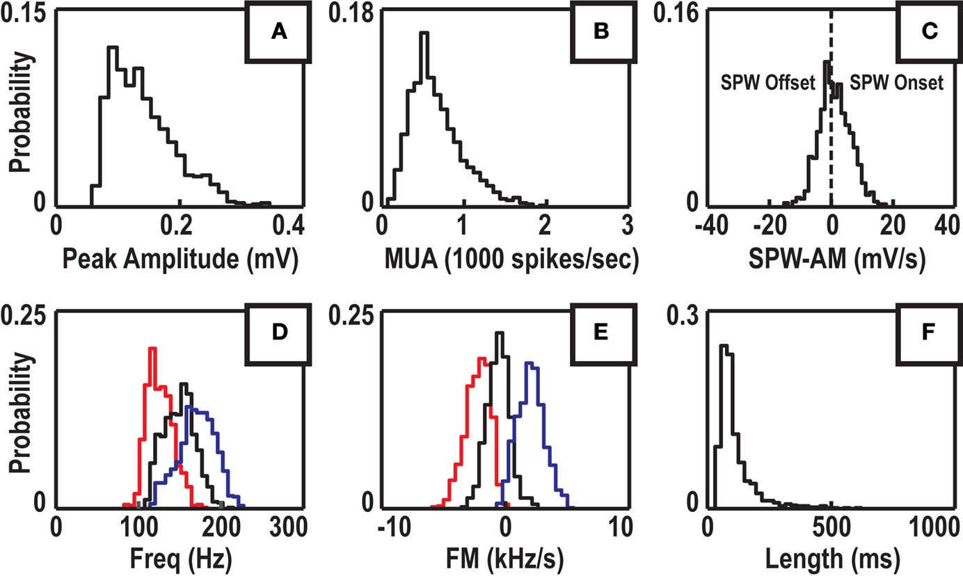
Figure 3. Probability distribution of ripple features for Rat 1. (A) Maximum of the ripple amplitude envelope. (B) Maximum value of multi-unit rate within ripple. (C) Amplitude modulation of sharp wave signal (1–25 Hz) measured around the time of the ripple peak. (D) Max., mean, and min. frequency within ripple. (E) Max., mean, and min. frequency modulation within ripple. (F) Length of ripple. For (D) and (E), the max., mean, and min. curves correspond to the max., mean, and min. values in a 20 ms window about the ripple peak.
Covariation of Ripple Features
Next, we attempted to determine how ripple features were related to one another (Figure 3
). A correlation coefficient (R) was computed for each combination of features (Figure 4
; Table 1
). The majority of correlations were found to be significant, but not necessarily large. The strongest significant correlations were between Amp vs. MUA (R ∼ 0.57, p < 0.001; Figure 4
A) and Freq vs. MUA (R ∼ 0.46, p < 0.001; Figure 4
H). Interestingly, the correlation between Freq and FM was consistently negative across animals (R ∼ −0.18, p < 0.001; Figure 4
I). The Amp vs. SPW-AM, (R ∼ 0.08, p < 0.01; Figure 4
D), and MUA vs. SPW-AM, (R ∼ 0.07, p < 0.01; Figure 4
G), correlation were found to be positive in three out four data sets; the negative correlation for Rat 3 could not be verified as an outlier and, therefore, was used to compute the average correlation.
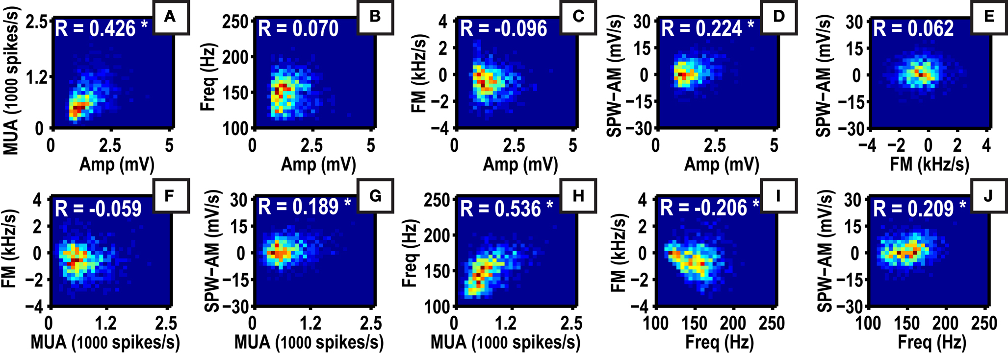
Figure 4. Covariation of ripple features for Rat 1. (A–J) Two dimensional histograms represent the relationship between all combinations of ripple features shown in Figure 3
. These data are taken from Rat 1. The correlation coefficients for each feature combination are shown in white text (the asterisk denotes a correlation with p < 0.001). See Table 1
for a summary of feature correlations for all data sets.
Quantifying Ripple Variability with Frequency Dynamics
The feature distributions in Figure 3
suggest that ripples vary greatly in terms of their amplitude, frequency, and multi-unit properties. We aim to determine if these variations are a systematic property of hippocampal processing or the result of some random noise process. We begin by grouping ripple events based on frequency information (Figure 5
). These two feature dimensions were chosen for their weak but significant correlation and are not directly a function of ripple amplitude (Table 1
). Orthogonal dividing lines for Freq and FM dimensions were used to partition the data. The frequency boundary was chosen to be the median of the frequency distribution (Figure 3
D), which was 150.13 Hz for Rat 1 (146.8, 149.25, and 139.5 Hz for Rat 2, Rat 3, and Mouse). The FM boundary was always chosen to be 0 Hz/s, which allowed for straightforward interpretations of the resulting partitions.
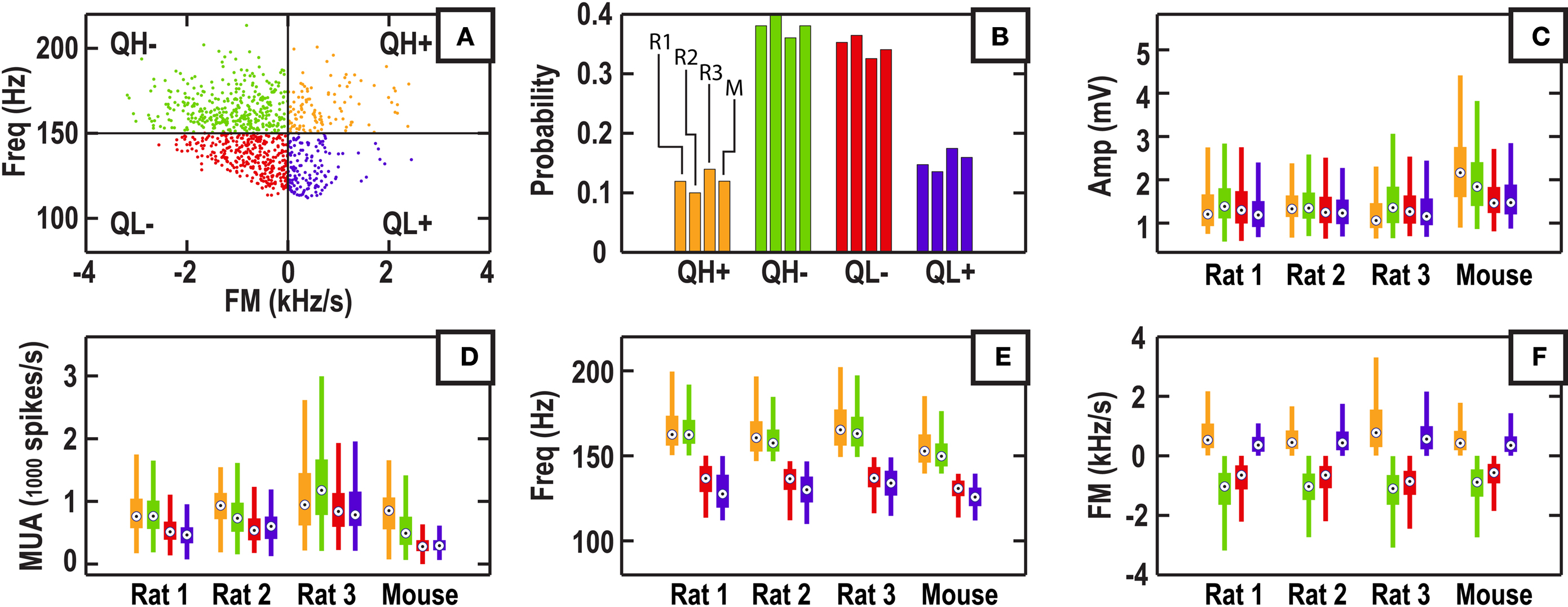
Figure 5. Partitioning of ripple events based on frequency information alone. (A) The boundaries for partitioning are drawn at 150 Hz and 0 kHz/s. QH+ represents high frequency and positive FM, QH− represents high frequency and negative FM, QL− represents low frequency and negative FM, QL+ represents low frequency and positive FM. (B) Relative number of events per partition quadrant for three rat subjects and one mouse subject. (C–F) Standard box-and-whisker plots (95% CI) for features of each partition and each data set. Plots are grouped by subject rather than quadrant.
For Rat 1, out of the 931 ripple events that were originally identified, ∼12% of the events fell into the high frequency, positive FM category (QH+), ∼38% into the high frequency, negative FM category (QH−); ∼35% in the low frequency, negative FM category (QL−); ∼15% into the low frequency, positive FM category (QL+). The relative number of events between the four partitions was markedly consistent across the four subjects (Figure 5
B), demonstrating a consistent bias towards negative FM in the population of ripple events. The average FM was largest in magnitude for the QH− partition across subjects (Figure 5
F), consistent with the negative correlation between iFreq and FM (Table 1
). Feature distributions were compared within subject and between all combinations of partitions (Figures 5
C–F). We found no significant differences in distributions for ripple amplitude between all pairs of partitions (p > 0.05). MUA distributions were significantly different between high and low frequency partitions, but not between positive and negative FM partitions (p > 0.05), consistent with the feature correlations shown in Table 1
. These similarities and differences in partitions properties are consistent across subjects. Representative data examples of ripples from the four partitions are shown in Figure 6
.
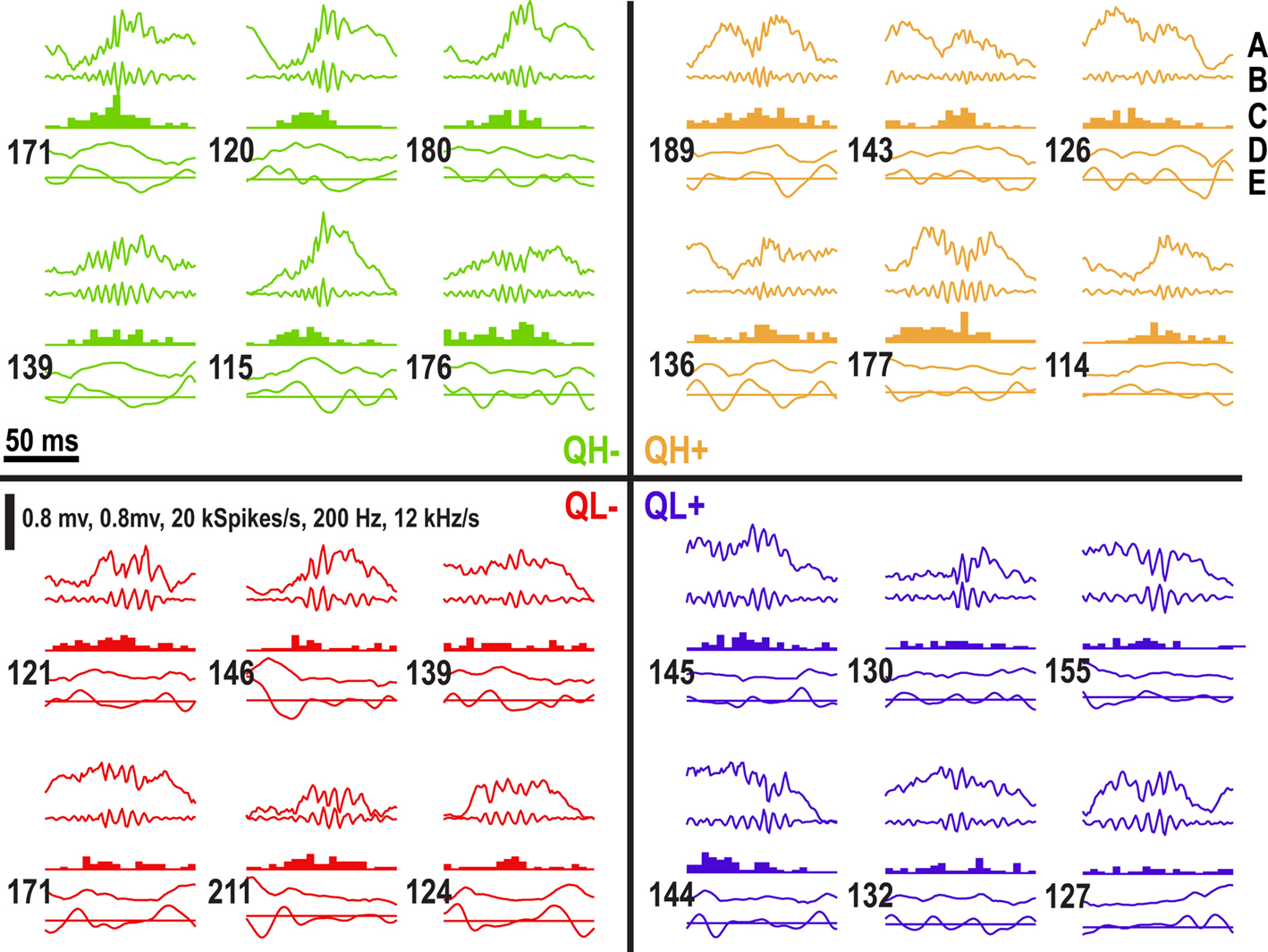
Figure 6. Real data examples from each partition. Each segment is 100 ms long and is centered about the peak of the ripple. (A) The raw data, (B) the ripple signal, (C) the MUA, (D) the iFreq signal, and (E) the FM signal are displayed for each ripple event. The number shown next to the iFreq estimate is the value of iFreq at the beginning of the trace. The horizontal line through the FM signal is the zero line.
In order to better understand how these partitions differ in spectral-temporal dynamics, we computed ripple-triggered averages (aligned by maximum ripple peak) for the ripple amplitude envelope, MUA signal, iFreq signal, and FM over a 200 ms window (Figure 7
). The most striking result is the clear difference in average iFreq and FM structure between partitions. In comparison to the waveform statistics in Figure 2
, these waveform averages demonstrate that average ripple frequency dynamics within quadrants have a larger than expected dynamic range. Moreover, we find in contrast to the no-partitioning statistics in Figure 2
, that ripples can peak in FM before or after the ripple amplitude peak, and that the direction of maximum FM may be either positive or negative (Figures 7
C,D). In addition, the high frequency partitions (QH+ and QH−) are clearly associated with higher MUA, while the low frequency partitions (QL+ and QL−) are associated with lower MUA, which is compatible with the high correlation coefficient between MUA vs. Freq (Table 1
).
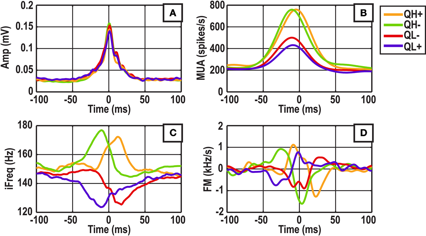
Figure 7. Ripple triggered averages by partition. All feature waveforms are aligned by the time of the ripple center. The panels show average (A) ripple envelope, (B) multi-unit rate, (C) instantaneous frequency, and (D) frequency modulation.
In all partitions, the average FM waveforms indicate that ripple events tend to contain both positive and negative frequency modulation corresponding to increases and decreases of the iFreq (Figure 7
D). In order to quantify this statement, we computed two sets of statistics for all partitions: (1) the percentage of ripple events with either large positive FM or large negative FM peak or both, and (2) the percentage of ripple events containing both large positive and negative FM peaks. For the first statistic, we found the percentage of events that met this criterion to be ∼92.2, ∼95.0, ∼85.2, and ∼79.0% for partitions QH+, QH−, QL−, and QL+, respectively, after averaging the percentages across subjects (Table 2
). In the same manner of computation as the first statistic, the second statistic was found to be 55.0, 60.8, 35.9, and 35.0%, respectively (Table 2
). Therefore, although the average FM waveforms in Figure 7
D indicate some degree of bi-phasic FM modulation, it is more accurate to conclude that individual ripple events in QH+ and QH− robustly exhibit at least one phase of either large FM, while events in QL− and QL+ have a strong tendency to exhibit at least one phase of large FM.
The iFreq dynamics for all partitions appear qualitatively different in Figure 7
C. In order to better quantify the relationship between ripple amplitude dynamics and ripple frequency dynamics within partitions, we first isolated ripple events with large positive and negative FM using the previous analysis. We then assigned each of these ripple events to one of the following categories: (1) both maximum and minimum iFreq occur before, (2) only the min. iFreq occurs before, (3) only the max. iFreq occurs before, or (4) both min. and max. iFreq occur after the amplitude peak of the ripple. We found that the expected frequency dynamics for all partitions in Figure 7
C were consistent with the distribution of events over the four categories (Table 2
, Panels A,B). Our analyses show that for QH−, ∼81% of the considered events belong to category 3 and ∼11% belong to category 1; this can be restated as ∼95% of events have max. iFreq extrema before the ripple peak. For the QL+ partition, ∼62% of events belong to category 2 and ∼23% of events belong to category 1, which together state that ∼85% of events have their min. iFreq extrema before the ripple peak. In consideration of QH+, ∼60% of events belonged to category 2 and ∼16% belonged to category 4; it follows that ∼76% of the events for QH+ have max. iFreq extrema after the ripple peak. For the QL− partition, ∼76% of events belong to category 3 and ∼9% belong to category 4; therefore, ∼85% of events have their min. iFreq extrema after the ripple peak. Although each category contains a non-zero number of events, the consistent ranking of categories within partitions and across subjects suggests that the average frequency dynamics of each partition can be primarily explained by one dominant amplitude-frequency coupling.
Ripple Detection using Frequency Information
A prerequisite problem in the analysis of ripple activity is deciding when a ripple event begins and ends. The most common approach is to compute a signal that is analogous to the instantaneous power in the ripple-band, and set upper and lower amplitude thresholds (AMP detection). The upper threshold is used to locate the approximate location of the ripple while the lower threshold is used to determine the extent of the ripple in time. The threshold based method may be chosen for its simplicity with the understanding that it lacks a robust mechanism for choosing optimal thresholds, and more specifically minimizing Type I (unidentified ripples) and Type II (including noise) errors.
One possible way to improve threshold based ripple detection is to harness the stereotypic frequency profiles of ripples (Figures 2 and 7
). We developed a novel ripple detection algorithm by combining amplitude and frequency information (AMP + FM detection). Figure 8
illustrates how the AMP detection method differs from the AMP + FM detection method. The new detection signal may be viewed as a signal that is highest when there is an increase in ripple band power and an increase in FM within a short temporal window (<10 ms). The rationale for this method is clear from Figure 7
, where large magnitudes of FM and ripple amplitude coincide within a window of 10 ms, on average. The result of ripple detection using only amplitude information is the event set A. The result of AMP + FM detection is the event set AF.
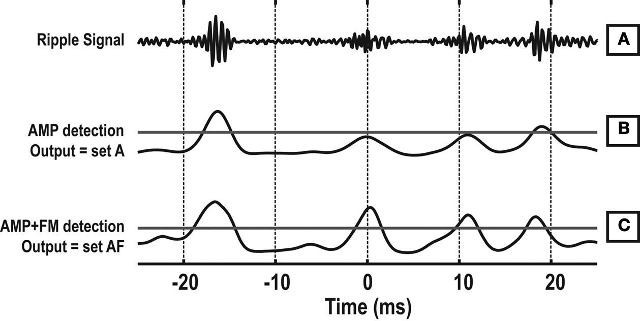
Figure 8. Example of ripple detection using combined frequency and amplitude information. (A) The ripple band signal. (B) The amplitude envelope of the ripple band signal, which is normally used for ripple detection. The horizontal line is the detection threshold. (C) The proposed detection signal that contains amplitude and frequency information. The horizontal line is the detection threshold.
The performance of the AMP vs. AMP + FM based detection algorithms were quantified by, first, identifying the ripple events that were common (A + AF) and those that were mutually exclusive for the two detection methods (A − AF and AF − A; see Figure 9
A). The A + AF set of events were obtained by finding temporally overlapping events in set A and set AF and keeping only the intersection between those events. Next, the events in set A that did not overlap with any events in set A + AF constituted the set A − AF. Likewise, the events in set AF that did not overlap with any events in set A + AF constituted the set AF − A.
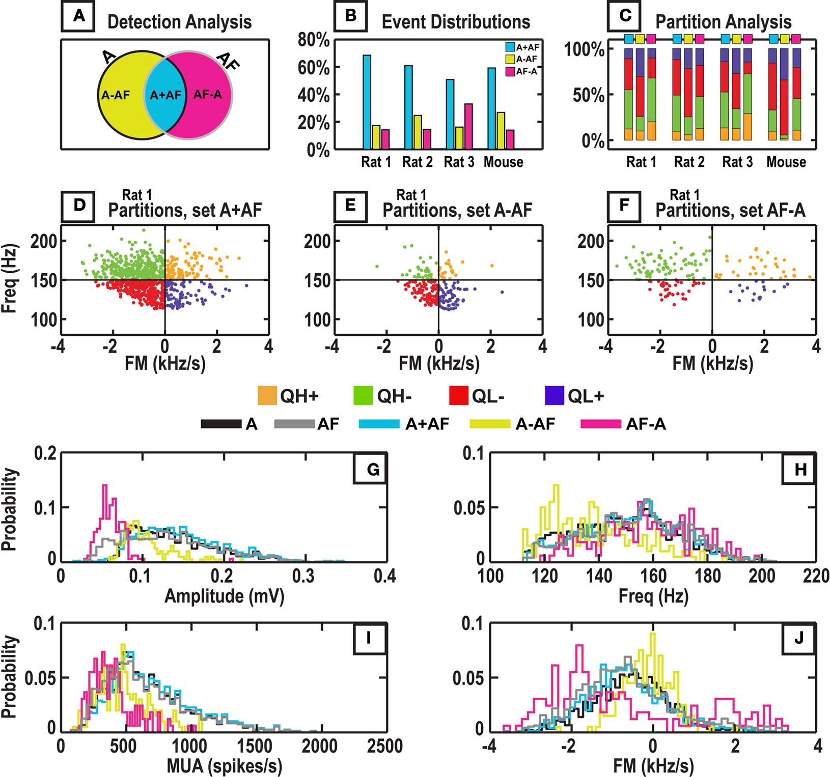
Figure 9. Performance of ripple detection using amplitude information alone “A” and combining amplitude and frequency information “AF”. (A) A Venn diagram showing the evaluation of the ripple detection algorithms. (B) Considering all ripple events proposed, A and AF, this bar graph shows their distribution on the sets of the Venn diagram. (C) For each bar in (B), this graph displays the distribution of events in terms of Freq-FM quadrants. (D,E,F) Each dot represents a proposed ripple event. (G–J) Feature distributions for each set are shown for Rat 1.
Simple set operations dictate that the number of events combined between sets A + AF and A − AF should equal the number in set A; this should also be true when the sets A + AF and AF − A are compared to set AF. However, this equivalence assumes that each ripple event is atomic and cannot be divided further into separate events. In practice, sharp-wave ripple complexes that occur close together in time may be lumped as a single “long” ripple event. When set A and set AF are combined, the intersection of the sets may result in the truncation of “long” ripples into sub-events. Because “long” ripple events in a set may be counted multiple times while merging two sets, the number of events in sets A + AF and A − AF may be greater than that of set A, and the number of events in sets A + AF and AF − A may be greater than that of set AF (Table 3
).
The AMP + FM detection was able to find a large number of candidate events. Across the four subjects, the number of candidate events proposed by the AMP + FM detection ranged from ∼86 to 128% of the number events proposed by the AMP detection method. Of the events proposed by the two methods, the number of events found to overlap (A + AF) was ∼70 to ∼85% of the AMP set, and ∼61 to ∼83% of the AF set (Table 3
).
The A − AF set represents the advantage of AMP detection over AMP + FM detection and vice versa for the AF − A set. Therefore, by examining the characteristics of the A + AF, A − AF, and AF − A sets, we may better interpret the output of the two detection methods. In Figures 9
D–F, we see that the proposed events for the three different conditions span all four pre-defined quadrants for the data from Rat 1. A summary of this partitioning may be found in Figure 9
C, for each of the four subjects; the structure of the stacked bar graph indicates that the A − AF set consisted primarily of events in the QL+ and QL− (low frequency) partitions, while the AF − A set consisted primarily of events in the QH+, QH−, QL− (negative FM or high frequency) partitions. In addition, the largest represented partition in the A − AF set is the QL− partition. The AF − A class consistently contained a larger percentage of QH− events relative to the A + AF set.
Next, we examined the associated feature distributions of event set: A, AF, A + AF, A − AF, and AF − A (Figures 9
G–J). The distribution for ripple amplitude clearly shows that the AF − A set contains only small amplitude events; this is almost certain given that the AMP detection method will have already found all the large ripple amplitude events. The ripple amplitude distribution for A − AF has a lower mean than that of A, AF, and A + AF. The Freq distributions were not significantly different between sets A, AF, A + AF, and AF − A; the Freq distribution was significantly shifted to the left for the A − AF condition (p < 0.001). The FM distributions were significantly different for all set combinations except between the A, AF, and A + AF sets (p < 0.001). Additional insight into the differences in detection sets may be gained by examining events from sets A + AF, A − AF, and AF − A (Figure 10
).
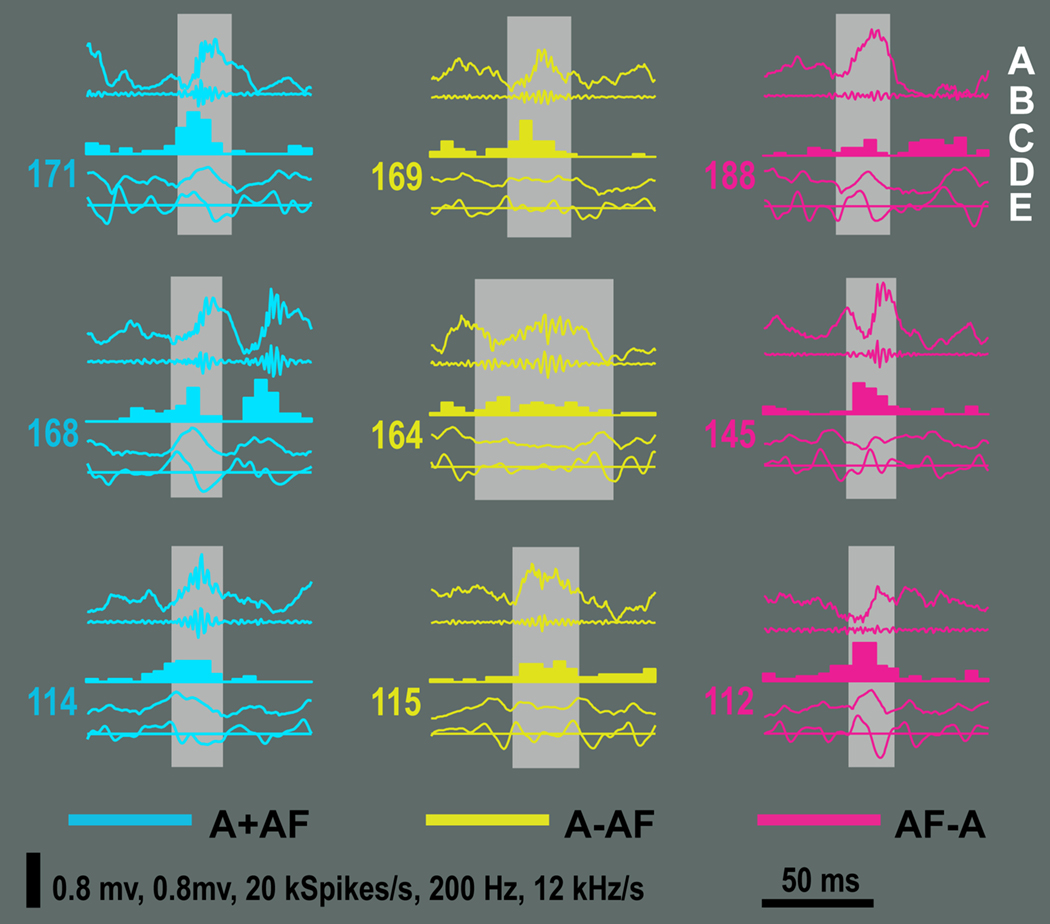
Figure 10. Examples of ripples from the mutually inclusive (A + AF) and mutually exclusive categories (A − AF and AF − A). The order of the traces for each example is (A) Raw LFP, (B) ripple band signal, (C) multi-unit activity, (D) iFreq signal, and (E) FM signal. The horizontal line in (E) marks 0 kHz/s. Each example is 100 ms in duration.
We additionally quantify the characteristics of the AMP vs. AMP + FM detection by computing two measures of activity: (1) MUA, which is a quantity known to be associated with ripple activity but does not depend on the presence of ripples, and (2) gamma-ripple score, which compares high gamma-power (70–100 Hz) to ripple band power (100–250 Hz) to determine if an event may possibly be a high-gamma process. We found across subjects that the average MUA rate was not statistically different between set A and set AF, between set A and set A + AF, and between set AF and set A + AF (p > 0.05). The set A + AF had the largest average MUA rate of all five sets. The sets A − AF and AF − A had lower average MUA rates compared to set A + AF. The average MUA rate for AF − A was either lower than or equal to A − AF (Table 3
). In our analysis of gamma vs. ripple band power, we report the percentage of events where gamma power exceeds ripple power (Table 3
, Panel D). The set with the largest percentage of positive gamma-ripple scoring events is AF − A (∼7.5%, p < 0.005), followed by set AF (∼2.3%, p < 0.001). In general, the sets with the lowest percentage of events with positive gamma-ripple score are sets A (0.74%, p < 0.001), A + AF (0.80%, p < 0.001), and A − AF (0.68%, p < 0.001). We systematically altered the bandwidth of the gamma-band and found that the percentage of gamma-dominated events increased for all event sets across all subjects as the bandwidth was increased, and decreased for all event sets as the bandwidth was decreased. While the percentages here reflect the specific case where the gamma-band is 70–100 Hz, the assertion that set AF − A contains the largest proportion of gamma-dominated events is generally true for different gamma bandwidths across all subjects.
The fine temporal-spectral analysis of ripple frequency dynamics provides a foundation for exploring the neurobiological significance of hippocampal ripple activity. We demonstrate this by showing that ripples have consistent variation in frequency structure across multiple rat subjects, and in both rat and mouse species. In addition, we show that frequency modulation (FM) is a measurable quantity that can be used to selectively group ripple events with similar frequency characteristics. In order to address the problem of ripple detection, we devised a novel ripple detection procedure that incorporated the known amplitude signature and the here established FM signatures of ripples.
Ripple Frequency Dynamics
We investigated the variation in ripple frequency structure by examining sub-populations of ripple events based on Freq and FM features. We chose orthogonal boundaries in the Freq and FM dimensions heuristically: the median of the Freq distribution was the Freq boundary, and 0 kHz/s was the FM boundary. We choose these heuristics for straightforward interpretation of the results. We partitioned the Freq-FM plane into four quadrants: QH+, QH−, QL−, and QL+ (Figure 5
A). We were careful to refer to the sub-populations as quadrants or partitions and not “classes”, as the word “class” may imply the representation of a distinct physiological process. The number of ripples assigned to each partition was consistent across three rats subjects and one mouse subject (Figure 5
). One criticism of this consistent pattern across data sets is the heuristic we use by definition divides the population in half in the Freq dimension (median). However, the boundary in the FM dimension is always fixed at 0 Hz/s, and, therefore, is not adjusted by the distribution of the FM feature. The consistent distribution of features across subjects suggests that the variation in amplitude-frequency dynamics is natural property of neural processing in the rodent hippocampus.
The quadrant with the greatest number of events (QH−) contained events with a strong tendency to increase in frequency before the amplitude peak and abruptly decrease in frequency during the peak (Figure 7
); this quadrant also retained large correlation coefficients between MUA vs. Freq and MUA vs. Amp. The next populous quadrant was QL−, which contained events that kept a constant frequency at the onset of the ripple and dropped in frequency during the peak of the ripple. These two partitions representing negative FM made up ∼75% of all observed ripples. A smaller and significant percentage (∼25%) of ripple events belonged to the QH+ and QL+ partitions. These events tended to increase their frequency abruptly after the amplitude peak of the ripple (QH+), or tended to decrease their frequency abruptly before the peak of the ripple and then rebound in frequency during the ripple peak (QL+), leading to a positive FM during the peak of the ripple (Figure 7
).
Although Figure 2
suggests a single stereotypic frequency structure within ripples, we later found that the strong tendency for negative FM only applied to a subset of ripples (Figure 5
). The variable relationship between ripple amplitude, frequency, and FM was visualized in Figure 7
. These temporal differences in amplitude and frequency dynamics are also reflected in their correlations (Table 1
); while the correlation between Freq vs. MUA and Amp vs. MUA was high, paradoxically, the correlation between Freq vs. Amp was low (Table 1
). These correlations suggest that the amount of MUA activity can explain ∼20–30% of the variation in both Amp and Freq, while Amp and Freq may only explain less than 1% of each other’s variation. Figure 2
displays a tendency for the temporal peak of the MUA to coincide with the temporal peak of frequency, which suggests that the peak in ripple frequency represents an apex in neural coordination. However, Figures 7
C,D show that when ripple events are grouped by similar frequency and FM properties, the expected peak of frequency dynamics need not coincide with that of MUA. Therefore, we focused on quantifying the number of positive and negative FM extrema for each ripple event. Based on our analyses (Table 2
, Panels A,B), we concluded that generally four out of five ripples have at least one large extrema, one-half of the ripples in the high frequency partitions (QH+ and QH−) had two large extrema, while one-third of the ripples in the low frequency partitions (QL+ and QL−) had two large extrema. In addition, we then categorized ripple events based on their amplitude and iFreq dynamics (Table 2
, Panel C) and found that ripples were dispersed throughout the categories, however, different partitions had different biases for categories; these biases consistently explained the average iFreq waveforms seen in Figure 7
C. Thus, while MUA and ripple amplitude are highly correlated (Table 1
) and maintain a consistent temporal relationship (Figures 7
A,B), the small timescale correspondence between population activity and iFreq is not as straightforward (Figure 7
). Embedded in the MUA population measure are coordinated spiking activities that are likely variable over time and space for each individual ripple event.
These variations in amplitude-frequency dynamics may be explained by the phasic, repetitive participation of specific interneuron types and pyramidal cells during the start, middle, and end of the ripple. For example, oriens lacunosum-moleculare (O-LM) and axo-axonic cells are most active at the early stage of each ripple event while pyramidal cells are most active at the center of the ripple event (Behrens et al., 2005
; Klausberger et al., 2003
; Maier et al., 2003
; Spampanato and Mody, 2007
). Frequency modulation during the ripple peak is most likely determined by synchronous spike frequency adaptation of individual units in response to both intrinsic receptor dynamics and network properties (Dzhala and Staley, 2004
; Foffani et al., 2007
; Gollisch and Herz, 2004
). A characteristic of pyramidal cell bursting is that with each successive spike the inter-spike interval is more variable than the first and towards the end of the burst the desynchronization of population activity emerges. Hence, the tail of the ripple may likely represent a decrease in synchrony between pyramidal cells and an increase in activity of axo-axonic, O-LM, and radiatum lacunosum-moleculare (R-LM) interneurons (Dzhala and Staley, 2004
; Klausberger et al., 2003
; Spampanato and Mody, 2007
). The variability in amplitude-frequency dynamics of ripples, therefore, may partly be accounted for by neuromodulatory factors that lead to changes in excitation/inhibition of specific interneuron types and pyramidal neurons.
In the interpretation of our results, we considered how the frequency dynamics of ripples may change as a function of space. We first reasoned that relatively low amplitude ripple events may either be due to limited participation of neuronal populations or represent a high amplitude event that is generated at a distance from the recording electrode. Next we considered the MUA trace to be a more global measure of neuronal activity that is less sensitive to spatial distortion since MUA is derived from pooling local action potentials over several electrodes. If changes in frequency dynamics were caused by volume conduction, then we would expect to find a high correlation between ripple amplitude and frequency characteristics, while finding a low correlation between MUA and frequency characteristics. On the contrary, we found in Table 1
that the correlation coefficient between amplitude vs. frequency, and amplitude vs. FM was small. In addition, the correlation between MUA vs. frequency was high. Furthermore, we found a marked difference in MUA distributions between high frequency and low frequency partitions (Figure 5
D). This evidence suggests that the variation in frequency-FM were not primarily caused by spatial distortion of volume conducted oscillations; instead, this variation is more likely a function of how many neurons are active during a ripple event and the small timescale interactions of neurons that underlie ripple activity.
Ripple Detection using Frequency Dynamics
The problem of ripple detection may be viewed as a classification problem, where the goal is to classify the signal (ripples) from the background noise. A challenge is to first establish a concrete definition of the “signal” so it may be properly detected. Here, we do not propose to solve this problem of defining a ripple. Instead, we suggest that frequency modulation profiles observed in Figure 7
may be harnessed to improve the process of ripple detection. First, we noted that regardless of the quadrant of the ripple, the greatest magnitude of FM occurred in a ±5 ms window of the ripple peak (Figure 7
D). By rectifying the FM signal and smoothing it, we were able to create a FM information signal. Using this signal alone resulted in a large number of false positives. In order to address this, we combined amplitude and FM information by multiplying the ripple envelope signal with the FM information signal (Figure 8
). The result was a signal that was large when there was a combination of the large amplitude and/or large FM. We referred to this method as the AMP + FM method for ripple detection.
We compared the AMP + FM method against the commonly used amplitude-based method (AMP). In order to quantify the performance of the AMP + FM method, our goal was to understand what events the AMP + FM method could and could not identify relative to the AMP method. The Venn diagram in Figure 9
A shows a schematic of the analysis we performed. After performing ripple detection with both methods, we performed a detailed investigation of the sets A + AF (events common to both AMP and AMP + FM), A − AF (events unique to AMP detection), and AF − A (events unique to AMP + FM detection).
The results of the ripple detection were generally consistent across subjects. The number of ripple events proposed by the AMP + FM method was similar to that proposed by the AMP method on average (Figure 9
B; Table 3
). We examined the MUA distribution for each event set (Table 3
). In comparison, the set with the largest mean MUA was the mutually inclusive set A + AF; the sets with the next largest average MUA were sets AF and A, with set AF having a slightly larger average MUA. The set A − AF had the second to lowest average MUA, while AF − A had the lowest. In analyses that compared RMS gamma power vs. RMS ripple power, we found that the event set AF − A had the greatest percentage of gamma-dominated events (∼7.5%, p < 0.005, gamma band = 70–100 Hz), while other event sets contained much smaller percentages (less than 2.5%, Table 3
). Visual inspection of gamma-dominated events in set AF − A revealed noticeable concentrations of power between 80 and 120 Hz. As these events straddle the 100 Hz dividing boundary between ripple and gamma events, it is not possible to determine by using our analyses if these events are distinct within themselves or represent the continuum of either the gamma or ripple process. However, if we consider gamma-dominated events to be events that are not ripple events, the set AF − A contains the largest percentage of false-positives at approximately 7.5%.
We also examined how the components of the sets A + AF, A − AF, and AF − A were divided into quadrants: QH+, QH−, QL−, and QL+. We consistently found that the majority of the AF − A set belonged to the QH− class, which we established before as the partition that normally contains the greatest number of ripple events, as well as the partition with the largest correlation between Freq vs. MUA. Moreover, the distribution of ripple events in the Freq-FM plane for set AF − A was consistently more similar to that of set A + AF (Figure 9
); the same statement cannot be generalized when comparing set A − AF to set A + AF.
The AMP + FM method finds an additional 17% more events compared to the AMP method. These additional oscillatory events were lower in amplitude and MUA compared to events found by the AMP method of detection. Approximately 7.5% of these additional events were found to be more gamma-dominated (gamma power > ripple power). Assuming these gamma-dominated events are false-positives, we conclude that the AMP + FM method, when combined with the AMP method, locates 15% more ripple events than the AMP method alone.
The AMP and AMP + FM based detection methods may be combined in different ways to address Type I (false positive) and Type II (false negative) errors. We note that the set A + AF is a set with the largest average MUA and is well-distributed in ripple amplitude, frequency, and FM. In this case, retaining the events set A + AF may help to minimize the possibility of false positives. Alternatively, the AMP + FM based detection may be used to address Type II errors (false negatives) as well; events in the AF − A set may represent physiologically meaningful events that fall below the detection threshold of the AMP based method, and, therefore, would incorrectly be classified as noise. Based on our conclusions of the gamma-band analysis above, approximately 92.5% of the events in AF − A are expected to contribute to the reduction of Type II errors.
The results presented here may facilitate future work in the decoding of hippocampal network activity in a neurobiological context. With more precision in ripple characterization, we gain additional ability to distinguish between distinct neural processes. Ripple features that are highly correlated help to constrain our thinking and infer possible causal mechanisms. These principles may be applied in vitro to build a vocabulary for interpreting ripple activity in vivo, as in Ponomarenko et al. (2004)
. Such analytical capabilities may prove useful in determining the neural substrates of memory related phenomena such as forward or reverse replay (Diba and Buzsaki, 2007
; Foster and Wilson, 2006
).
These variations in ripple amplitude and frequency dynamics may be further examined by treating the dynamic frequency trace like an action potential waveform, and utilize spike classification techniques such as Bayesian mixture model analysis in combination with dimension reduction techniques to cluster the ripple events (Lewicki, 1998
; Nguyen et al., 2003
; Shoham et al., 2003
). Such approaches may provide the ability to precisely target analyses to physiologically specific events.
In conclusion, the advancements made here directly address current challenges in the study of ripple activity with respect to hippocampal function. We demonstrated that the dynamic frequency structure of ripple events may be quantified with high spectral and temporal resolution. We observed variations in amplitude-frequency dynamics of ripple oscillations, which were markedly consistent between multiple rat subjects and one mouse subject. We exploited the dynamic frequency information to explore the variation of ripple events. We found that the majority of proposed ripple events had a strong tendency to be negatively frequency modulated, however, a significant population were positively modulated. In addition, we found that the relationships between ripple amplitude and frequency dynamics were not intimately constrained to one template. Finally, we showed that the frequency structure of ripples may be used to detect ripples that would not be found otherwise, as well as reduce the Type I and Type II errors.
We have no conflicts of interest to disclose.
This work was funded in part by the following grants: NIH/NIMH R01 MH59733, NIH/NIHLB R01 HL084502, and the Singleton Graduate Student Fellowship. We thank members of the Wilson Lab, Brown Lab, and Tonegawa Lab for helpful comments.