Adaptive transition rates in excitable membranes

Introduction

Cellular excitability is a fundamental physiological process (Hille, 1992) whereby voltage-dependent changes in membrane ionic conductance lead to an action potential, a threshold-governed transient in cross-membrane voltage, v. Hodgkin and Huxley (1952) formalized a generic biophysical mechanism underlying the generation and propagation of action potentials. In this formalism, as well as in its later extensions, the flow of ions down their electrochemical gradients is modulated by the probability of ionic “channel” proteins to reside in the so-called open (i.e. conductive) state. Non-linearity arises from the voltage-dependent reaction rates governing the transitions of channels between the conductive and the non-conductive states. For membrane excitability under physiological conditions, at least two populations of channel proteins are required, one that acts as an exciting force (sodium or calcium conductances) and the other as a restoring force (mostly potassium conductance). The analyses presented here are generally applicable to both types of conductances.

Two kinds of non-conductive states were proposed by Hodgkin and Huxley in their original work: closed and inactive. A generic three-state kinetic scheme (Hille, 1992) is shown below; transition rates pushing to the right are proportional to e^v, whereas left-directed transition rates are proportional to e^−v:

α and β are millisecond time scale voltage-dependent reactions, and are often one order of magnitude faster compared to k_f and k_b. The transition rates between the open and inactive states are in most cases state-dependent rather than strongly voltage dependent, unlike the original Hodgkin-Huxley intuition (see Chapters 18–19 in Hille, 1992, especially p. 622); this difference turns out to be critical for the capacity of channel populations to accumulate inactivation by integrating short-term activities (Manevitz and Marom, 2002; Marom, 1994, 1998; Marom and Abbott, 1994; Marom and Levitan, 1994; Turrigiano et al., 1996).

Fifty years of extensive research into the kinetics of ionic channels show that both the closed and the inactive states of the above three-states scheme are actually sets of many states in any specific channel studied. The set of closed states is rather compact and is functionally proximal to the open state; it is compact in the sense that the involved states are strongly coupled by rapid voltage dependent transitions with a characteristic time scale at the range of milliseconds. In contrast, the set of inactive states is extended; it is composed of a large number of states that are coupled by weak voltage-dependent and voltage-independent transition rates with time scales ranging from milliseconds to many minutes. The emerging picture is summarized in the kinetic scheme below (e.g. Ellerkmann et al., 2001; Hille, 1992; Liebovitch et al., 1987; Marom, 1998; Millhauser et al., 1988a,b; Uebachs et al., 2006):

Here, the set of closed states is represented by a single entity, reflecting the fact that transitions amongst them relax within milliseconds. The wide range of inactivation time scales (beyond six orders of magnitude) makes the choice of how to represent the space of inactive states a more subtle issue. In Eq. 2 the space of inactive states is represented by a one-dimensional cascade of m transitions, without loss of generality (Millhauser et al., 1988a); note, however, that various forms of branching kinetics, with hierarchical transition rates, are fully compatible with the arguments presented in this study.

It is quite clear that the apparent length (m) and internal structure of the inactivation cascade is largely constrained by the resolution and stability of physiological measurements; with the advancement of experimental techniques, more timescales are exposed, leading to interpretations that are expressed in terms of an ever-increasing number of coupled molecular states. Concordantly, present mathematical models of excitable cells may include dozens of coupled differential equations, each of which takes care of a limited range of state transitions. While serving as an inexhaustible source for high-resolution physiological experiments and computer simulations (e.g. Kleber and Rudy, 2004; Markram, 2006), the explanatory value and the mathematical aesthetics of the resulting high-dimensional models are open to question.

Here, an alternative framework is presented; an abstracted population approach to the problem of ionic channel modeling. The approach is realistic in the sense of dealing with the richness of molecular time scales, yet it does not involve concrete accounting for each of an ever-increasing number of molecular degrees of freedom. The model is applied to address the impact of channel population distribution in the space of the inactive states on the dynamics of excitability in general, and activity-dependence over a wide range of time scales in particular.

Results and Discussion

Model

The following analyses rely on a conjecture presented by Millhauser et al. (1988a,b), supported by recent experimental observations (Ellerkmann et al., 2001; Jones, 2006; Melamed-Frank and Marom, 1999; Toib et al., 1998; Uebachs et al., 2006) and computer simulations (Drew and Abbott, 2006; Gilboa et al., 2005; Lowen et al., 1999). The basic idea behind the conjecture is that the immensity of the molecular degrees of freedom underlying cellular excitability allows for a continuum approximation of the relations between activity and the effective rate that governs the dynamics. Somewhat related ideas are exercised in the interpretation of physiological data obtained at different levels of organization and various excitable systems (Fairhall et al., 2001; French and Torkkeli, 2008; Lowen et al., 1997; Lundstrom et al., 2008; Soen and Braun, 2000; Teich, 1989).

Millhauser, Salpeter and Oswald conjectured that, microscopically, the effective rate of transition (denoted δ), from the chain of inactive, unavailable states (I₁, I₂,…,I_m), to the cluster of available (Closed and Open) states, depends upon the depth of the inactive state that the channel occupies (Millhauser et al., 1988a,b). When the dynamics beyond the time scale of the single action potential is considered, the above chain-like kinetics (Eq. 2) are represented by the following abstraction:

in which the set of available states (denoted by A) includes, besides the open state itself, all the states from which the channel may arrive to the open state within the time scale of a single action potential: the closed states and the very first inactive states that are treated in the original Hodgkin and Huxley formalism for the action potential generation. In other words, a channel in A is available for conducting ions within the time scale of a single action potential. The right-hand term of Eq. 3 represents the pool of states from which transition to the open state within the time frame of an action potential is impossible.

Macroscopically, it is instructive to think of A in the context of G_max, the maximal conductance (or number of ionic channels) in a unit area of membrane; in the original Hodgkin and Huxley formalism, G_max is a structural constant that sets limits on the instantaneous (at the scale of milliseconds) input–output relations of the membrane. But when long-term effects are sought, the effective G_max might be treated as a dynamic variable, modulated by (I₁, I₂,…,I_m), a reservoir that pulls channels away from the system as a function of activity. Such defined, Eq. 3 describes a standard Hodgkin-Huxley “gate” variable (e.g. the “h” inactivation gate). But this is where the Millhauser’s et al. conjecture makes a difference: let Z denote the depth of the inactive state that the channel occupies, such that 1 ≤ Z ≤ m; the larger the Z, the slower the δ, reflecting the multiplicity of transitions along the path I_Z → I₁. Millhauser et al. (1988a,b) showed that in the above scheme, multiplicity of inactive states entails a power-law scaling of δ with Z. Macroscopically, where a strongly coupled single type population of channels are considered, the value of δ is determined by the structure of O(Z), the distribution of channel molecules within the space of non-available states (Figure 1); this distribution defines the long-term (at the range of tens of milliseconds to minutes) input–output relations of the system. Thus, in contrast with standard Hodgkin-Huxley gates, δ does not have a uniquely defined characteristic time scale. Rather, its time scale is determined by the distribution of channels in the space of inactive states, which, in turn, is dictated by the history of activation.

FIGURE 1

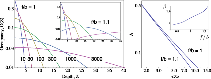
Figure 1. Distributions of occupancy within the inactive cascade ; computed for m = 50 using the generator matrix Q, where P(t) = P(0) exp(Qt), and P(t) is a vector of occupation probabilities. A reflecting barrier was set such that channels are forced to diffuse into the inactive states cascade (i.e. the probability of I₁ → A is set to zero). The depth of any given inactive state in the cascade is depicted on the X-axes (Z). The probability of channels to occupy each Z state depth is depicted on the Y-axis. Different distributions (colored) were induced by setting the reflecting barrier for different time durations (10, 30, 100, 300, 1000, 3000 time units), from an initial condition where the probability of occupying the A state is 1. All transition rates pushing to the right (i.e. forward, depicted “f”) were set to 0.1. The forward-to-backward (f/b) ratio of rates is set to unity in the main panel, and to 1.1 in the inset panel, demonstrating the sensitivity of the family of distributions to transition rates within the cascade. Right: A Log–Log plot of occupancy of A, the available set of states, as a function of the first moment 〈Z〉 of the distribution of channels within the space of inactive states, for the two settings shown in the left panel; (see text). Inset of right panel shows the dependence of β on f/b ratio, calculated by a fit to Eq. 5.

Well-controlled experimental analyses using various kinds of homogeneous populations of ionic channels show that the above prediction of a power-law relation between Z and δ is valid under voltage-clamp conditions (Ellerkmann et al., 2001; Melamed-Frank and Marom, 1999; Toib et al., 1998; Uebachs et al., 2006). In these experiments, the channels are driven into the inactive chain by long lasting activation pulses; a power-law relation, , was found between the duration of the activation pulse, T, and the effective recovery rate δ. During activation (i.e. reflecting a boundary condition enforced by increased membrane voltages due to stimulation), Equation 2 entails a diffusion-like behavior of 〈Z〉 (Millhauser et al., 1988a), the first moment of O(Z), such that (Gilboa et al., 2005). We may therefore write:

with D being a non-negative number, interpreted as the dimension of the unavailable set of states and reflects the constraints on the accessibility to these states (Bassingthwaighte et al., 1994; Liebovitch et al., 1987). The factor, , is an offset that may be thought of as the recovery rate (δ) at Z = 1 or D = 0; for any D > 0, .

As demonstrated both experimentally (e.g. Ellerkmann et al., 2001; Toib et al., 1998; Uebachs et al., 2006) and numerically (e.g. Gilboa et al., 2005; Marom and Abbott, 1994), the state-dependency of inactivation (Eq. 1) fosters accumulation of slow inactivation by spike series or spike-like voltage pulse series, and entails scaling of recovery rates (Eq. 4).

Crucial for what follows is to note that while δ is determined by the statistics of a seemingly “hidden” distribution of a population of channels in the space of inactive states, unique and direct information about the value of 〈Z〉 is given in the fraction of channels that remains in the cluster of available (A) states (Gilboa et al., 2005; Millhauser et al., 1988a,b). This point is demonstrated in Figure 1; the relation of A to 〈Z〉 is:

where r = 1 may be safely assumed (accounting for maximal availability when Z = 1).

Let us further reduce Eq. 3, by normalizing the total number of channels in the system such that , where P(x) denotes the fraction of channels residing in state x, and obtain:

Thus, the righthand term of Eq. 6, (1 − A), includes all the inactive states from which the open state is not accessible within the time scale of a single action potential; these are the unavailable states. Note that Eq. 6 directly translates to:

In what follows, γ, the rate of loss into the non-available set of states, is assumed to be determined by the frequency of above-threshold activations, which, in many excitable tissues, is quite narrowly distributed notwithstanding fluctuations induced by external input. Thus, in our model γ is a measure of the activity or some monotonic function of it. A further assumption is made, that the compactness of the cluster of available states entails that the exact state within A in which the channel resides does not significantly influence its characteristic time scale for the transition , when long-term effects are considered. Moreover, in the present analysis the amplitude of activation (internally or externally-driven) is assumed sufficient to induce an transition, which is insensitive to whether or not an action potential was evoked; the latter is a very reasonable assumption given known relations between threshold potential and activation of exciting conductances in a wide range of physiological preparations.

The above set of physiologically plausible simplifying assumptions regarding γ proves useful below. But in some sense, γ embodies the environment within which the simple system, resides; hence, more complicated functions can be introduced, aimed at relating γ to the statistics of stimulation frequency and amplitude, the probabilities of obtaining action potentials at a given stimulation regimen, and various history-dependencies (see, for instance, discussion on discrete equation, below).

As shown above (Eq. 4), δ scales with the history of inputs to the cell, thus making the very nature of the system described in Eq. 6 sensitive to its own history of inputs. The impact becomes immediately apparent by rearranging Eq. 5, substituting Z in Eq. 4, and reducing Eq. 7 to:

in which, under constant γ, the dynamics depend on one number, D, a measurable dimension of the inactive state space. Dividing by , letting , , and noting that lead to a reduced, dimensionless form of Eq. 8:

In simplified channel models that are reduced from the classical Hodgkin and Huxley formalism, D → 0, but measurements in realistic channel proteins (Ellerkmann et al., 2001; Melamed-Frank and Marom, 1999; Toib et al., 1998; Uebachs et al., 2006) yielded D estimates ranging from 0.08 to 0.8, an order of magnitude apart, that has far reaching physiological implications, as shown below.

Implications

Dynamic Input–Output relations

Equation 8 implies a change of A, the fraction of channels that reside in the set of available-for-activation states, as a function of input statistics. The environment (electrical or chemical activations) is embodied in γ, whereas the system (ionic channels) is embodied in the form of a single variable, that is D. As shown below, analysis of Eq. 8 leads to insightful conclusions about the nature of excitable membrane responses beyond the time scale of a single action potential in general, and response adaptation of neural activity in particular. But before such an analysis is presented, it is useful to say something more concrete about the meaning of A in general. At some point above, an analogy of A to an effective Hodgkin-Huxley G_max was offered; we are now in a position to further elaborate on this analogy: When A → 1, the effective G_max approaches the standard Hodgkin-Huxley G_max, that is the maximal conductance that is physically available to the membrane when all membrane-residing channel proteins that are selective to the ion on question are open and conductive. Any other value of A (0 ≤ A ≤ 1, by definition), entails an effectively reduced G_max; in other words, the maximal conductance available for a membrane when A < 1 is less than the maximum that is dictated by the physical number of channel proteins residing in that membrane. To the extent that G_max determines the input–output relation of a given Hodgkin-Huxley realization, different values of A entail different input–output relations; hence, dynamics of A is dynamics in a space of possible input–output relations, a space of different Hodgkin-Huxley realizations. Such dynamics may, of course, be introduced by adding more and more Hodgkin-Huxley-like gates, each with a different uniquely defined time scale. Our aim here is to avoid such an approach and let these time scales and entailed dynamics be the result of a mathematically analyzable model rather than its determinants.

Population approach to the dynamics of excitability

In what follows, a population approach is adopted in order to study the impacts of D, the dimension of the unavailable space of channel states, on the dynamics of excitability. Analysis of the continuous model (Eq. 8) is presented, followed by biophysical arguments that justify analysis of a discrete form of the model (Eq. 10). Both analyses indicate that D serves as a “buffer” that contributes to the stability of the system: The continuous model shows that as D increases, the system is less sensitive to high frequency fluctuations around its steady-state solution; the discrete form of the model shows that as D increases, the system becomes less susceptible to bifurcating response modes when activity rates are increased.

Equation 8 has the general form of a Logistic equation. In retrospect, a relation to a Logistic equation should not come as a surprise, for what we are dealing with here is a constrained population of channel proteins, with availability for further activation that is dominated by its own activation history. It is immediately clear that Eq. 8 has one stable solution A*, which is affected by both γ and D. The time scale of the system’s response to a disturbance around the equilibrium is determined by the first derivative of the equation at A*: it increases with D (the dimension of the space of inactive states), as if the latter contributes to the stability of the system by “buffering” fast fluctuations in rates of activity around A* (Figure 2).

FIGURE 2

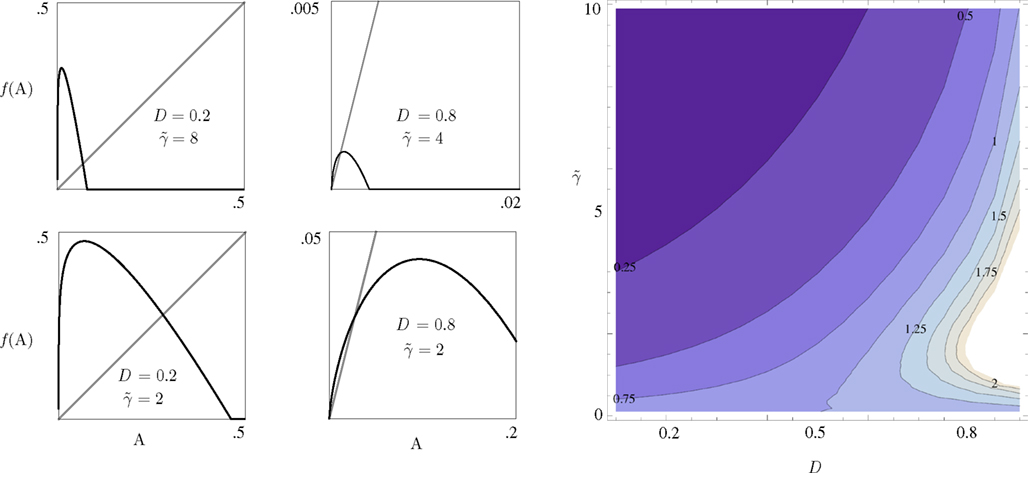
Figure 2. The four panels on the left demonstrate the effect of D and on the dynamics of Eq. 9, where Straight diagonals are depicted for convenient identification of the steady-state solution, A*, where f(A) = A. The contour plot on the right shows the time constant of population response to perturbations around equilibrium, as a function of D and . Color scaling: values of time constant are depicted on contour lines.

The mathematics involved in logistic equations and networks of coupled equations is well developed; its implementations give reasons to believe that phrasing Eq. 8, which results from a molecular level picture, in discrete (map) terms, might prove useful in analyses of single excitable cells and their networks. However, one must be very attentive to the justification of such a path from continuous to discrete form, because of the qualitative nature of its impact on the entailed dynamics. In population models, mapping is used when there is no overlap between successive generations and so the growth occurs in discrete steps (Murray, 1993). As shown below, while a mathematically rigorous path from the continuous form of Eq. 8 to a discrete form is not immediately available, there are good biophysical reasons, supported by experimental results, to think in discrete terms in the context of an excitable cell, where transitions between epochs that are characterized by different degrees of activity are abundant.

To phrase the model in a discrete form, we start by considering a long time series of action potentials, composed of various regions that may differ from each other in the intensity of activity – e.g., firing rate (see Figure 3). Note that such time series are ubiquitous in excitable cells, where bursts of activity at various length superpose ongoing low-level activity. We divide the time series into epochs of activity; T_n, the duration of epoch n, might be different from, or equal to T_{n + 1} (Figure 3). During the n-th epoch, within which activity is expressed in terms of action potentials, the rate of loss into the set of unavailable states, denoted Γ_n, is a function of the intensity of activity (e.g., firing rate) along the n-th epoch (see, for instance, Figure 1C in Toib et al., 1998, or Figure 5 in Ellerkmann et al., 2001). What we learn from experimental voltage-clamp data (e.g. Ellerkmann et al., 2001; Jones, 2006; Melamed-Frank and Marom, 1999; Toib et al., 1998; Uebachs et al., 2006) allows for two assumptions to be made at this stage: (i) The time scale of entry into the unavailable set of states is in the order of many seconds, even tens of seconds. This experimental finding allows us to safely consider a condition in which , while still be within the range of interest, that is far beyond the time scale of a single action potential. (ii) Recovery from the space of unavailable states is an exponential relaxation process with a uniquely defined time scale, also in the order of many seconds (up to tens of seconds), that depends on the depth of inactivation. Taken together with Eqs. 4 and 5, this finding allows us to assume that, for , the rate of recovery from the space of unavailable set of states, within an epoch, is a constant that depends on A_n. Under these conditions, i.e. and , the availability of channels at the end of epoch n, depicted A_{n + 1}, becomes:

where [x]₊ = max(0, x), ensuring that A ≥ 0. The above limits of T_n, being much smaller compared to and , ensure that the map is immuned to numerical instabilities due to discretization. In what follows, the implications of treating excitable membranes as Logistic maps on our understanding of neuronal adaptation are shown; extending the following reasoning to other excitable systems (e.g. cardiomyocites) is fairly straightforward.

FIGURE 3

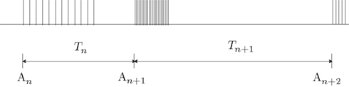
Figure 3. A scheme of a long time series of action potentials, composed of various regions that might differ from each other in the intensity of activity (e.g., firing rate). The time series is divided to epochs of activity; T_n, the duration of epoch n, might be different from, or equal to T_{n + 1}. A_n is the availability of channels at the beginning of the n-th epoch.

Neuronal adaptation: Graceful vs. Complex

Adaptation of neuronal response patterns to ongoing stimulation is usually thought of in monotonic terms; that is – the longer or more intense (frequency or amplitude) the stimulation series is, the neuronal responsiveness tends to gracefully reduce or gracefully increase, depending on the involved conductance, e.g. sodium or potassium, respectively. But there are reports in the literature, showing that adaptation to repeated stimuli may result in the emergence of intermittent, non-monotonic complex deterministic patterns of neuronal responses (e.g. Drew and Abbott, 2006; Gilboa et al., 2005; La Camera et al., 2006; Lowen et al., 1999; Manevitz and Marom, 2002; Tal et al., 2001). The following analysis offers an explanation that links the dimension of inactivation space of states, to the nature of adaptive neuronal responses to repeated stimuli.

Let us consider a simple case of Eq. 10, where T and Γ are constants – i.e., the case of periodic activations. Under these conditions Eq. 10 becomes:

where is the fraction that inactivates during an epoch, and . In what follows, for convenience, the tilde symbol is omitted from the parameter . The fraction inactivated during each epoch, Γ, contributes to the dynamics by linearly offsetting the map: as Γ increases, the slope of the map at A_n+1 = A_n becomes more negative, pushing the system towards instability and bifurcations. For 0 < D < 1, as D increases it acts as a “buffer” that defers the occurrence of bifurcations for any A < 1. In fact, the lower bound of Γ_critical for the occurrence of the first bifurcation of A goes to infinity as D approaches unity: The exact solution is arrived at by noting that at steady state (s), A_n+1 = A_n. Thus,

The first derivative of Eq. 11 in respect to A is

which goes to −1 at the first bifurcation point, where

Since , the resulting inequality reduces to

at 0 < c < 2; that is, where T is within the range of, or smaller than (the lower limit of recovery time scale), as D → 1, .

Figure 4 demonstrates the above point; it shows examples of bifurcation diagrams, computed by iterating Eq. 11 in a range of Γ at three different D values. Deterministic transitions between different values of A occur as a function of the fraction inactivated (Γ) at each generation. Note that the sensitivity of the dynamics to the activity depends on D: Where the space of inactivated states is small, the value of D is small and the diagram bifurcates at a relatively low inactivation rate. As the chain of inactivated states becomes longer, D increases and buffers the dynamics, deferring the first bifurcation point to higher inactivation rates. Thus, the existence of long chains of inactivation states protects the system from bifurcations, allowing for a wider range of graceful adaptation of the availability of channels over long time scales (black curve of Figure 4). Since we have mapped the dynamics of A to dynamics in the space of possible input–output relations, deterministic transitions between multiple values of A, such as the bifurcations in Figure 4, entail instability of input–output relations and enrichment of neuronal response patterns to a given stimulation regime. The manifestation of these dynamics of A in neural activity depends, of course, on the concept one has in mind for what a neural input–output function is. Yet, in general, it is safe to say that in the case of graceful adaptation (high D values), for each input frequency the system relaxes to one unique defined response mode; this is what the black curve of Figure 4 implies. Complex adaptation, that is bifurcation in the dynamics of A, means instability and non-monotonous exchange of response modes, for a given input frequency. This prediction of the model is strongly supported by measurements obtained in neural and cardiac preparations, as well as by concrete numeric simulations in which multiple timescales are manually introduced by additions of uniquely defined states and rates (e.g. Drew and Abbott, 2006; Gilboa et al., 2005; La Camera et al., 2006; Lowen et al., 1999; Manevitz and Marom, 2002; Soen et al., 1999; Tal et al., 2001); the strength of the present approach is in its simplicity: it shows that the dynamic range of adaptation in excitable membranes is reduced to a simple equation in which the essential non-linearity is replaced by a feedback loop between the history of activation and an adaptive transition rate that is sensitive to a single physiologically measurable dimension. Obviously, the continuous model of Eq. 8 can never lead to bifurcating response patterns of the kind seen in the above referenced studies. However, such complexity may be introduced when interacting populations of different ionic channels, expressed as coupled continuous equations, are considered (e.g. DeFelice and Isaac, 1993; Soen et al., 1999 and references therein).

FIGURE 4

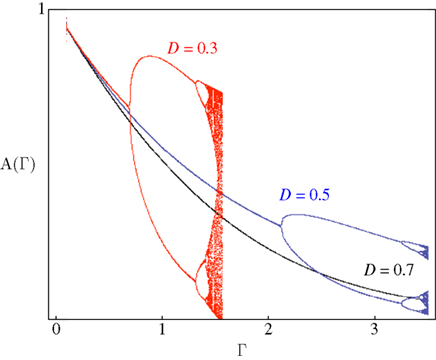
Figure 4. Bifurcation diagrams computed by iterating Eq. 11. Solutions for a range of Γ with three different D values are shown. Scaling to approximately cover the full range of solutions was achieved by setting c = 1.7.

Distribution of D, development and adaptation

In the above analyses of excitability dynamics, beyond the time scale of a single action potential, a significant emphasis is put on the value of D, the dimension of inactivated space of states; different values of D may cause very different long-term dynamics. As D increases, the system is less sensitive to high frequency fluctuations around its steady-state solution, and becomes less susceptible to bifurcating response modes. Experimental measurements show that D has a wide range in various types of channels. This supports the richness of dynamics observed in different types of cells, and changes in excitability within a given cell along its developmental timeline. For instance, Toib et al. (1998) reported D = 0.8 for NaII (the neonatal form of cortical neuron sodium channel), D = 0.5 for NaIIA (the adult form of cortical sodium channel), and D = 0.1 for the A-type ShakerB potassium selective channel; Ellerkmann et al. (2001) reported sodium conductance D values that range from 0.3 to 0.6 in hippocampal granule cells, hilar neurons and basket cells; Melamed-Frank and Marom (1999) reported D = 0.3 in the wild-type skeletal muscle voltage-gated Na channel (SkM1), but D = 0.6 in the SkM1 (T698M) mutant that is believed to cause Hyperkalemic periodic paralysis; Uebachs et al. (2006) reported scaling of recovery rates that is dramatically reduced in Ca(v)3.2 and Ca(v)3.3, but not Ca(v)3.1. These and related observations suggest that the dimensionality of the space of inactive states is a powerful modulator of excitability dynamics that depends on the patterns of prior activity; a time scale free mechanism for cellular plasticity that emerges from the biophysical properties of channel subunits.

Recapitulation

There is a tendency, in recent years, to model excitability by accounting for all possible measurable variables and parameters. Indeed, the measurement techniques become increasingly precise, computers become increasingly strong, and the present state-of-the-art (especially in the discipline of neuroscience) brings to mind Borges comment “On Exactitude in Science” (J. L. Borges, A Universal History of Infamy, Penguin Books, London, 1975; translated by Norman Thomas de Giovanni):

…In that Empire, the craft of Cartography attained such Perfection that the Map of a Single province covered the space of an entire City, and the Map of the Empire itself an entire Province. In the course of Time, these Extensive maps were found somehow wanting, and so the College of Cartographers evolved a Map of the Empire that was of the same Scale as the Empire and that coincided with it point for point…

The study described here takes a different (perhaps complementary) approach, by interpreting ion channel kinetics in terms of population dynamics. Notwithstanding obvious qualifications, it suggests that such an approach produces a mathematically tenable reduced model, which is based on a small number of experimentally measurable parameters, and with immediate physiological implications on our understanding of adaptation in excitable cells. The hope is that this approach will serve for analyses of excitability in point and extended systems; analyses that are realistic in the sense of dealing with the richness of molecular time scales, yet do not involve accounting for an ever-increasing number of molecular degrees of freedom. Current reduced models fall short in this respect.

Conflict of Interest Statement

The author declares that the research was conducted in the absence of any commercial or financial relationships that could be construed as a potential conflict of interest.

Acknowledgments

The author thanks E. Braun, N. Brenner, D. Dagan, D. Eytan, A. Gal, R. Meir and A. Wallach for encouragement and comments.

References

Bassingthwaighte, J., Liebovitch, L., and West, B. (1994). Fractal Physiology. New York, Oxford University Press.

DeFelice, L., and Isaac, A. (1993). Chaotic states in a random world: Relationship between the nonlinear differential equations of excitability and the stochastic properties of ion channels. J. Stat. Phys. 70, 339–354.

CrossRef Full Text

Drew, P. J., and Abbott, L. F. (2006). Models and properties of power-law adaptation in neural systems. J. Neurophysiol. 96, 826–833.

Pubmed Abstract | Pubmed Full Text | CrossRef Full Text

Ellerkmann, R. K., Riazanski, V., Elger, C. E., Urban, B. W., and Beck, H. (2001). Slow recovery from inactivation regulates the availability of voltage-dependent Na(+) channels in hippocampal granule cells, hilar neurons and basket cells. J. Physiol. 532(Pt 2), 385–397.

Pubmed Abstract | Pubmed Full Text | CrossRef Full Text

Fairhall, A. L., Lewen, G. D., Bialek, W., and de Ruyter Van Steveninck, R. R. (2001). Efficiency and ambiguity in an adaptive neural code. Nature 412, 787–792.

Pubmed Abstract | Pubmed Full Text | CrossRef Full Text

French, A. S., and Torkkeli, P. H. (2008). The power law of sensory adaptation: simulation by a model of excitability in spider mechanoreceptor neurons. Ann. Biomed. Eng. 36, 153–161.

Pubmed Abstract | Pubmed Full Text | CrossRef Full Text

Gilboa, G., Chen, R., and Brenner, N. (2005). History-dependent multipletime-scale dynamics in a single-neuron model. J. Neurosci. 25, 6479–6489.

Pubmed Abstract | Pubmed Full Text | CrossRef Full Text

Hille, B. (1992). Ionic Channels of Excitable Membranes, 2nd Edn. Sunderland, Sinauer Associates.

Hodgkin, A., and Huxley, A. (1952). A quantitative description of membrane current and its application to conduction and excitation in nerve. J. Physiol. 117, 500–544.

Pubmed Abstract | Pubmed Full Text

Jones, S. W. (2006). Are rate constants constant? J. Physiol. 571(Pt 3), 502.

Pubmed Abstract | Pubmed Full Text

Kleber, A. G., and Rudy, Y. (2004). Basic mechanisms of cardiac impulse propagation and associated arrhythmias. Physiol. Rev. 84, 431–488.

Pubmed Abstract | Pubmed Full Text | CrossRef Full Text

La Camera, G., Rauch, A., Thurbon, D., Luscher, H. R., Senn, W., and Fusi, S. (2006). Multiple time scales of temporal response in pyramidal and fast spiking cortical neurons. J. Neurophysiol. 96, 3448–3464.

Pubmed Abstract | Pubmed Full Text | CrossRef Full Text

Liebovitch, L. S., Fischbarg, J., Koniarek, J. P., Todorova, I., and Wang, M. (1987). Fractal model of ion-channel kinetics. Biochim. Biophys. Acta 896, 173–180.

Pubmed Abstract | Pubmed Full Text | CrossRef Full Text

Lowen, S. B., Cash, S. S., Poo, M., and Teich, M. C. (1997). Quantal neurotransmitter secretion rate exhibits fractal behavior. J. Neurosci. 17, 5666–5677.

Pubmed Abstract | Pubmed Full Text

Lowen, S. B., Liebovitch, L. S., and White, J. A. (1999). Fractal ion-channel behavior generates fractal ring patterns in neuronal models. Phys. Rev. E Stat. Phys. Plasmas Fluids Relat. Interdiscip. Topics 59(Pt B), 5970–5980.

Pubmed Abstract | Pubmed Full Text

Lundstrom, B. N., Higgs, M. H., Spain, W. J., and Fairhall, A. L. (2008). Fractional differentiation by neocortical pyramidal neurons. Nat. Neurosci. 11, 1335–1342.

Pubmed Abstract | Pubmed Full Text | CrossRef Full Text

Manevitz, L. M., and Marom, S. (2002). Modeling the process of rate selection in neuronal activity. J. Theor. Biol. 216, 337–343.

Pubmed Abstract | Pubmed Full Text | CrossRef Full Text

Markram, H. (2006). The blue brain project. Nat. Rev. Neurosci. 7, 153–160.

Pubmed Abstract | Pubmed Full Text | CrossRef Full Text

Marom, S. (1994). A note on bistability in a simple synapseless ‘point neuron’ model. Netw. Comput. Neural Syst. 5, 327–331.

CrossRef Full Text

Marom, S. (1998). Slow changes in the availability of voltage-gated ion channels: effects on the dynamics of excitable membranes. J. Membr. Biol. 161, 105–113.

Pubmed Abstract | Pubmed Full Text | CrossRef Full Text

Marom, S., and Abbott, L. F. (1994). Modeling state-dependent inactivation of membrane currents. Biophys. J. 67, 515–520.

Pubmed Abstract | Pubmed Full Text | CrossRef Full Text

Marom, S., and Levitan, I. B. (1994). State-dependent inactivation of the kv3 potassium channel. Biophys. J. 67, 579–589.

Pubmed Abstract | Pubmed Full Text | CrossRef Full Text

Melamed-Frank, M., and Marom, S. (1999). A global defect in scaling relationship between electrical activity and availability of muscle sodium channels in hyperkalemic periodic paralysis. Pflugers Arch. 438, 213–217.

Pubmed Abstract | Pubmed Full Text | CrossRef Full Text

Millhauser, G., Salpeter, E., and Oswald, R. (1988a). Diffusion models of ion-channel gating and the origin of power-law distributions from single channel recording. Proc. Natl. Acad. Sci. U.S.A. 85, 1503–1507.

CrossRef Full Text

Millhauser, G., Salpeter, E., and Oswald, R. (1988b). Rate-amplitude correlation from single-channel records. A hidden structure in ion channel gating kinetics? Biophys. J. 54, 1165–1168.

CrossRef Full Text

Murray, D. (1993). Mathematical Biology. Berlin, Springer.

Soen, Y., and Braun, E. (2000). Scale-invariant fluctuations at different levels of organization in developing heart cell networks. Phys. Rev. E Stat. Phys. Plasmas Fluids Relat. Interdiscip. Topics 61, R2216–R2219.

Pubmed Abstract | Pubmed Full Text | CrossRef Full Text

Soen, Y., Cohen, N., Lipson, D., and Braun, E. (1999). Emergence of spontaneous rhythm disorders in self-assembled networks of heart cells. Phys. Rev. Lett. 82, 3556–3559.

CrossRef Full Text

Tal, D., Jacobson, E., Lyakhov, V., and Marom, S. (2001). Frequency tuning of input–output relation in a rat cortical neuron in-vitro. Neurosci. Lett. 300, 21–24.

Pubmed Abstract | Pubmed Full Text | CrossRef Full Text

Teich, M. (1989). Fractal character of the auditory neural spike train. IEEE Trans. Biomed. Eng. 36, 150–160.

Pubmed Abstract | Pubmed Full Text | CrossRef Full Text

Toib, A., Lyakhov, V., and Marom, S. (1998). Interaction between duration of activity and time course of recovery from slow inactivation in mammalian brain Na+ channels. J. Neurosci. 18, 1893–1903.

Pubmed Abstract | Pubmed Full Text

Turrigiano, G., Marder, E., and Abbott, L. (1996). Cellular short-term memory from a slow potassium conductance. J. Neurophys. 75, 963–966.

Uebachs, M., Schaub, C., Perez-Reyes, E., and Beck, H. (2006). T-type Ca2+ channels encode prior neuronal activity as modulated recovery rates. J. Physiol. 571(Pt 3), 519–536.

Pubmed Abstract | Pubmed Full Text