Self-organized critical noise amplification in human closed loop control

Introduction

Physical behavior in the world is confronted with the ongoing changes of the body as well as the controlled situation. For instance, muscles fatigue and environmental conditions may vary rapidly. While the dynamics of a given closed loop control situation could be known by the nervous system, for example, by previous learning over long periods of time, the actual parameters permanently need to be adjusted on-line. In other words, brains realize adaptive control in non-stationary closed loop situations. Here, we investigate the consequences of rapid adaptivity for the dynamics of motor control in theory, simulations, and human experiments.

Many complex systems exhibit non-Gaussian fluctuations of state variables x with distributions P(x) that are well described by P(x) ∝ x^−δ (δ< 0) for large magnitudes. Examples include sizes of avalanches of granular matter, the distribution of earthquake magnitudes (Gutenberg–Richter law) and stock-market log-return fluctuations (Sornette, 2004 ). Recently, theoretically predicted power law distributions (Eurich et al., 2002 ) were experimentally found (Beggs and Plenz, 2003 ) also in the firing behavior of neural populations in cortical tissue.

Scaling behavior has also been identified in human sensory-motor control systems such as the balancing of a stick at the fingertip (Cabrera and Milton, 2002 ; Cabrera et al., 2004 ) and the visuomotor control of a virtual target on a computer screen (Bormann et al., 2004 ). Generally, scaling of fluctuations is indicative of scale invariance of the considered system's dynamics. In physics, this occurs in extended systems close to a phase transition (bifurcation), that is, when a system is in a critical state. Alternatively, the system could also be close to intermittency, which in the case of stick balancing has been suggested as the reason for the occurrence of power law tails (Heagy et al., 1994 ) where it was argued that it results from the existence of multiplicative noise and a fine-tuning of system parameters to a stability boundary (Cabrera et al., 2004 ).

A problem with these explanations is their dependency on parameters; power law behavior emerges only when they are carefully adjusted, in other word, the criticality in these models is not generic. Critical dynamics could in principle also emerge from the so-called self-organized criticality (SOC) (Bak et al., 1987 ), a mechanism by which high-dimensional systems may settle into critical states instead of evolving toward equilibria. While this phenomenon might be relevant for some neuronal systems (Levina et al., 2006 ), it is not clear how SOC might be involved in control performed by the human nervous system.

Here, we discuss a control mechanism that yields critical behavior without the need of parameter tuning or high dimensionality. Since real world situations are non-stationary, we are particularly interested in a controller with finite memory that uses only few past observations for estimation. Previously, we already showed that optimal on-line adaptation of a controller using finite memory generically leads to a critical situation which entails power-law-fluctuations (Eurich and Pawelzik, 2005 ). Furthermore, we investigate if human behavioral control might originate from such critical noise amplification by performing experiments with humans in a control situation which closely matches the conditions of the theory. We include realistic constraints in the model and investigated their influence on the dynamics of the overall system. By matching characteristic statistical properties of the dynamics of the model to the experiments, we determine basic parameters governing the control dynamics of individual subjects.

Materials and Methods

Basic model

A time-discrete random map

defines a control problem where the dynamical variable y_t denotes the deviation of a system from some target value at time t(t = 0, 1, 2,…). α⁰ is a system parameter unknown to the controller and assumed to be constant for at least some period of time. For α⁰ > 1, the fixed point at the origin is linearly unstable. is a Gaussian random variable describing non-predictable fluctuations. Its variance σ² ≡ const. is a second hidden system parameter.

The controller is assumed to know the form of the dynamical Equation (1). The strategy consists in computing an estimate α_t of the parameter α⁰ from previous observations y_t, y_t−1,…of the system. The controller uses this estimate and the observed previous deviation y_t to remove the term α_t y_t which corresponds to the predicted next deviation from the target. When control is switched on, Equation (1) is replaced by

In the following, we employ a minimum mean squared error approach for a controller's estimation of the control parameter α⁰, that is, where the brackets denote the expectation with respect to the additive noise. The expectation value of the squared deviation from the target is

For simplicity, we here assume that only the observable values of y_t and y_t−1 are taken into account by the controller and we use

(obtained from rearranging Equation (2) where we replaced t by t−1) to eliminate α⁰ in Equation (3). It is now straightforward to minimize Equation (3) with respect to α_t by setting

which yields the optimal estimator for α_t from the two very recent observations:

Equations (2) and (6) represent the dynamics of the basic adaptive control system as a two-dimensional map. By inserting the right-hand side of Equation (2) into Equation (6), the estimator can be written in the form

This form of the equation shows that the estimated value of the system's parameter becomes dominated by the noise β_t when y_t has small values. In the Results Section, we present a proof that this mechanism generically leads to power law distributed y independently of α and the noise level.

A simple control experiment

We investigated control behavior of humans in a simple balancing task. A target and a cursor were presented on a computer screen. The x- and y-components of the target position T moved according to

and the cursor position M was controlled by the subjects using a computer mouse. The task of the subjects was to stabilize the target by moving M as close to T as possible. This situation is for each component equivalent to the basic control problem described above if the controller would move the cursor to the target prediction which defines his estimation of the control parameter α_t. Subtracting on both sides in Equation (8) then yields Equation (2) with . Furthermore, we assumed that the noise β_t in the experiment is realized by noise inside the brain and the motor system controlling the hand guiding the mouse.

The computer was a PC with 1800 Mhz and 512 MB working memory, a graphics card with a GeForce FX chip set and 64 MB memory, an USB computer mouse with 800 dpi resolution and a sampling rate increased to its maximum of 500 Hz, and a 19 inch color monitor with 85 Hz and resolution of 1280 × 1024 pixels. The movement of the mouse was constrained to a low friction glass mouse pad of 25 × 30 cm² size. Target and mouse were presented on the screen as rectangles of 5 pixels side length. The program controlling the experiments was designed to nearly achieve real-time processing. Operating system was Linux Fedora Core 3 (Version 11∕2004) with real-time capability provided by the RTAI 3.1 package (http://www.rtai.org ). Movement of target and cursor was controlled by a program written in C using OpenGL as a graphical frontend. Real time operation of this system was verified, occasional time errors were of the order of 2 ms.

Seven subjects participated in the experiments, filled a questionnaire according to the ethical requirements of human experimentation, and declared their informed consent. The subjects were of ages 21 to 59, right-handed and one subject was female. During experiments, each subject was positioned 60 cm in front of the screen in a closed room without window, which was only weakly lighted from the back. During a trial, two circles were presented on the screen: a green one (M) for the mouse and a one red (T) for the target (Figure 1 ). M was moved linearly proportional to the position of the subjectquotidns hand using the mouse, limited by the screen border. 10 millimeter mouse movement corresponded to 445 pixels. Temporal resolution of the mouse was 2 ms and its spatial resolution corresponded to 1.41 pixels. Task was to keep M and T together as close as possible without one of them running out of the screen, a situation similar to balancing a stick on the tip of a finger. A trial was started by pressing a button on the keyboard and began with M and T being placed in the middle of the screen.

FIGURE 1

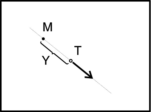
Figure 1. Control of a virtual target T (circle) on a computer screen (rectangle) by movements of a computer mouse M (black dot). The arrow indicates that the movement of the target depends on the relative position of T and M.

The parameter α⁰ was chosen larger than one. Thereby, M represents an unstable fixed point of the dynamics of T. The larger α⁰, the more difficult was the task. Subjects 1, 2, and 3 performed the tasks with α⁰ = const., for the others α⁰ was randomly switched every second to a value in {3, 4, 5, 6}.

During a trial, the x- and y-positions of mouse and target were recorded as events with a frequency that was coupled to the refresh rate of 85 Hz of the screen. A trial ended if either one of the points left the screen or the maximal recording time of 3 minutes had expired. Before the subsequent trial a break of 5 minutes allowed for relaxation. At least 15 trials per day were recorded. Experiments were authorized by the ethics committee of the University Bremen.

Realistic constraints

An application of our therory to realistic systems (such as the balancing of a stick or human postural sway) will only be possible if the mechanism of generating power law behavior in the model is robust with respect to the introduction of delays, memory, and changes in the dynamics of the controlled system. Here, we introduce two extensions: delay and memory.

Interaction delays are ubiquitous in motor control (e.g., Cabrera and Milton, 2002 ; Cabrera et al., 2004 ; Eurich and Milton 1996 ; Woollacott et al., 1998 ). One can introduce a delay n = 0, 1, 2, …to shift the observations used for estimation further into the past. Then, Equation (6) is replaced by

which will be referred to as system with delay n. Note that due to causality an application of the basic model to the experimental situation requires a delay of n > 0.

A second extension of the basic model takes into account more past observations than only y_t and y_t−1, that is, a longer memory. For the basic model, we derived the control Equation (6) by minimizing the mean square error of the estimator. This is equivalent to maximizing the likelihood of the predicted target position. It is straightforward to expand this approach to a longer memory by using the joint probability density (Eurich and Pawelzik, 2005 ):

Evaluation of this equation yields the optimal estimation of α₀ when m past observations are considered additionally to the two steps used for the basic model. In this case, the estimation equation reads

To make this extension biologically more realistic, exponentially decaying weights e^−i∕τ with time constant τ can be assigned to the summands in the numerator as well as in the denominator to replace the artificially box-shaped memory (10) by an exponentially fading one. Taking the limits m →∞, this leads to a set of estimation equations with exponentially decaying memory

Together with Equation (2), these equations represent a biologically more plausible version of a closed loop control system with only two parameters: εand n. For ε =1, these equations are equivalent to the basic control system without memory and for ε =0, the memory becomes infinite. The characteristic decay time of the memory is τ =− ln(1 −ε)⁻¹, which becomes τ ≈1∕ε for small ε.

Finally, the control Equation (11) could also be equipped with constraints to suppress unrealistically large estimates of α⁰, for example, by adding a small positive term to B_t. We found that also this extension of the system yields power law tails of p(y_t) which, however, then have an exponential cutoff. Because the inclusion of such a truncation complicates the systemquotidns dynamics without providing substantial benefits for the following discussion, it will not be considered here.

Simulations

For comparison with the experimental data, datasets of the basic model and of the model with exponentially decaying memory have been generated. These datasets comprised 10⁶ iterations and parameters were α⁰ = 2, σ² = 0.8. The realistic model had a delay of n = 10 steps and a memory with parameter ε =0.85. These datasets have been analyzed analogously to the experimental data sets (Figures 2 and 4 ).

FIGURE 2

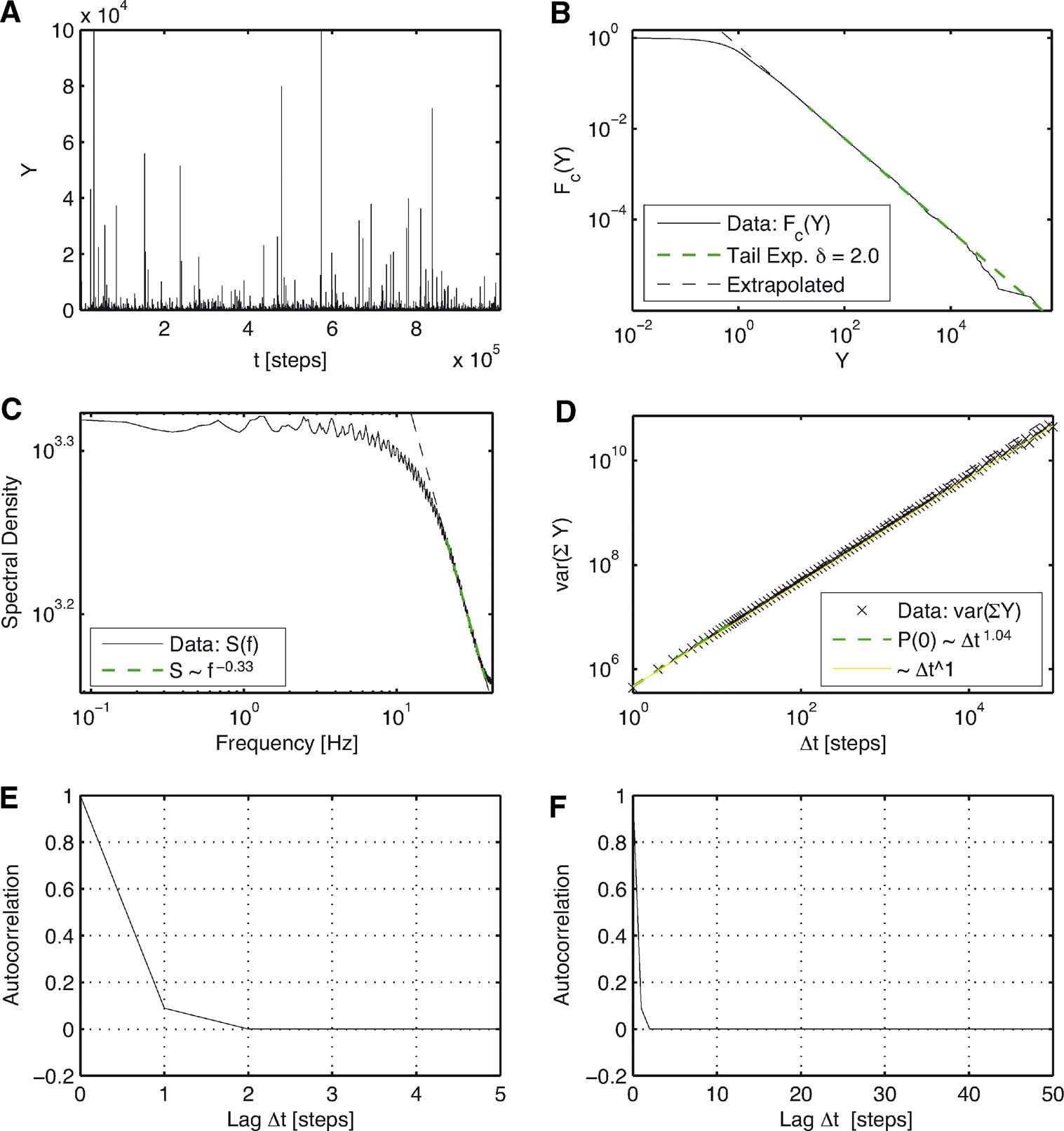
Figure 2. Results for the basic model. (A) Time series of the distances Y = |y| versus iteration steps. (B) Complementary cumulative distribution function of Y. The linear dependency observed in double logarithmic presentation exhibits clear power law behavior for large Y with a corresponding exponent δ =2.0 as predicted analytically (24). (C) The power spectrum for large frequencies scales with exponent 0.33. For low frequencies, it is constant. (D) The variance of the cumulated magnitudes scales with a Hurst exponent close to 0.5. (E), (F) Autocorrelation of Y on different lag ranges. Contrary to intuition, no anti-correlation occurs.

To further examine the dependence of the probability density tail exponent on the parameters of the system defined by Equations (2) and (11), time series have been simulated for different combinations of n and ε (Figures 5 and 6 ). To reduce statistical fluctuations in the tails, the rank-ordered absolute values of |y| from 10 simulations with 10⁹ iterations each have been averaged. Then, the tail exponents have been calculated using the Hill estimator as described in the following section. In one series of simulations (Figure 5 ), the parameters were fixed to α =2 and σ² = 0.8. In a second one (Figure 6 ), α⁰ was randomly chosen from {2, 3, 4} every 30 time steps. Using very long time series also helps fitting densities with very high tail exponents, because these tend to have a very slow transition with a low curvature leading to the power law regime.

Data analysis

Both experimental and simulated data were analyzed with different statistical methods. To obtain better statistics, the repeated trials of the participants from day 1 were combined into one time series with a length of some 10⁵ events.

Because the experimental task was to align mouse and target on a two-dimensional computer screen, the resulting data has two components for both, the positions of mouse and target. The differences

are the distances between mouse and target in the x - or y-direction on the screen in pixel units at time t. Since the axes of the screen represent an artificial coordinate system, it seems unlikely that the separate representation in x- and y-position is of any meaning to the brain. For that reason, we focused on the Euclidean radial distance between mouse and target

The main difference between the distance and the differences in the components is, that Y is always positive. However, we found that the radial distance and the absolute values of the differences in the components have almost identical statistical properties (not shown). Since the probability distributions of the components of the differences are symmetric, the positive part and the mirrored negative part of the difference distributions and the distributions of the absolute values of the distances overlap perfectly.

To compare the simulated time series with the experimental ones, the absolute values of y have been analyzed analogously to Y. In the following, we will refer only to the distances Y where for the simulated data |y| is implied.

Estimating parameters of distributions of rare, extreme events in general is quite difficult and therefore has to be done carefully. We obtained the tail exponents for the probability distributions by using the maximum likelihood estimator for rank-ordered distances Y known as “Hill estimator” (Sornette, 2004 ). This estimator uses the first r ranks, which correspond to the largest events up to a cutoff rank r. Smaller events which may belong to a different regime are discarded. This method takes into account the strong statistical fluctuations in the largest events and has therefore the advantage of being mathematically well founded, requiring only one cutoff, and no binning. This estimator is sensitive to the cutoff because the beginning of the power-law regime varies between trials and simulations with different exponents. To estimate the optimal cutoff, the exponents for 100 different logarithmically spaced cutoffs are calculated. For time series of the order of 10⁵ to 10⁶ steps, like the experimental datasets and the simulations analyzed for comparison, it turned out that the first 45% and the last 30% of the log of the range of the ranks can be regarded as not being well suited as a cutoff rank, which therefore has to lie within this range. For the larger and averaged simulations (Figures 5 and 6 ), these restrictions on the cutoff could be relaxed, since the criterion used to determine the cutoff could not be fooled by random bumps or kinks. The exponent of the fit with a cutoff in the relevant range and the least square error per rank is regarded as being optimal. This method has been tested on all datasets from whole days as well as from all single trials and from the simulated data. It turned out to provide reasonable results for all but few very crooked experimental distributions. Another method we tested was to search for the minimum of the slope of the estimated exponent when varying the cutoff. This method on average delivers results consistent with the first method, but is less robust and is therefore not considered in the following.

Results for experimental data and simulations are presented in Figures 2 through 6 and summarized in Table 1 . In Figures 2 , 3 and 4 , the respective six subplots show:

1. The time series Y plotted over the time measured in seconds or steps.
2. The complementary cumulative distribution function F_c(Y_t) = P(Y > Y_t) plotted in double logarithmic axes. The exponents δ of the tails of the probability densities of Y have been calculated using the Hill estimator as described above. Note that the exponent μ from the complementary cumulative distribution functions is related to δ as μ =δ− 1.
3. Power spectrum of Y. To reduce noise, for the combined time series from day 1, the time series is divided into 10 parts for each of which the power spectrum is computed individually. These 10 spectra are then averaged. The resulting spectrum has a lower noise level at the cost of raising the lowest frequency representable. Since the power spectrum is constant for low frequencies, the number of parts has been selected to obtain more information on the decay at high frequencies at the cost of the low frequencies. For the simulated time series, power spectra of 10³ parts are averaged.
4. Scaling of the variance of the sums of subsequent values of Y. For i.i.d. random variables with finite variance, it scales with the number n of summands as n^2H = n (random walk), where H is the Hurst exponent.
5. and F. Autocorrelation function of Y plotted against the lag.

In all sub-plots, green and cyan colored lines mark the fitted part while black lines are extrapolations. Fits in sub-plots C to F have been obtained using the method of least square errors.

TABLE 1

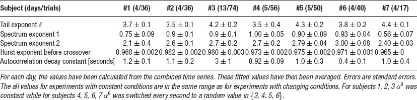
Table 1. Mean of the exponents δ of the distributions of |Y|, of the exponents of both regimes of power-law scaling in the spectral density, of the Hurst exponents and characteristic decay constants of the autocorrelations for the different subjects.

Results

Self-organized critical control

The simple map (Equations 2 and 6) generates time series which exhibit power law distributions of Y (Figure 2 ). While this controller is optimal in the sense that it uses the minimum mean squared error estimate of the systemquotidns parameter α⁰ from two past observations, the large fluctuations indicate that the system is sub-optimal from a global perspective when the control is rather successful, that is, when the values of y_t become small. Intuitively, for small amplitudes estimating the parameters does not make sense because the dynamics is then dominated by the noise. In other words, a controller with unlimited sensitivity will always run into the point where its estimate fits only the noise. In this sense, our simple model system exhibits self-organized criticality.

The power law behavior of the basic system for large fluctuations can be determined from an analytical treatment. Starting point is the iterative equation

which follows from our control equations if we insert the controller into the dynamics. For the formal solution of the density P(y), we have the general equation

The conditional probability density is given by the dynamics

where δ is the Dirac Delta distribution. The joint density is obtained from marginalization over the densities P(y) and P_β(β)

After integrating over β_t−2, this does not look too bad,

Putting everything together, we then have

Next, we integrate over y_t because it appears only in two of the Gaussian densities. We obtain

Now we integrate over y_t−1 which appears in P and as its reciprocal in one of the Gaussian densities. It is straightforward to estimate this integral for very large y which finally yields

and proves that the asymptotic exponent is −2. This requires that the desired distribution P(x) is finite for small arguments x (which is heuristically obvious and a numerical fact). Namely, with f(x) = const. for x → 0 and y large compared to the variance of a Gaussian density g we have the general relation

The remaining integrals exist and do not depend on y. Therefore, they contribute only a constant factor in Equation (23).

Numerical investigations indicate that for the system with memory m(Equation (10)) and no delay, the probability density has a tail exponent , independently of the value of α⁰ and the constant noise level (not shown).

Complex dynamics of human control behavior

Figure 3 shows statistics of subject 4 on his third day of measurement. Similar results were obtained for all subjects. The experimental data show similarities as well as differences to the basic model.

In particular, for all subjects, a power law is found in the probability densities. In individual trials, most tail exponents are between three and five. An average autocorrelation decays quickly to zero and does not become significantly negative. In single trials, anti-correlations occur which, however, are always within the noise range. The power spectrum is constant for low frequencies and then exhibits two regimes of power law decay which are more distinct for some trials than for others. The scaling of the variance for the sums of values of Y exhibits a Hurst exponent H > 0.5 for short times. A crossover to a Hurst exponent close to 0.5 occurs where the sums are over times of the order of few seconds. The results for all subjects are summarized in Table 1 .

Influence of constraints

Figure 4 shows the results from analyzing the extended model (Equations 2 and 11) for a choice of parameters that give results similar to the experimental data in Figure 3 .

FIGURE 3

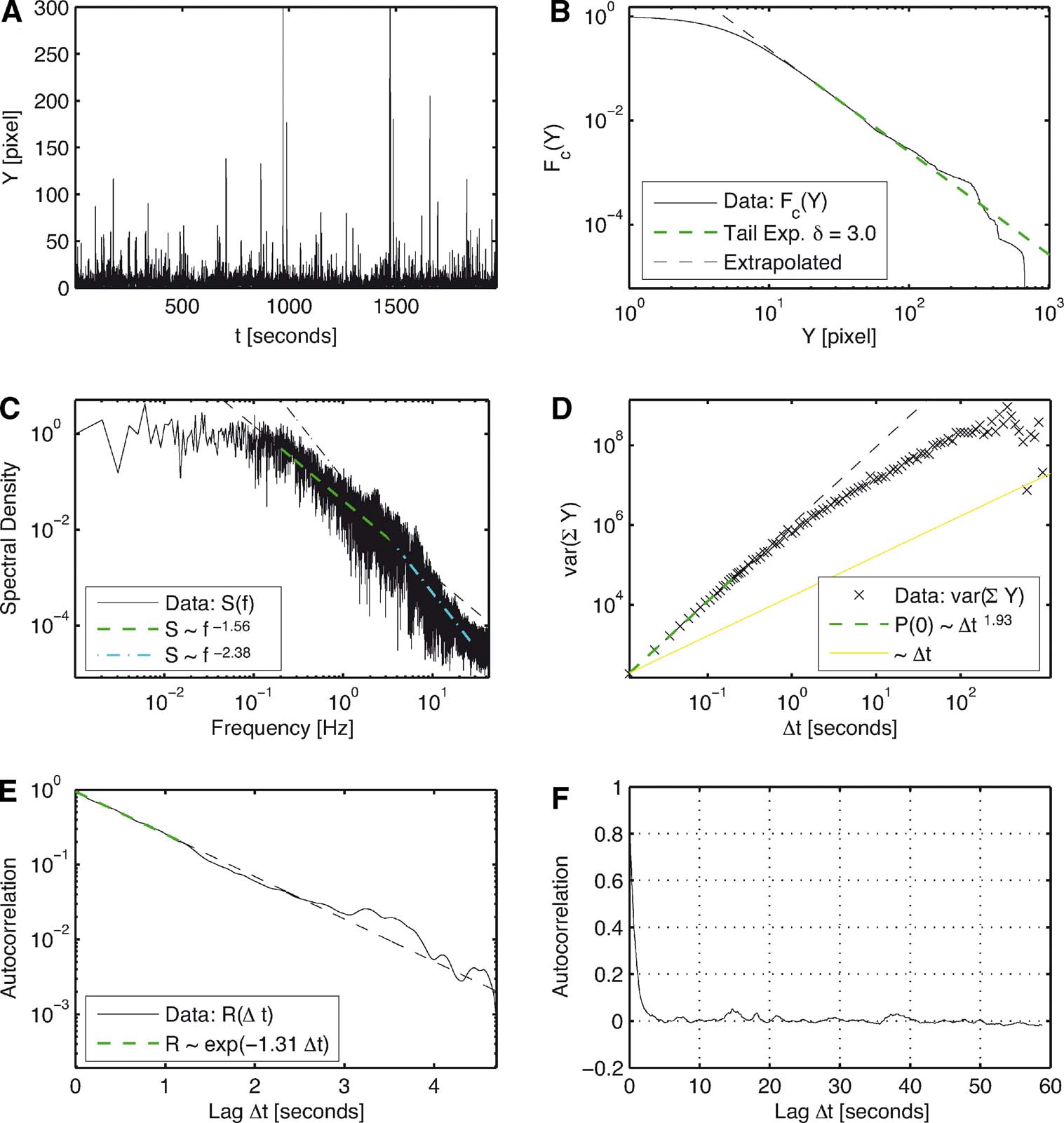
Figure 3. Analysis of the combined time series from day 3 of subject 4. (A) Time series of the distances Y over iteration steps. (B) Complementary cumulative distribution function of Y. The linear behavior in double logarithmic scaling exhibits clear power law behavior for large Y with a corresponding exponent of δ =3.0 in P(Y). (C) The power spectrum for large frequencies initially scales with exponent 1.56 and then with an exponent 2.38. For low frequencies, it is constant. (D) Variance of the cumulated magnitudes scales with a Hurst Exponent of H = 1.0 and then evolves to a Hurst exponent close to 0.5. (E) The autocorrelation of Y shows an exponential decay for short lags. (F) It quickly decays to zero without overshoot.

The exponent depends on the memory available to the controller. Larger memory leads to larger exponents, while long delays reduce the exponents. A controller with no memory and positive delay leads to tail exponents smaller than 2. The power spectrum is always constant for low frequencies and shows a power law decay over one to two orders of magnitude at high frequencies. For some parameter combinations, the power spectrum shows two regimes with different exponents, in particular when the memory and the delay are sufficiently large. The autocorrelation decays very quickly. Anti-correlations of the order of −0.1 occur for simulations with small ε (large memory) and short delays. For longer delays, anti-correlation is strongly suppressed and would not be visible in more noisy data. Using a varying α⁰ throughout the simulation effectively supresses all anticorrelations. Varying the model parameters makes it possible to closely match each property of an experimental time series individually, while generating data which shares all properties of a given experimental time series at the same time turned out to be difficult. But even for different simulations with the same parameters, the generated time series may have varying properties due to random fluctuations. In Figure 4 , we chose the parameters to quantitatively match the scaling exponent of Figure 3 in the distribution of Y while achieving close qualitative matching in other features. Nevertheless, comparison with Table 1 shows, that these features are quantitatively still close to the range observed in the experimental data.

FIGURE 4

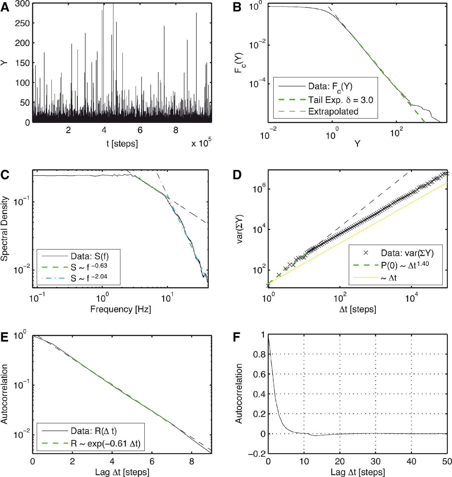
Figure 4. Simulation of the extended model with a delay of n = 10 steps and memory with ε =0.85. These parameters lead to statistical properties that qualitatively resemble the properties of the experimental data. (A) Time series of the distances Y = |y| over iteration steps. (B) Complementary cumulative distribution function of Y. The linear dependency in double logarithmic scaling exhibits clear power law behavior for large Y with a corresponding exponent δ =3.0 in P(Y). (C) The power spectrum for large frequencies initially scales with exponent 0.63 and then with an exponent 2.04. For low frequencies, it is constant. (D) Variance of the cumulated magnitudes scales with a Hurst Exponent of H = 0.7 and after 10 steps it then evolves to a scaling behavior with a Hurst exponent close to 0.5. (E) The autocorrelation of Y shows an exponential decay for short lags. (F) The autocorrelation quickly decays to zero and shows only very marginal anti-correlation.

To get an impression of the parameter dependence of the tail exponent δ of the distribution of the distances Y, Figure 5 shows δ versus memory length and delay. To examine the influence of non-stationary circumstances, Figure 6 shows the same representation but for the case of varying α⁰. For the static situation, the exponent rises monotonically with memory length while for varying α⁰, a long memory can be disadvantagous and reduces the exponent. To suppress large errors, the memory used by the controller has to be chosen according to the delay and the time scale of variation of the system to be controlled.

A reduction of the exponent for a longer memory even occurs, when the rate at which α⁰ changes is very low compared to the delay length. The worst case for the controller is when α⁰ is constant over a time interval being exactly as long as the delay time. This situation yields exponents much below 2 that rise again, when α⁰ is changed in periods being shorter than the delay time (not shown). This effect could allow to determine the delay experimentally. In these simulations, the controller was still able to control the system, because α⁰ was varied only over a limited range. This corresponds to the experiments, where the possible values for α⁰ were chosen in a range where the subjects where still able to stabilize the target. However, in different simulations the controller could handle much stronger variations in α⁰ when the intervals in which α⁰ stayed constant where longer than the delay, than in simulations, where these intervals where shorter than the delay.

FIGURE 5

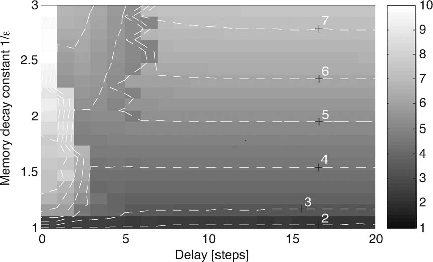
Figure 5. Tail exponent δ for different combinations of delay and decaying memory. Fitted using the Hill estimator, as described in Subsection Data Analysis. The rank-ordered absolute values of Y have been averaged for 10 simulations with 10⁹ time steps each with α⁰ = 2 and σ =0.8. For a fixed delay larger than 6, the exponent increases monotonously.

FIGURE 6

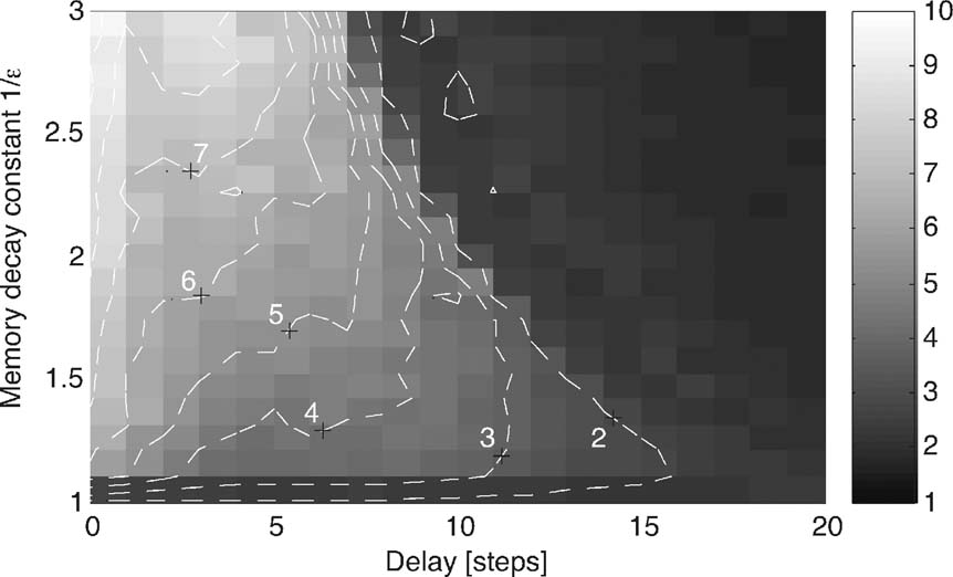
Figure 6. Tail exponent δ for simulations with parameter ranges as in Figure 5 , but with α⁰ chosen randomly from {2, 3, 4} every 30 time steps. In the presence of a delay, the exponent initially grows when increasing the memory length and decreases again for longer memories.

Summary and Discussion

Criticality emerges naturally in adaptive control by a very simple and intuitive mechanism: in the balanced situation, a systemquotidns parameters cannot be determined from its observable behavior because the system is then dominated by noise. In other words, the better the control, the less can be learned about the system. A controller with strictly limited memory who continuously estimates the parameters of an unstable system also when reasonable balance is already achieved thereby can run into catastrophic instabilities (MacArthur, 1995 ).

We analyzed this basic effect for a simple stochastic map. A controller using optimal on-line estimation from only two past observations was derived from minimizing the mean squared error. The resulting dynamics exhibit clear power law tails with an exponent δ =2 that was confirmed analytically. As can be seen from Equation (7), two mechanisms contribute to this behavior: first, the dynamical variable y_t appears in the numerator, resulting in large amplitudes if the controller has previously been successful in reducing the control error y_t to near zero. Second, the noise term is multiplicative. Multiplicative noise is well known to produce on-off intermittency and power law scaling in random maps (Heagy et al., 1994 ). Whereas previous models for motor control explicitly incorporated multiplicative noise (Cabrera and Milton, 2002 ), in our model it results from optimal parameter estimation of a simple linearly unstable system with additive noise coupled to a controller. Together with the fact, that power law behavior per se does not depend on the parameters and therefore is generic, this justifies the adjective “self-organized.” This criticality is in strong contrast to the usual SOC (Bak et al., 1987 ), in which a high dimensional system tends to be close to a bifurcation point. In our case, few coupled maps are sufficient which self-organize the state toward a point of maximal noise-sensitivity.

We investigated whether our theory can explain human motor control dynamics by performing experiments where subjects were asked to balance an unstable target on a screen with a cursor controlled using a computer mouse. Experiments were designed to closely match the conditions of the theory. For all subjects, target–mouse distance distributions strongly deviated from Gaussians and had tail exponents in the range of 2.5–6 (Table 1 ). The distance dynamics was correlated for seconds (Figure 3 E and 3 F), with Hurst exponents H > 0.5 for short times.

The basic model does not reproduce the features of human motor control dynamics (Figure 2 ). Correlations were very short, H = 0.5 for all times and the power spectrum did not exhibit two separate scaling-regions. This result a posteriori justifies the use of power spectra and scaling behavior of variances as decisive measures for testing models of control dynamics. To improve the correspondence with the experimental data, we extended the model to include exponentially fading memory, limitations on the ranges of estimated parameters, and the presence of delays. The occurrence of power law behavior was found to be robust with respect to delays, size of memory, noise level, and cut-offs of amplitudes. It turned out that the exponents δ >2 of the distribution's tails increase for long memory and decay with delay (Figure 5 ). Choices of the two-time constants for memory and delay that match the tail exponents of the trials from one day could reproduce slower decaying correlations and values of H > 0.5 with crossover to H = 0.5. (Figure 4 ). We found it particularly surprising that our models can match human control dynamics in so much detail despite the fact that the sensory-motor system is complex, involves many neuronal networks from motor cortex to spinal cord, and is subject to many physical constraints, as, for example, limits on muscle force and the inertia of the arm. We believe, however, that these constraints affect mostly the shape of spectrum and correlation, but do not strongly alter the scaling behavior of Y. Taking the parameters of the model seriously suggests that the memory for on-line adaptation is rather short (less than a second), while the delay for applying new estimates of the systems parameters is rather long (several seconds). Suprisingly, we found that control also works when the parameter α⁰ is switched in shorter intervals than the delay time, if the range of variation is limited.

We will soon test these predictions about the on-line adaptivity realized by the human motor control system in independent experiments. Also, we will perform experiments which independently measure delay and memory which will serve as a critical test of our model.

Taken together our results suggest that the human nervous system employs adaptive motor control using only a very limited memory of past observations for estimating the parameters of the controlled system. Fast adaptation is a prerequisite for survival in a non-stationary world. The fact that the consideration of a longer history yields faster decaying densities suggests that power laws observed in sensory-motor control result from a compromise between stability and fast adaptation with respect to changes in system parameters.

Clearly, our model is a black box explanation which calls for a microscopic realization in terms of neurons, synapses, and the like. While this is work in progress, we found it striking that the simple theory derived from optimality principles after inclusion of general constraints was able to reproduce the qualitative features of the dynamics. Our future work, both theoretical as well as experimental will put more flesh to the statements of the theory in order to clarify how a cortical network might realize estimation of system parameters for control, and how the properties of its elements (synapses, neurons, spinal chord, muscles, inertia of the arm, etc.) contribute to the constraints.

Our work might have some potential for explaining non-Gaussian behavior also of other systems with similar features in their dynamics. For instance, financial markets can be considered systems that optimize the dynamics of prices such that no trader possessing the available information can expect to achieve profit (Cherdron and Pawelzik, 2007 ). This can be considered a control situation and we are currently exploring the possibility that also here self-organized critical control underlies the stylized statistical features of price fluctuations (Mantegna and Stanley, 2000 ).

Conflict of Interest Statement

The authors declare that the research was conducted in the absence of any commercial or financial relationships that could be construed as a potential conflict of interest.

Acknowledgements

We thank Stefan Bornholdt, Christian Eurich and Misha Tsodyks for useful discussions, Misha Tsodyks also for help with the analytical treatment of the basic control system. This work has been supported by the German Ministry of Education and Research (BMBF, DIP Metacomp project) and benefited from a sabbatical visit of K.P at the Weizmann Institute.

References

Bak, P., Tang, C., and Wiesenfeld, K. (1987). Self-organized criticality: an explanation of 1∕f noise. Phys. Rev. Lett. 59, 381–384.

Pubmed Abstract | Pubmed Full Text

Beggs, J. M., and Plenz, D. (2003). Neuronal avalanches in neocortical circuits. J. Neurosci. 23, 11167–11177.

Pubmed Abstract | Pubmed Full Text

Bormann, R., Cabrera, J. L., Milton, J. G., and Eurich, C. W. (2004). Visuomotor tracking on a computer screen–an experimental paradigm to study the dynamics of motor control. Neurocomp. 58–60, 517–523

Cabrera, J. L., and Milton, J. G. (2002). On-off intermittency in a human balancing task. Phys. Rev. Lett. 89, 158702.

Pubmed Abstract | Pubmed Full Text

Cabrera, J. L., Bormann, R., Eurich, C. W., Ohira, T., and Milton, J. G. (2004). State-dependent noise and human balance control. Fluct. Noise Lett. 4, L107–L117.

Cherdron, U., and Pawelzik, K. (2007). Proceedings DPG spring meeting Regensburg 2007. Verhandl. DPG(VI) 42, 4∕AKSOE 13.2 (2007)

Eurich, C. W., and Milton, J. G. (1996). Noise-induced transitions in human postural sway. Phys. Rev. E 54, 6681–6684.

Pubmed Abstract | Pubmed Full Text

Eurich, C. W., Herrmann, J. M., and Ernst, U. A. (2002). Finite-size effects of avalanche dynamics. Phys. Rev. E 66, 066137.

Pubmed Abstract | Pubmed Full Text

Eurich, C., and Pawelzik, K. (2005). Optimal control yields power law behavior. In ICANN 2005, LNCS 3697, W. Duch et al., eds. (Berlin, Heidelberg, Springer-Verlag), pp. 365–370.

Heagy, J. F., Platt, N., and Hammel, S. M. (1994). Characterization of on-off intermittency. Phys. Rev. E 49, 1140–1150.

Pubmed Abstract | Pubmed Full Text

Levina, A., and Herrmann J., M. (2006). Dynamical Synapses give rise to a power-law distribution of neuronal avalanches. Advances in Neural Information Processing Systems 18, Y. Weiss, B. Schölkopf, and J. Platt, eds. (Cambridge, MA, MIT Press), pp. 771–778.

MacArthur, J. (1995). ‘Air Disasters 1’. (Fyshwick, Australia, Aerospace Publications Pty Ltd), pp. 22–29.

Mantegna, R. N., and Stanley, H. E. (2000). An introduction to econophysics (Cambridge, UK, Cambridge University Press). ISBN 0 521 62008 2.

Sornette, D. (2004). Critical phenomena in natural sciences: chaos, fractals, selforganisation and disorder: concepts and tools, 2nd edn (Berlin, Heidelberg 2000, 2004, Springer-Verlag) ISBN 3-540-40754-5.

Woollacott, M. H., von Hosten, C., Rösblad, B. (1988). Relation between muscle response onset and body segmental movements during postural perturbations in humans. Exp. Brain Res. 72, 593–604.

Pubmed Abstract | Pubmed Full Text