Dynamic Species Distribution Models in the Marine Realm: Predicting Year-Round Habitat Suitability of Baleen Whales in the Southern Ocean

Introduction

Spatiotemporal information on marine species distributions is essential for strategic conservation planning and dynamic management (Guisan et al., 2013; Hazen et al., 2017). However, the availability of high-quality, unbiased data at appropriate spatial and temporal resolution is challenging in many situations, especially over large spatial scales and in remote regions (Rondinini et al., 2006; Hortal et al., 2015; Menegotto and Rangel, 2018). Particularly, this is evident for whales due to their imperfect detectability and the high logistic, environmental, and financial constraints (Kaschner et al., 2006; Bamford et al., 2020). Failing to obtain unbiased data can misdirect the globally limited conservation resources and compromise assessments of climate change’s potential impacts on these species (Rondinini et al., 2006; Doney et al., 2012; Jewell et al., 2012).

Species distribution models (SDMs) are powerful tools that fit species’ niches by relating species information to environmental conditions to predict its potential distribution and describe the relationships between species and environment (Phillips et al., 2006; Elith and Leathwick, 2009). Robust SDMs are very propitious to fill spatial gaps in species information and improve conservation management and planning strategies (Guisan et al., 2013). The majority of SDMs are static, relating species information to long-term averages of environmental conditions; e.g., WorldClim (Fick and Hijmans, 2017) and Bio-ORACLE (Assis et al., 2018), that may not at all be concomitant to the respective occurrence (El-Gabbas et al., 2021a). Static models do not consider seasonal variability of species suitability (e.g., migration) and implicitly assume that long-term environmental averages are suitable habitat descriptors through time; i.e., locations with species detections always represent suitable habitats (Bateman et al., 2012; El-Gabbas et al., 2021a). A temporal mismatch between species sightings and environmental conditions can cause misinterpretations in model inferences (Scales et al., 2017a; Abrahms et al., 2019). Although static SDM applications were shown as effective tools for conservation planning in many terrestrial settings (Guisan et al., 2013), they can neither capture the dynamics of the environment and species distribution nor predict near-real-time species distribution. In highly dynamic marine environments, particularly polar areas characterized by the seasonal presence of sea ice, static models can only provide a virtual representation (in time) of species suitability for the period over which the model is calibrated.

One approach to model seasonality of species distribution is calibrating multiple seasonal (or monthly) static models. For each season, species sightings and environmental conditions of only this season are used to predict habitat suitability in the respective season (e.g., Gilles et al., 2016). However, seasonal models do not consider interannual variability and only represent a fraction of species’ niches; i.e., they cannot be used for generalization. This can result in truncated or biased species-environment relationships (Thuiller et al., 2004). Also, they ignore potentially valid information from other seasons.

For SDMs to be truly dynamic, i.e., capturing the dynamic species-environment relationships and predicting habitat suitability both in time and space, year-round species information needs to be spatiotemporally matched with environmental conditions contemporaneous to the species (Bateman et al., 2012; Hazen et al., 2017; Abrahms et al., 2019). Such dynamic models can consider daily up to climatic variability and were shown to better estimate habitat suitability with high accuracy than static models (Reside et al., 2010; Bateman et al., 2012; Milanesi et al., 2020). Dynamic models are advantageous to static models for predicting habitat suitability of mobile species at high temporal resolution, or when high temporal variability of environmental conditions exist (Reside et al., 2010), thus they are particularly useful for (a near-real-time) dynamic ocean management (Maxwell et al., 2015). Further, dynamic models were shown to be more robust than static models when aiming to predict habitat suitability at monthly or seasonal timescales: fine-scale (e.g., daily) temporal predictions can be averaged into seasonal or climatological suitability (Scales et al., 2017a).

Dynamic SDMs are particularly valuable for studying niche preferences of highly mobile marine species (Fernandez et al., 2017; Scales et al., 2017b; Abrahms et al., 2019), especially for species recovering from previous significant population reduction. Marine ecosystems are highly dynamic and exhibit big environmental changes and high variation in food availability over short timescales (Fernandez et al., 2017), and many cetacean species respond to these ephemeral changes by changing their distribution (Redfern et al., 2006). Nevertheless, applying dynamic marine SDMs at large spatial scales is challenging due to the unavailability of sufficient species and environment data necessary to calibrate these models (El-Gabbas et al., 2021a). Spatiotemporal information on whale distribution and habitat in the highly remote Southern Ocean (SO) is patchy and seldom available at a sufficient resolution and extent. The seasonal existence of sea ice hampers human access to most of the SO during winter and causes a high temporal bias in species data toward austral summer (Scheidat et al., 2011; El-Gabbas et al., 2021a). Whale distribution data in the SO are spatially biased toward repetitive navigational routes (e.g., to and from fixed research stations), easy-access and ice-free regions, or areas of particular interest (e.g., the Antarctic Peninsula) (Bombosch et al., 2014; Bamford et al., 2020; El-Gabbas et al., 2021a). Supplementary Figure 1 shows spatiotemporal biases in available baleen whale sightings in the SO. Further, some environmental predictors known to affect whale distribution are either unavailable at a large spatiotemporal scale (e.g., krill abundance), restricted to the water surface (e.g., water temperature), highly patchy in space and limited in time (e.g., chlorophyll-a), or became available only relatively recently (e.g., no daily sea ice data before 2002) (El-Gabbas et al., 2021a). This prohibits using some important predictors or relatively old species sightings in dynamic SDMs in the SO. In addition to the paucity of species and environmental data, other methodological concerns regarding fitting and evaluating dynamic models are challenging. This includes, for example, the need for (spatiotemporal) independent datasets for model evaluation, how to consider spatiotemporal biases, and how to sample background information in situations where only presence-only information is available.

In this paper, we implemented dynamic presence-only SDMs on four migratory baleen whale species in the SO: Antarctic minke whales (AMWs, Balaenoptera bonaerensis); Antarctic blue whales (ABWs, B. musculus intermedia); fin whales (FWs, B. physalus); and humpback whales (HWs, Megaptera novaeangliae). The four species represent a variable quantity of available data, conservation status, and population depletion during, and recovery rates since the cessation of, the commercial whaling era. Circumantarctic visual sightings (2002–2019) were collated from biodiversity data repositories and dedicated surveys. We considered sighting data as presence-only data, as they are generally opportunistic and come without information on sampling design or efforts. We implemented dynamic SDMs using Maxent software (Phillips et al., 2006), one of a few SDM methods suitable to deal with presence-only data (Renner et al., 2015). Presence-only sightings were spatiotemporally matched with their respective daily environmental predictors. As background information required to calibrate Maxent does not have a time attribute, we prepared intensive daily sampled background information, describing the dynamic environmental conditions and their possible combinations in the SO. Although the well-recognized crucial role of these baleen whale species in the Antarctic ecosystem and the potential impacts of climate change (e.g., sea ice shrinkage and water warming) on them (Tulloch et al., 2019), information on their spatiotemporal distribution and niche preference in the SO represents a research gap, compared to other oceans (but see; e.g., Bombosch et al., 2014; El-Gabbas et al., 2021a). This research aimed to fill this research gap by providing year-round, daily circumantarctic habitat suitability of these species and identify important ecological factors affecting their dynamic distribution in the SO. Finally, we discuss challenges of implementing dynamic presence-only SDMs on baleen whales in the SO.

Materials and Methods

Species Data

Species visual sightings were collated from different sources: the Global Biodiversity Information Facility,¹ the Ocean Biodiversity Information System (OBIS, 2018), OBIS-SEAMAP (Halpin et al., 2009), SO GLOBEC (2001–2002),² SOWER cruises (2002–2010),³ RV Polarstern expeditions,⁴ and PANGAEA data repository.⁵ More details are presented in El-Gabbas et al. (2021a). Only sightings that temporally match dynamic predictors availability were considered (2002–2019): a total of 9,495 sightings, 3,597 for AMWs; 192 for ABWs; 730 for FWs; and 4,976 for HWs. The spatiotemporal distribution of species sightings is shown in the Supporting Information (Supplementary Figures 3, 11, 19, 27). Note that figures in the Supporting Information are grouped by species (AMWs: Supplementary Figures 3–10; ABWs: Supplementary Figures 11–18; FWs: Supplementary Figures 19–26; HWs: Supplementary Figures 27–34).

Environmental Data

The study area was defined as the region south of the climatological location of the SO Polar Front (Orsi et al., 1995) to the continental edge. We used nine predictors, three static and six dynamic, all projected onto a 10 × 10 km equal-area grid. Static predictors are bathymetry, distance to 1,000 m isobath (serving as a proxy for the location of the continental shelf break), and distance to coast/ice shelf edge, all derived from GEBCO (Weatherall et al., 2015). Since slope was the least important predictor in previous static models on these species (El-Gabbas et al., 2021a), we did not consider it here.

Six daily dynamic predictors were prepared, describing the year-round dynamic environment in the SO. Sea ice concentration (SIC) was downloaded at a resolution of 6.25 km from Spreen et al. (2008). We calculated daily distance to the sea ice edge (SIE), where the SIE was estimated as the largest polygon that includes Antarctica with SIC > 15% (Parkinson, 2002). Coastal and open ocean polynyas are known to form important habitats for baleen whales in the SO, particularly for over-wintering, as they provide plenty of food resources (e.g., krill) and access to open water for breathing (Ainley et al., 2007; Van Opzeeland et al., 2013). We identified daily polynyas (areas with SIC ≤ 15% south of the SIE) by two rules: ≥ 20 connected cells (>2,000 km²) and persistent for at least 5 consecutive days (2 days before and 2 days after each selected day). The closest distance from each cell to daily SIE was calculated following Ainley et al. (2004), but with special consideration of polynyas: zero value at spatial intersections with the SIE or polynyas border; positive values north of the SIE; and negative south of it, with an exception for cells located within polynyas which were given positive values (Supplementary Figure 2A). Further, we calculated daily lagged SIC variance throughout the 14 preceding days, following Bombosch et al. (2014). Due to the lack of sea ice data before mid-2002, we limited the preparation of other dynamic predictors to daily data from 2002 to 2019.

Daily sea surface temperature (SST) and sea surface height (SSH) data were obtained at 0.25° resolution from Schlax et al. (2007) and Copernicus,⁶ respectively. We used two predictors derived from SSH data: absolute dynamic topography to represent SSH and current speed (derived from velocity). Speed was estimated from the zonal and meridian components of the absolute geostrophic velocity. Spatial gaps in daily SSH and speed were filled with their climatological mean value (1993–2017, following: Bombosch et al., 2014).

Dynamic Models and Spatiotemporally Sampling of Background Locations

We used Maxent (v3.4.1; Phillips et al., 2017) to model species dynamic habitat suitability. Sightings (2002–2019) were spatiotemporally matched with their respective daily environmental conditions. Maxent requires sufficiently sampled background information, describing environmental conditions in the study area (Renner et al., 2015). Hence, a large sample of background information is needed in a vast and dynamic study area like the SO, even for conventional static models (e.g., El-Gabbas et al., 2021a). We thoroughly sampled background information both in time and space to capture the spatiotemporal variability of environmental conditions and to represent a broader range of their combinations. Large temporal gaps of SIC data exist in 2002, 2011, and 2012 (summarized in Supplementary Figure 2B). Therefore, we excluded these years from background sampling to avoid seasonal biases; i.e., background information was only sampled from full years 2003 to 2010 and 2013 to 2019.

We evaluated model performance using two independent cross-validation strategies: spatial-block (five-folds) and temporal (three-folds) cross-validation (Roberts et al., 2017). This maintains spatial and temporal independence between training and testing data, respectively. We used species-specific spatial blocks presented in El-Gabbas et al. (2021a), while sighting year was used for temporal segregation (fold1: 2003, 2006, 2009, 2014, and 2017; fold2: 2004, 2007, 2010, 2015, and 2018; fold3: 2005, 2008, 2013, 2016, and 2019). For each species, we sampled 5,000 different background locations per day, 1,000 from each spatial fold. We believe that the resultant amount of background information (∼27 million species-specific background data) well-describes the highly dynamic environment in the SO. We visually checked the spatial coverage of daily sea ice data and excluded days with incomplete coverage from background sampling (Supplementary Figures 2C,D).

Species sightings exhibit spatial sampling bias, particularly in the Antarctic Peninsula area (Supplementary Figure 1). Spatial bias can affect model performance and inferences thereof if it leads to environmental bias (Phillips et al., 2009; El-Gabbas and Dormann, 2018). We estimated seasonal research efforts in the SO using research ship-track data gathered from multiple sources. Driven by the annual cycle of sea ice extent, seasons were defined as a 3-month interval from January. The number of quality-controlled ship tracks intersecting with each cell was used to represent seasonal research efforts (see Supplementary Appendix 1 for more details). Daily background information was sampled using the respective seasonal efforts layer as a probability weight to correct for spatial sampling bias: cells with higher seasonal research efforts are more likely to be sampled than cells with less sampling effort. This is similar to how Maxent samples backgrounds using the “bias grid” option (Elith et al., 2011).

We used two metrics to evaluate model performance: area under the ROC curve (AUC) and true skill statistics (TSS) (Supplementary Table 1). For each spatial or temporal testing fold, testing background data were prepared as 500 randomly sampled daily locations, only on days with testing presences. Predicted values at testing presences and background were pooled together to calculate testing AUC (AUC_test) and TSS. TSS is a threshold-dependent metric that needs a binary output (suitable/unsuitable). We used two threshold rules: equal sensitivity and specificity (TSS_EqualSS) or maximizing their sum (TSS_MaxSS) (following: Liu et al., 2013).

Daily mean habitat suitability of spatially and temporally cross-validated models was independently estimated (2003–2019), each weighted by their respective AUC_test. As such, for a particular day, habitat suitability values for a cross-validated model with a higher AUC_test contribute more to the calculation of mean habitat suitability. The overall daily habitat suitability was then calculated as the mean of spatially and temporally cross-validated models. We created animated videos from daily predictions to show how species suitability changes with time. We calculated biweekly and monthly summary maps of the respective period, irrespective of the year (mean, standard deviation, and 10 and 90% quantiles) to summarize the year-round habitat suitability.

Maxent quantifies predictors’ importance based on training AUC (non-independent data) (Phillips, 2017), which can be deceptive if training data is highly biased (El-Gabbas et al., 2021a). Here, we estimated predictors’ importances for each cross-validated model using AUC_test, estimated using predicted values at testing presences and 100K randomly sampled (in time and space) testing backgrounds. Each predictor was randomly shuffled 150 times, with AUC_test reevaluated using permuted data. AUC_test declines were summed for each predictor and normalized to give a percent of predictor importance.

We showed how habitat suitability depends on each predictor using marginal response curves and response curves of additional models calibrated using only one predictor in turn. As marginal response curves can be sensitive to the value at which other predictors were fixed, we also showed predicted habitat suitability in the pairwise environmental space of the four most important predictors (following: El-Gabbas et al., 2021a). In these plots, predictions were made by allowing all predictors to vary together. For example, predicted habitat suitability at a certain combination of SIC and SST represents the mean suitability at this combination across all observed combinations of other predictors. We believe this represents a more robust estimate of species niche preference than marginal response curves.

We further explored potential latitudinal segregation between species’ suitable habitats, particularly in summer, by mapping their monthly spatial overlap. For this purpose, we convert continuous predicted habitat suitability to binary maps representing species’ daily suitable/unsuitable habitats. As it is challenging to choose a biologically meaningful threshold, particularly in presence-only SDMs (Merow et al., 2013), we followed a conservative approach while considering possible uncertainties in predictions from cross-validated models to avoid the overestimation of suitable habitats. Daily binary maps were prepared using a model- and species-specific threshold (TSS_MaxSS) (following: Liu et al., 2013). This resulted in eight daily binary maps (5 and 3 for spatially and temporally cross-validated models, respectively). Final daily suitable areas were determined as cells predicted suitable in more than four cross-validated models. We then summed all daily binary maps to get the number of days each cell is predicted suitable in the respective month (2002–2019; for example, see Supplementary Figure 5A). Finally, we concluded monthly binary maps for each species, only considering cells predicted suitable in at least 50% of the days (for example, see Supplementary Figure 5B).

Results

Antarctic Minke Whales

Near-year-round suitable habitats were predicted eastwards of the Antarctic Peninsula⁷ to South Georgia and the South Sandwich Islands and at a small patch in East Antarctica (c.a. 75°E; Figure 1). From November to May, other suitable habitats were predicted at areas relatively close to the coast from the eastern Weddell Sea (30°W) to the Ross Sea (160°W; Figure 1). See Figure 2 for the location of places mentioned in this paper. Important predictors were SSH (between -1.5 and -1.3 m), SST (<4.5°C), near the SIE, and SIC (<50%) (Figure 3A and Supplementary Figures 9–10). AMW habitat was predicted suitable near the continental shelf break (<100 km) and the coast (<700 km) and at moderate depths (c.a. 1,000–4,000 m) (Supplementary Figure 10).

FIGURE 1

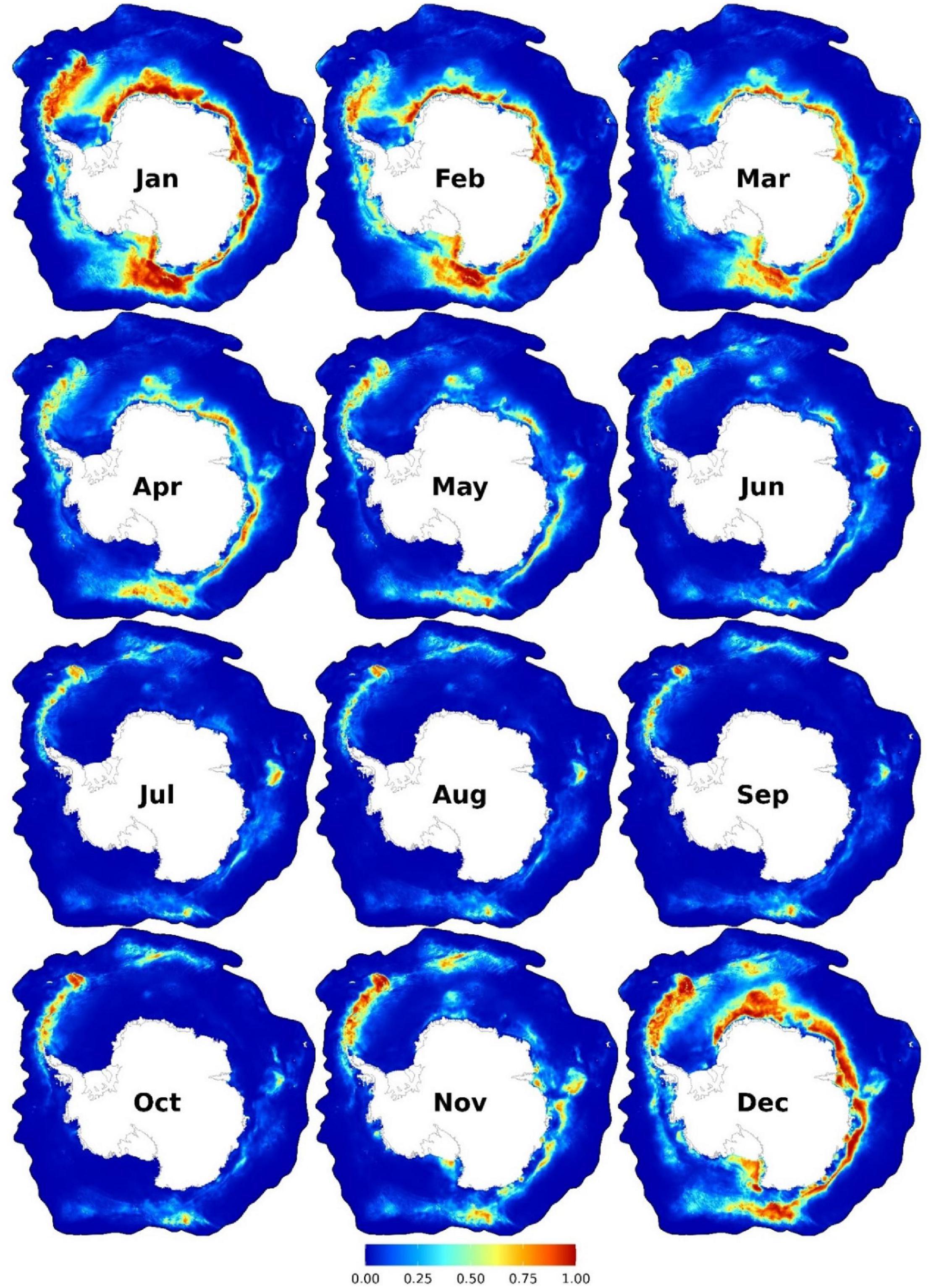
Figure 1. Monthly predicted habitat suitability for the Antarctic minke whales. Each map represents 90% quantile of daily habitat suitability from 2002 to 2019 in the respective month. Warmer colors represent higher habitat suitability. Other monthly and biweekly summary maps are shown in Supplementary Figures 4, 7.

FIGURE 2

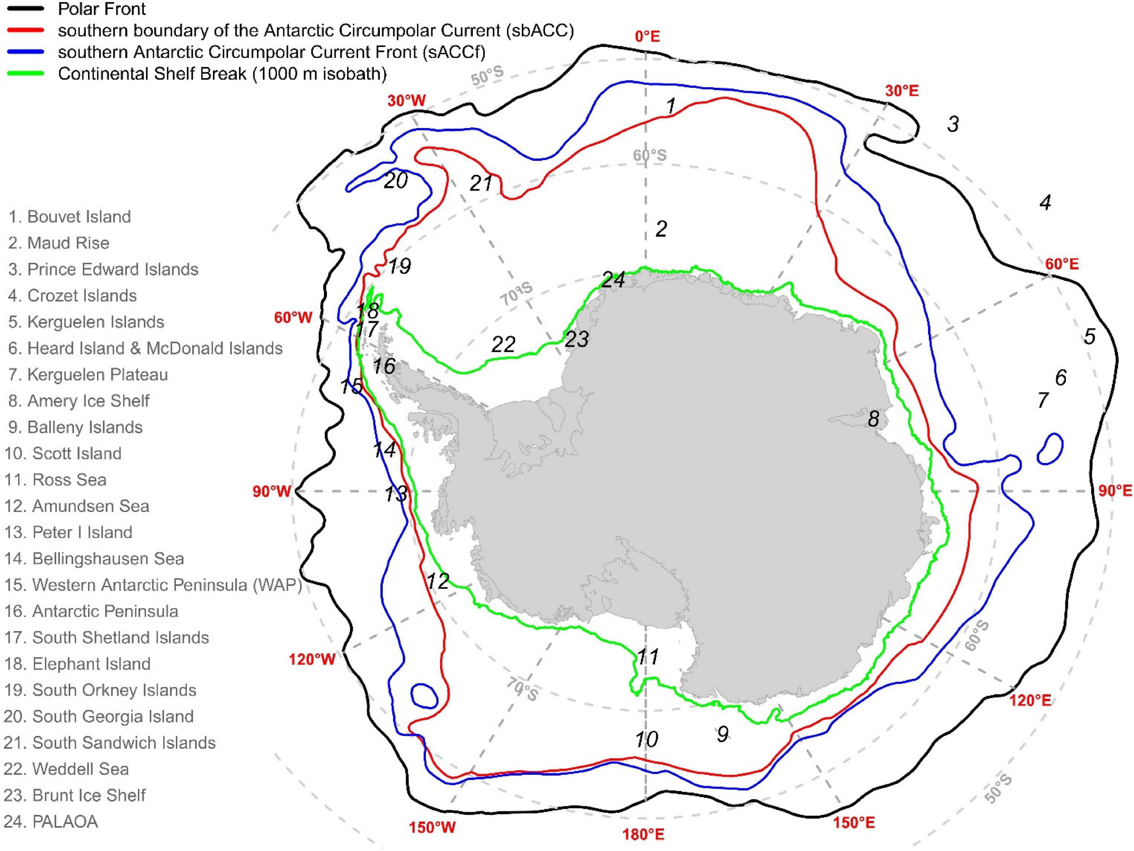
Figure 2. The geographical location of places mentioned in this manuscript. The location of the Polar Front, the southern boundary of the Antarctic Circumpolar Current (sbACC), and the southern Antarctic Circumpolar Current Front (sACCf) was plotted following Orsi et al. (1995).

FIGURE 3

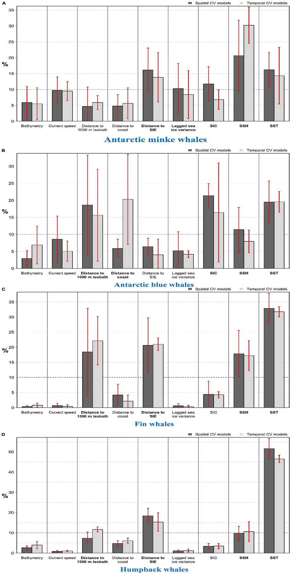
Figure 3. Permutation importance of predictors for the (A) Antarctic minke; (B) Antarctic blue; (C) Fin; (D) Humpback whale models. Permutation importance was calculated based on the drop in testing AUC after 150 permutations per predictor. Dark and light gray bars represent mean predictor importance for spatially and temporally cross-validated models, respectively. Red error bars show the standard deviation of the importance of the respective model. Predictors with >10% mean importance (horizontal dashed line) were considered important predictors and shown in bold names.

Antarctic Blue Whales

Suitable habitats were predicted from November to April, with peak suitability between December and February (Figure 4). Suitable areas were between the tip of the Antarctic Peninsula and the east of South Georgia and the South Sandwich Islands and coastal regions from the east of the Weddell Sea eastwards to the western coast of the Ross Sea. Further, other small patches of suitable habitats exist in East Antarctica (between the Kerguelen Plateau and the Kerguelen Islands) and the Bellingshausen and Amundsen Seas (Figure 4). The area east of the Antarctic Peninsula is predicted to be suitable year-round, albeit with relatively lower suitability in winter. Important predictors were SIC (<50%), SST (< 2°C, and > 5.5°C only near the coast or continental shelf break), 40–250 km from the coast, and < 200 km from the continental shelf break (Figure 3B and Supplementary Figures 17–18). High habitat suitability was also predicted at SSH ∼ -1.2 m, low speed (< 0.2 ms^–1), close to the SIE (especially on the open-water side of it), and moderate depths (1,500–4500 m) (Supplementary Figure 18).

FIGURE 4

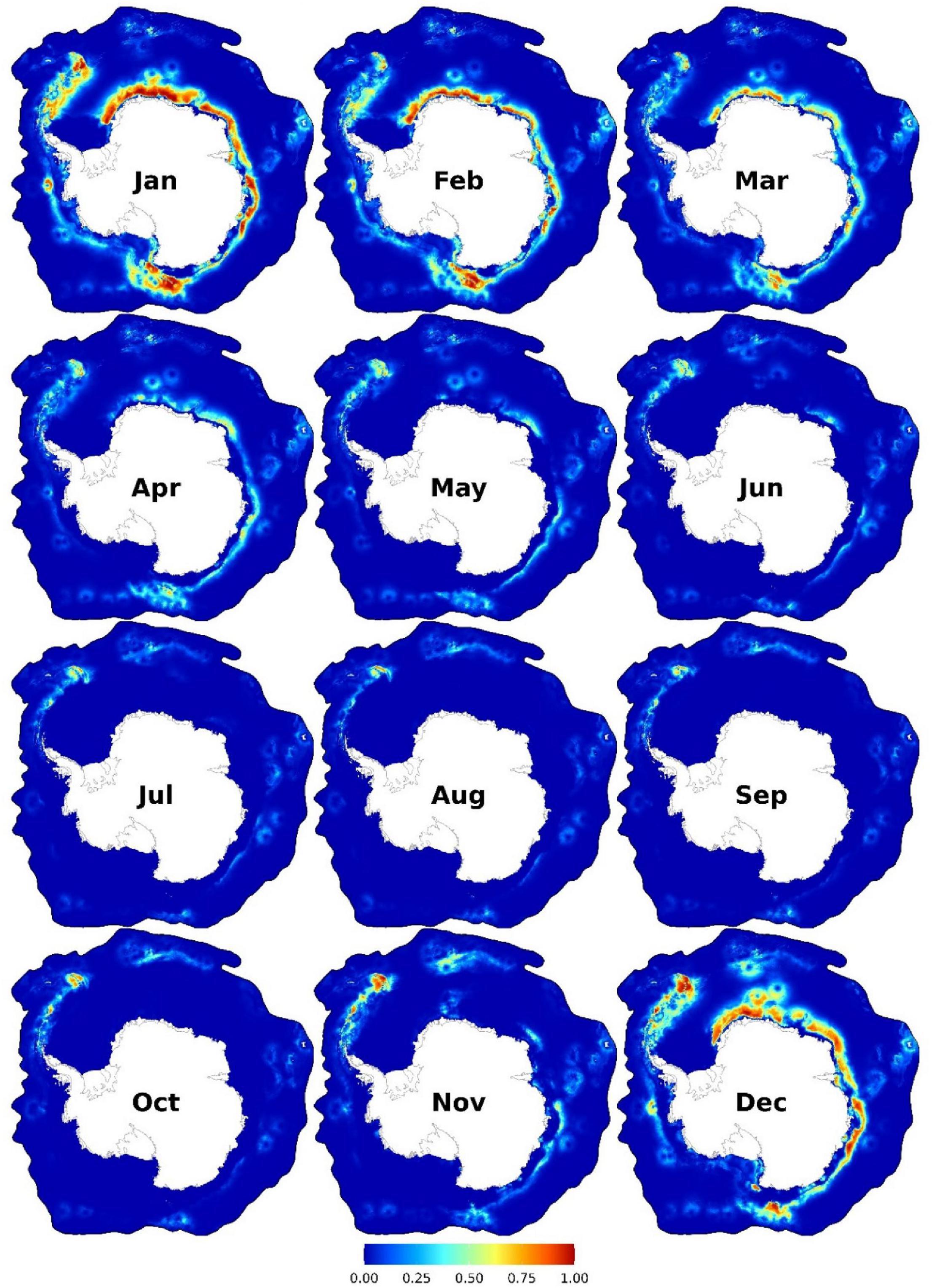
Figure 4. Monthly predicted habitat suitability for the Antarctic blue whales. Each map represents 90% quantile of daily habitat suitability from 2002 to 2019 in the respective month. Warmer colors represent higher mean habitat suitability. Other monthly and biweekly summary maps are shown in Supplementary Figures 12, 15.

Fin Whales

Highest habitat suitability is predicted from December to the end of May in the Amundsen Sea; the east of the Bellingshausen Sea toward South Georgia and the South Sandwich Islands; near Bouvet Islands; and offshore areas (∼200–300 km from Antarctica) from the Greenwich Meridian eastwards to the northwest of the Ross Sea (c.a. 160°W; Figure 5). From June to November, small patches of suitable habitats are predicted in relatively low latitudes. Important predictors are SST (particularly from -1 to 2.5°C), distance to the SIE (with two peaks predominately north of the SIE: up to ∼250 km and at ∼1,000–1,600 km north of it), distance to continental shelf break (< ∼450 km), and SSH (-1 to -1.5 m) (Figure 3C and Supplementary Figures 25–26). Two peaks of habitat suitability were predicted at shallow depths and ∼4,000 m (Supplementary Figure 26).

FIGURE 5

Figure 5. Monthly predicted habitat suitability for the fin whales. Each map represents 90% quantile of daily habitat suitability from 2002 to 2019 in the respective month. Warmer colors represent higher mean habitat suitability. Other monthly and biweekly summary maps are shown in Supplementary Figures 20, 23.

Humpback Whales

High habitat suitability is predicted from December to the end of April, particularly in the WAP (Figure 6). Other suitable habitats include near Bouvet Island and coastal area (albeit at c.a. 200 km from the Antarctic coast) from the Greenwich Meridian eastwards to ∼160°W. Important predictors are SST (mainly from -1 to 3°C, and up to 5°C only at low SSH or near the SIE), distance to the SIE (predominately in the open-water side of it, either close to it or at ∼1,000–1,500 km from it), distance to continental shelf break (< 450 km), and SSH (< -1.1 m) (Figure 3D and Supplementary Figures 33–34).

FIGURE 6

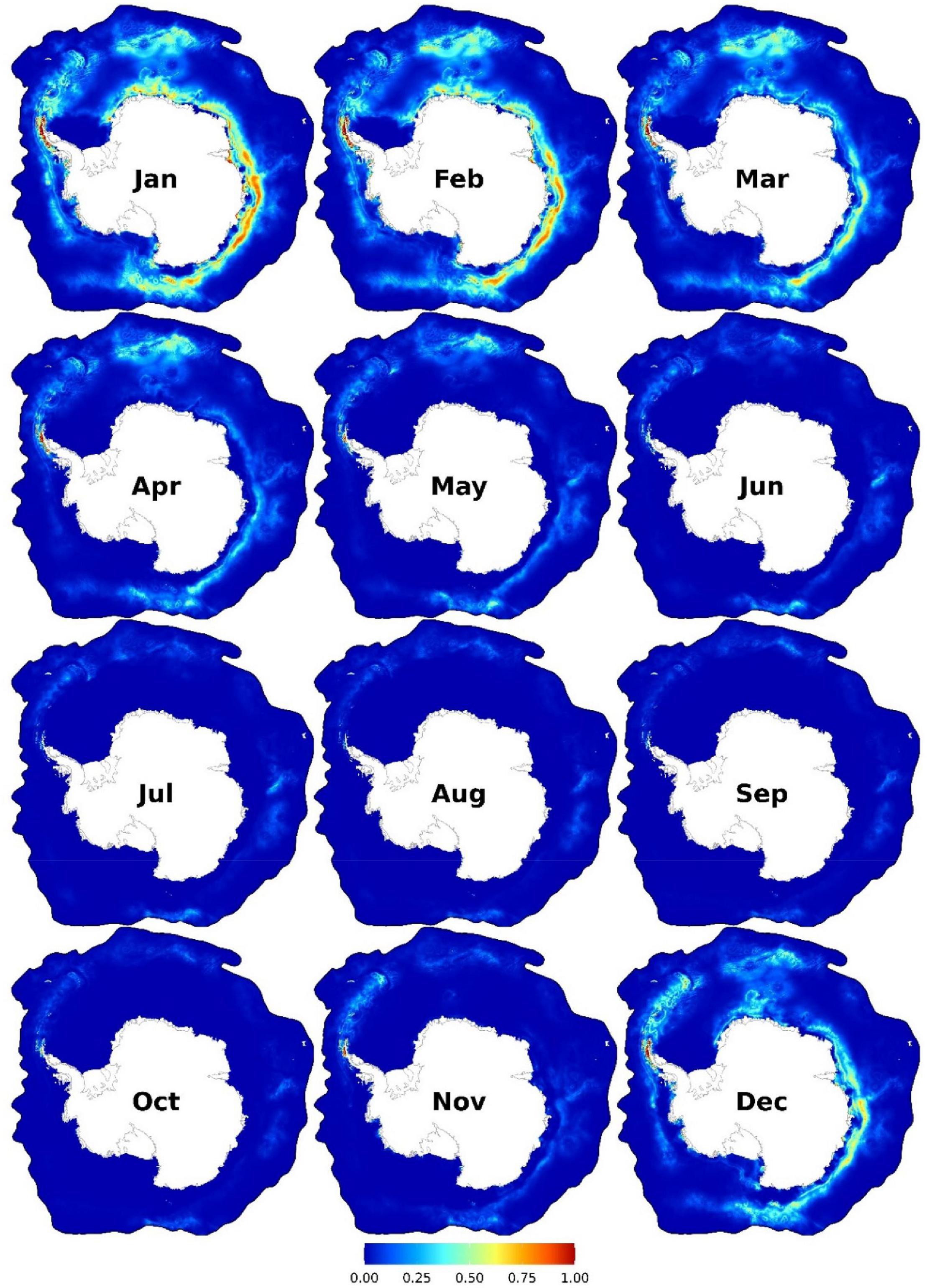
Figure 6. Monthly predicted habitat suitability for the humpback whales. Each map represents 90% quantile of daily habitat suitability from 2002 to 2019 in the respective month. Warmer colors represent higher mean habitat suitability. Other monthly and biweekly summary maps are shown in Supplementary Figures 28, 31.

Discussion

Spatiotemporal Habitat Suitability of Baleen Whales in the Southern Ocean

Antarctic Minke Whales

AMWs are reported to be present year-round in the SO and have a circumpolar distribution (Risch et al., 2019; Filun et al., 2020). The AMWs’ year-round presence is mainly supported by passive acoustic monitoring (PAM) data (Van Opzeeland, 2010; Dominello and Širović, 2016; Filun et al., 2020; Shabangu et al., 2020b). However, the majority of recent sightings used here (after 2002) were observed from December to May near the SIE (see Supplementary Figures 3, 9–10), with very limited occasional winter sightings (e.g., Van Franeker et al., 2008; Burkhardt, 2009a,b). Nevertheless, relatively older sightings support the winter presence of AMW in the SO (Taylor, 1957; Erickson, 1984; Plötz et al., 1991; Aguayo-Lobo, 1994; Ribic et al., 1999; Thiele and Gill, 1999).

Our models predict nearly year-round habitat suitability for AMWs along the WAP to South Georgia and the South Sandwich Islands and in East Antarctica, particularly from October to June (Figure 1). In this area, the SIE (particularly in summer) abuts with two ecologically important oceanographic features: the southern boundary of the Antarctic Circumpolar Current (sbACC) and the continental shelf break (see Figure 2). Together with the SIE, both features are important factors affecting the abundance of top predators (Tynan, 1998; Ribic et al., 2011), which supports the high ecological importance of this area (Friedlaender et al., 2021). AMWs feed predominantly on Antarctic krill (Euphausia superba; hereafter krill) (Beekmans et al., 2010; Williams et al., 2014), and the continental shelf break is known for high krill abundance throughout the SO (Siegel, 2005; Nicol, 2006; Ainley et al., 2012; Siegel and Watkins, 2016). Albeit our models did not identify distance to continental shelf break among the most important predictors, high habitat suitability was predicted closer to it (Figure 3 and Supplementary Figure 10), in concordance with results from previous studies (Ichii, 1990; Beekmans et al., 2010; Santora et al., 2010; Ainley et al., 2012; Herr et al., 2019; El-Gabbas et al., 2021a). Upwelling, high primary productivity, and krill peak distribution are generally found near, and particularly south of, the sbACC (Tynan, 1998; Nicol et al., 2000; Constable et al., 2003; Atkinson et al., 2008; Bost et al., 2009), which can explain the AMW near-year-round predicted habitat suitability at this hotspot area. Ainley et al. (2012) reported an AMW peak suitability near the sbACC, while Lee et al. (2017) found a strong association between satellite-tagged AMWs and the sbACC, with three tracked animals having remained south of it during the foraging season. Between December and April, other high suitability areas form a crest extending from the Weddell Sea (30°W) eastwards to the Ross Sea (160°W) and near the Balleny Islands (Figure 1). These coastal areas overlap with the location of the continental shelf break and the SIE during this period. Coastal areas from c.a. 30 to 170°E overlap with areas with the frequent AMW sightings in the Indo-Pacific sector of the SO during independent summer surveys (Matsuoka and Hakamada, 2020) and with the location of the sbACC (Figure 2).

Sea ice conditions and the position of the SIE have been reported as important factors affecting the habitat of AMWs (Kasamatsu et al., 2000a; Herr et al., 2019). Our models predict a negative relationship between AMW habitat suitability and SIC (Supplementary Figure 10), which was similarly reported by Herr et al. (2019) and El-Gabbas et al. (2021a). In contrast, Dominello and Širović (2016) and Filun et al. (2020) found a positive correlation between SIC and AMW acoustic presence in winter. This positive correlation may be caused by AMWs calling predominantly in winter, with much less calls during the foraging season, despite frequent sightings of AMWs during this period (Van Opzeeland, 2010; Risch et al., 2014; Shabangu et al., 2020b). A similar seasonal pattern of AMW calls was observed off Namibia (Thomisch et al., 2019) and Chile (Buchan et al., 2020), areas free of sea ice year-round, questioning a direct positive effect of SIC on AMW acoustic presence. Our models predict high suitability close to the SIE irrespective of SIC and generally low suitability farther away from it, which agrees with previous studies (Kasamatsu et al., 2000a; Thiele et al., 2000; Murase et al., 2002; e.g., Beekmans et al., 2010; Scheidat et al., 2011; Murase et al., 2013; Williams et al., 2014; Herr et al., 2019; Matsuoka and Hakamada, 2020; El-Gabbas et al., 2021a). High primary production and krill abundance are known to occur along and just south of the SIE (Brierley et al., 2002; Murase et al., 2002), supporting the foraging of many predators, AMWs in particular (Thiele et al., 2004; Friedlaender et al., 2006; Herr et al., 2019).

AMWs are well-adapted to exploit pack ice areas (Ainley et al., 2007; Lee et al., 2017). They were frequently observed within heavily sea ice-covered areas, associated with pancake and new ice near the marginal ice zone and use leads for breathing (Ribic et al., 1999; Ainley et al., 2007, 2012; Bombosch et al., 2014). Further, AMWs were observed creating holes in newly formed ice for breathing (Ainley et al., 2007, 2012; Tynan et al., 2009). The strong preference of AMWs to sea ice habitats can be considered as protection against predation by killer whales, which occurs mainly in open waters (Friedlaender et al., 2021). In addition to the frequent AMW sightings near the SIE, literature reported AMW sightings in pack ice areas. For example, Naito (1982): 167 km south of the SIE in the Lützow-Holm Bay by the end of December; Ensor (1989): ∼900 km south of the SIE north of Prydz Bay in October-November; Thiele and Gill (1999): 180–350 km south of the SIE in July off Dibble Iceberg Tongue; and Ribic et al. (1999) who reported that the majority (90%) of AMW observations occurring in the pack ice area of the southern Scotia Sea in winter. Available recent sightings (after 2002) show that only a few AMW observations were made far south of the SIE (> 400 km), mainly from icebreaker RV Polarstern expeditions along the Greenwich Meridian and in the center of the Weddell Sea (Burkhardt, 2009a,2013a; Williams et al., 2014).

Our models predict high habitat suitabilities at some locations far south from the SIE from November to February, particularly in coastal polynyas; e.g., off the Amery and Brunt ice shelves, and the Balleny Islands and in the Ross and Bellingshausen Seas (see Supplementary Figure 8 and animated video in El-Gabbas et al., 2021b). Coastal polynyas are likely hotspots in the pack ice, as they provide enhanced primary and secondary production, including krill, and open-water access for birds and mammals for breathing far within the pack ice (Gill and Thiele, 1997; Arrigo and Van Dijken, 2003; Van Opzeeland et al., 2013; Arrigo et al., 2015; Hunt et al., 2016; Labrousse et al., 2018). The observation of AMWs in polynyas and ice gaps was reported in other studies (Taylor, 1957; Naito, 1982; Ainley et al., 2006, 2007; Bester et al., 2017; Konishi et al., 2020; Shabangu et al., 2020b). The high habitat suitability in some polynyas and the sightings south of the SIE mentioned above support that AMWs are not restricted to near SIE but also exploit polynyas and heavily ice-covered areas within the pack ice and that the low number of sightings far south of the SIE or at high SIC values can be an artifact of sampling constraints.

AMWs are currently classified as “Near Threatened” by the International Union for Conservation of Nature (IUCN) (Cooke et al., 2018). Although AMW populations have undergone rapid increase during the twentieth-century (Tulloch et al., 2019), their strong dependence on sea ice as habitat and krill for food suggests that AMWs are further at high risk of climate change (Thiele et al., 2004; Lee et al., 2017; Herr et al., 2019; Risch et al., 2019; Konishi et al., 2020). AMW habitats are expected to narrow considerably during the upcoming decades (Ainley et al., 2012), with a predicted slow population growth rate over the next 100 years (Tulloch et al., 2019). Climate change is expected to affect the amount, quality, and interannual variability of sea ice, the location and length of the SIE, the abundance and distribution of krill, the prevalence of coastal polynyas, and shifting sbACC southwards (Ainley et al., 2007, 2012; Nicol et al., 2008; Beekmans et al., 2010; Friedlaender et al., 2011; Gutt et al., 2015; Atkinson et al., 2019). Therefore, understanding the niche preferences of the AMWs in the SO and its relationship to sea ice is essential for AMWs conservation under climate change.

Antarctic Blue Whales

Currently, ABWs are rarely sighted in the SO after being harvested to near extinction during commercial whaling, resulting in the extermination of 99% of the estimated pre-whaling population (Branch et al., 2007). ABW estimated abundance has depleted from 239,000 during pre-whaling to as few as 360 in 1973 (Branch et al., 2004), with the most recent circumpolar abundance estimate of c.a. 3,000 individuals (Branch, 2007; Cooke, 2018a). ABWs are the least observed species in our study, sparsely distributed in space, with most sightings observed in January/February (Supplementary Figure 11). They are currently classified as ‘Critically Endangered’ by IUCN (Cooke, 2018a), and their distribution is poorly understood at large spatial and temporal scales (Branch et al., 2007; Thomisch et al., 2016).

ABW suitable habitats are predicted mainly from November to April, peaking between December and February (Figure 4), overlapping in time with the majority of SO’s historical catch data (Risting, 1928; Horwood, 1986). Our models show a latitudinal shift in daily habitat suitability from (the low-to-moderately suitable) mid-latitudes in mid-October poleward to the most southern suitable areas near the Antarctic coast in mid-February, followed by a northward shift until low circumpolar suitability is predicted generally from late May to October (see El-Gabbas et al., 2021b for animated videos). Distance to coast was one of the important predictors, with high habitat suitability relatively close (40–250 km) to the coast (Figure 3B and Supplementary Figures 17–18). Shabangu et al. (2017) reported similar results using PAM data and highlighted that ABWs prefer highly productive areas closer to the Antarctic coast. Our models predicted high habitat suitability in coastal areas from the eastern margins of the Weddell Sea eastwards to the western coast of the Ross Sea (Figure 4). These areas overlap with historical catch data (Kellogg, 1929; Horwood, 1986; Branch et al., 2007), old sightings (before 2002) excluded from our analyses (Supplementary Figure 11E), and other recent independent visual and PAM data (Nishiwaki et al., 1997; Rankin et al., 2005; Gedamke and Robinson, 2010; Matsuoka and Hakamada, 2014; Miller et al., 2015; Mogoe et al., 2016, 2017, 2019; Isoda et al., 2017, 2020). In this area, the continental shelf break, summer SIE, and the sbACC (only from ∼ 45°E to 170°W) overlap, which can explain the high krill abundance (Tynan, 1998; Atkinson et al., 2017) and predicted habitat suitability (Cuzin-Roudy et al., 2014) in this area. The distance to the sbACC is an important predictor for ABW call presence in the SO (Shabangu et al., 2017). Our models identified distance to continental shelf break among the most important predictors, with predicted habitat suitability being the higher the closer to it (Figure 3B and Supplementary Figures 17, 18). In concordance, Miller B. S. et al. (2019) showed a high occurrence of ABW calls along the continental shelf break off East Antarctica (138°–152°E), while coastal area off Queen Maud Land was recently suggested as an ABW hotspot area, supported by visual sightings (Paarman et al., 2021) and PAM data (Shabangu et al., 2020a) as well as predictions from our models.

The migratory pattern of ABWs is complex and non-obligatory (Leroy et al., 2016; Thomisch et al., 2016; Torterotot et al., 2020). PAM data show evidence that at least some animals overwinter at high latitudes (Širović et al., 2009); e.g., off the Antarctic Peninsula (Širović et al., 2004, 2009; Dziak et al., 2015), East Antarctica (Širović et al., 2009; Gedamke and Robinson, 2010), the Weddell Sea (Thomisch et al., 2016), and off Maud Rise (Shabangu et al., 2020a). ABW calls in the SO show a seasonal pattern, with low acoustic detections in winter (Širović et al., 2004, 2009; Branch et al., 2007; Thomisch et al., 2016) and a more evident year-round presence at PAM stations at lower rather than higher latitudes (Širović et al., 2009). The ABW year-round presence at the SO’s high latitudes is not an exception: ABWs are acoustically detected year-round at mid-latitude locations in the sub-Antarctic and subtropical sections of the Indian Ocean (Samaran et al., 2010, 2013; Leroy et al., 2016, 2018; Torterotot et al., 2020) and off Namibia (Thomisch et al., 2019). The definite nature of ABWs migration (and probably other baleen whale species) is not yet clear and can include either partial or differential migration or a mixture of both (Thomisch, 2017). Our models identify near-year-round high habitat suitability in the east of the Antarctic Peninsula. While most historical catches were harvested between October and May (Risting, 1928; Harmer, 1931; Kemp and Bennett, 1932; Branch et al., 2007), year-round ABW catches were reported off South Georgia and South Shetland Islands (Hinton, 1915; Risting, 1928; Kellogg, 1929; Harmer, 1931; Hjort et al., 1932). Although this area was a main ABW commercial whaling site, the extensive exploitation caused ABWs to be currently rare there (Moore et al., 1999; Clapham et al., 2008; Leaper and Miller, 2011). Nevertheless, recent work suggests the start of ABW recovery from this area (Calderan et al., 2020), and our models further support the importance of this area as near-year-round habitat for ABWs. Other predicted near-year-round suitable habitats include the east of Bouvet Island and off the Kerguelen Plateau, although with generally low suitability in winter. PAM data from the Southern Indian Ocean (e.g., Leroy et al., 2016) further support the importance of the area north of the Kerguelen Plateau as year-round suitable habitat for ABWs. Our models predict high habitat suitability at low SIC values and close to the SIE (Supplementary Figures 17, 18). Daily habitat suitability maps show that ABW suitable habitats are generally limited to the vicinity of the SIE and rarely south of it (see El-Gabbas et al., 2021b for animated videos). Information derived from PAM (Shabangu et al., 2017) and visual sightings (Kasamatsu et al., 1988, 2000b; Širović et al., 2009) suggests that following the twentieth-century heavy exploitation, the distribution of ABWs is currently confined to along the SIE in summer where krill is more abundant, whereas historical catches extended farther north of the pack ice (Branch et al., 2007; Leaper and Miller, 2011). Acoustic data support the general avoidance of ABWs of heavily sea ice-covered areas (Širović et al., 2004), with an estimated negative correlation between SIC and ABW calls (Širović et al., 2004; Thomisch et al., 2016). Thomisch et al. (2016) found that the majority of calls were detected during low or moderate sea ice conditions, although some calls were also detected at high SIC (>90%) in winter, suggesting that ABWs show some tolerance to high sea ice conditions (i.e., is not restricted to ice-free areas) (Double et al., 2015; Thomisch et al., 2016). This is supported by some historical ABW catches in drifting ice in the pack ice area (Slijper, 1962; Horwood, 1986). South of the SIE, our models predicted high suitability in coastal polynyas near the Amery and Brunt ice shelves and in the Ross Sea in December and January (Supplementary Figure 16). This supports the critical role of coastal (particularly recurrent) polynyas as habitat, particularly during austral summer, for many baleen whale species, including ABWs, providing animals with food and access to open water for breathing (Tynan et al., 2009; Thomisch et al., 2016). Nevertheless, there is no visual evidence available to us for the actual occupation of polynyas by the large ABWs.

ABWs are predicted to undergo further substantial abundance reduction by the end of the twenty-first century (Tulloch et al., 2019) due to, e.g., krill biomass reduction resulting from overfishing and potential loss of sea ice in response to climate change (Wiedenmann et al., 2011). ABW habitats are highly vulnerable to future climate change (Shabangu et al., 2017), which could impede the recovery of ABWs and a higher conservation risk. This urges the need for dedicated surveys and tagging studies to monitor the ABW population (Tulloch et al., 2019), which can be used in combination with year-round PAM data to improve our understanding of ABW ecology and assess population trends and their future threats (Thomisch et al., 2016; Calderan et al., 2020).

Fin Whales

FWs were the most frequently caught whale species in the SO during the commercial whaling era (Clapham and Baker, 2002; Leaper and Miller, 2011; Santora et al., 2014). Globally, FWs are currently classified as “Vulnerable” by IUCN Red List (Cooke, 2018b). However, little information is known about their abundance and distribution in the SO (Branch and Butterworth, 2001; Herr et al., 2016). Recent years show signs of slow population recovery, particularly in the WAP area (Joiris and Dochy, 2013; Santora et al., 2014; Reyes Reyes et al., 2015; Burkhardt et al., 2021). Nevertheless, FWs are projected to undergo further population decline by 2100 due to climate change (Tulloch et al., 2019), which urges the need for identifying and protecting their key habitats and better management of anthropogenic activities in the SO to ensure FWs’ unhindered recovery (Santora et al., 2014; Burkhardt et al., 2021).

Our models predict high habitat suitability mainly from December to May (peaking in February), with low-to-moderate suitability during autumn and winter only at lower latitudes (Figure 5). This largely agrees with the known information on FW temporal distribution in the SO, as derived from visual sightings (Kasamatsu et al., 1996) and historical catches (Hjort et al., 1932; Kemp and Bennett, 1932; Ohno and Fujino, 1950). However, recent PAM data shows that FW acoustic presence (as represented by 20-Hz pulses) starts and ceases significantly later than their reported visual presence near the Elephant Island area (Burkhardt et al., 2021). FW 20-Hz pulses show a strong seasonal pattern, occurring mainly between mid-February and July, with a peak detection in May, and only occasional pulses in the remainder of the year (Širović et al., 2004, 2007, 2009; Baumann-Pickering et al., 2015; Shabangu et al., 2020a; Burkhardt et al., 2021; Miller B. S. et al., 2021). Combined information derived from our models and PAM data suggests FW presence in the SO from at least from December to August (Burkhardt et al., 2021).

High suitability areas (Figure 5) coincide with independent datasets and known FW hotspot areas; e.g., the Antarctic Peninsula area (Santora et al., 2014; Herr et al., 2016); near Elephant Island (Thiele et al., 2004; Burkhardt and Lanfredi, 2012; Joiris and Dochy, 2013; Viquerat and Herr, 2017; Bassoi et al., 2020; Burkhardt et al., 2021); around South Orkneys (Viquerat and Herr, 2017); the Scotia Sea (Orgeira et al., 2017); the Maud Rise (Shabangu et al., 2020a); East Antarctica (Nishiwaki et al., 1997; Matsuoka and Hakamada, 2014; Isoda et al., 2017; Mogoe et al., 2017, 2019); and near Bouvet Island (Ensor et al., 2007). Suitable habitats were predicted between the Southern Antarctic Circumpolar Current Front (sACCf) and south of the sbACC (Figure 2), particularly along the WAP eastwards; near Bouvet Island; north of the Balleny Islands; and in East Antarctica. Both oceanographic features are important productivity areas which support high prey availability. Therefore, not surprisingly several studies suggested an association between FW concentrations along and just south of the sbACC (Tynan, 1998; Santora and Veit, 2013; Viquerat and Herr, 2017; Matsuoka and Hakamada, 2020); while Širović et al. (2006) and Bassoi et al. (2020) reported a higher concentration of FWs near the sACCf. Further, Širović et al. (2009) and Santora et al. (2014) found high FW call detections and visual sightings, respectively, between the sbACC and the sACCf.

The relationship between sea ice conditions and FW habitat and behavior in the SO may have not been fully understood yet. Our models show a negative relationship between sea ice and FW habitat suitability: high suitability at low SIC and>100–200 km north of the SIE. In contrast to other study species, only moderate suitability is predicted near the SIE, with very low values south of it. This conforms with the current knowledge that FWs are pelagic species, negatively correlated with SIC, and absent from heavily sea ice-covered areas (Kasamatsu et al., 1996, 2000b; Širović et al., 2004, 2006; Cooke, 2018b; El-Gabbas et al., 2021a). In the available dataset, the only FW sightings south of the SIE occurred SSW of Elephant Island (April 2012): 35 km south of the SIE at high SIC values (81–93%) (Burkhardt, 2013b). In a recent study, Burkhardt et al. (2021) showed that FW acoustic occurrence off Elephant Island diminishes clearly before the start of sea ice formation (also shown in Širović et al., 2004), which suggests that FW acoustic presence is not directly related to the growth of sea ice (i.e., sea ice formation does not lead to animals moving northwards toward the north of the SIE), but other factors such as depletion of prey abundance (Burkhardt et al., 2021). Furthermore, our models also predict moderate habitat suitability in small coastal polynyas in the Ross Sea, near the Amery ice shelf, and at small coastal areas in the Weddell and the Bellingshausen Seas in January (Supplementary Figure 24). However, it is unclear if these coastal polynyas represent habitats that FWs actually occupy as these areas are bordered by heavily ice-covered waters (effectively inaccessible FW) and are further south than FWs to date are known to migrate.

Humpback Whales

Our models predict high HW habitat suitability in the WAP area from mid-October to May, and to a lesser extent, in June (Figure 6). The WAP is a well-known HW hotspot area in summer and autumn (Stone and Hamner, 1988; Thiele et al., 2004; Nowacek et al., 2011; Johnston et al., 2012; Friedlaender et al., 2013; Bester et al., 2017; Reisinger et al., 2021). Krill is the primary food source of HWs, and the distribution and movement of HWs are highly associated with the distribution and abundance of krill (Murase et al., 2002; Nowacek et al., 2011; Curtice et al., 2015; Weinstein et al., 2017; Friedlaender et al., 2021). The WAP area is known to support large populations of krill and their predators (Friedlaender et al., 2006, 2013, 2021; Nowacek et al., 2011; Atkinson et al., 2017) because of the nutrient-rich and phytoplankton-laden water near the surface advected along the WAP by the Antarctic Circumpolar Current and nutrient-rich Circumpolar Deep Water being upwelled in the cross-shelf deep water canyons (Curtice et al., 2015) along the WAP’s northern shelf break.

Further moderate-to-high suitable habitats are predicted from December to mid-March near Bouvet Island and a band c.a. 200 km from the Antarctic coast from the Greenwich Meridian eastwards to the Balleny Islands (Figure 6). These areas of high habitat suitability overlap well with locations of independent data; including historical catch data (Omura, 1973; Matsuoka et al., 2006a), PAM data (150–180°E, Miller et al., 2017), and visual sightings (Matsuoka et al., 2006a,b; Hakamada and Matsuoka, 2013). These coastal areas (particularly 50–170°E) concur with the sbACC (including the area just south of it), an important oceanographic feature for HW distribution (Tynan, 1998; Matsuoka et al., 2003, 2006a). Furthermore, this area is located near the SIE in summer, which is characterized by high productivity and krill abundance (Nicol, 2006). The high HW suitability off Bouvet Island concurs with summer PAM data (Miller et al., 2017) and the frequent detections from this area using visual and telemetry data (Engel and Martin, 2009; Rosenbaum et al., 2014). This area shows large aggregations of krill (Siegel, 2012; Siegel and Watkins, 2016) and represents an important feeding ground for the West African HWs (breeding stocks B) (Rosenbaum et al., 2014; Seakamela et al., 2015). This high productivity area (Perissinotto et al., 1992) overlaps with the location of the sbACC and the sACCf (Figure 2). By contrast, low habitat suitability was generally predicted from May to November.

Our models predict low habitat suitability in the Weddell and Ross Seas. The HW absence from the Ross Sea, particularly south of 72.5°S, is well recognized although the extensive sampling from this area (Matsuoka et al., 2006b; Ainley, 2009; Branch, 2011; Hakamada and Matsuoka, 2013). HW observations from the Ross Sea area are confined to the north of the entrance of the Ross Sea; e.g., along the shelf break off Adélie Land coast (Ainley, 2009; Branch, 2011). The absence of HWs from the southern parts of the Ross Sea may be due to their high exploitations during the commercial whaling era or that the area has never been inhabited by HWs (Branch, 2011). This can be due to 1) HWs’ preference to avoid areas with high sea ice concentrations unsuitable with their body shape and long pectoral fins; or 2) HW’s possible aversion to ice krill (Euphausia crystallorophias), dominating the area south of 73°S in the Ross Sea (Sala et al., 2002; Branch, 2011). Dalla Rosa et al. (2008) reported a low HW density in the Weddell Sea. No sightings were available from the Weddell Sea, except along the Greenwich Meridian and northwest of the Weddell Sea near the Antarctic Peninsula (but see information from PAM data below). According to historical catch and recent visual and satellite-tracking information, the Kerguelen Plateau area is an important feeding area for the Australian HW population in summer due to its high productivity (Mackintosh, 1942; Omura, 1973; Tynan, 1997; Matsuoka et al., 2006b; Bestley et al., 2019). Nevertheless, our models predict low habitat suitability near the Kerguelen Plateau northwards, with suitable habitat only at the south of it close to the location of the sbACC and the SIE, in concordance with Tynan (1997).

The temporal distribution of suitable habitats (Figure 6) agrees, all in all, with the current state of knowledge by means of visual observations (Kasamatsu et al., 1996) and catch data (Matthews, 1937; Mackintosh, 1942). Historical catch data off South Georgia and the South Shetland Islands peaked in January, with another smaller peak in May (Matthews, 1937). Matthews (1937) related these two peaks to the arrival and departure of HWs from the SO. Nevertheless, historical catch data also provided evidence that not all HWs leave the SO in winter: many HWs were caught in the 1910s off South Georgia in May-June (Risting, 1928; Matthews, 1937). Since the cessation of commercial whaling, very limited HW winter sightings were reported from the SO: e.g., two individuals were observed in coastal fjords in the WAP in early August 2002 (Thiele et al., 2004).

Recent PAM data showed a nearly year-round HW acoustic presence in the Weddell Sea and the WAP (Mckay et al., 2004; Van Opzeeland et al., 2013; Schall et al., 2020). Interestingly, low (January-February) or no (December) HW acoustic presence was detected off Elephant Island during summer (Schall et al., 2020), despite the visual observation and high habitat suitability predicted during the same period. HW’s near-year-round acoustic presence and incidental winter sightings support that part of the HW population remains at high latitudes during winter (Thiele et al., 2004; Van Opzeeland et al., 2013; Schall et al., 2020). Brown et al. (1995) showed evidence that some HW females overwinter in the SO feeding grounds. This is probably an advantage for some adult females to avoid the high energetic cost of migration and reproduction in some years (Brown et al., 1995; Van Opzeeland et al., 2013; Druskat et al., 2019; Schall et al., 2020).

Our models show that suitable habitats for HWs are located along and north of the SIE, following its retreat during austral spring/summer (see El-Gabbas et al., 2021b for animated videos). Likewise, previous studies indicate that HWs prefer ice-free areas (Dalla Rosa et al., 2008; Bombosch et al., 2014; Schall et al., 2020; El-Gabbas et al., 2021a) and are highly concentrated near the SIE and following it as it retreats (Thiele et al., 2004; Friedlaender et al., 2011; Bombosch et al., 2014; Riekkola et al., 2019; El-Gabbas et al., 2021a; Reisinger et al., 2021). The abundance of krill is highly related to the near or just south of the SIE (Daly and Macaulay, 1988; Brierley et al., 2002), which might be an explanation why HWs were often seen close to it. Our models predict a negative (albeit weak) relationship between HW habitat suitability and SIC (Supplementary Figure 34; see also El-Gabbas et al., 2021a). This agrees with the results of Schall et al. (2020, 2021), who found a weak correlation between SIC and HW acoustic presence in the Weddell Sea. Nevertheless, acoustic findings contradict the commonly recognized notion of HWs avoiding ice-covered areas: HWs were acoustically present nearly year-round, including high SIC values (> 90%) in winter, at the PALAOA station (on the Ekström Ice Shelf) (Van Opzeeland et al., 2013) and other PAM stations from the Weddell Sea (Schall et al., 2020). However, daily predictions from our models showed low predicted habitat suitability near the PALAOA station on days with HW acoustic presence from February to April. Although daily prediction maps show that HWs follow the SIE retreat, high habitat suitability is also predicted in small coastal polynyas in January and February (Supplementary Figure 32). Polynyas may provide HWs with access to open areas for breathing and enhanced productivity in winter (Van Opzeeland et al., 2013; Saenz et al., 2020; Schall et al., 2020). Nevertheless, and in contrast to AMWs, we are unaware of reported HW visual observations from SO polynyas, and the presence of HWs in coastal polynyas may require further investigations.

HWs are globally classified by the IUCN as “Least Concern” (Cooke, 2018c). However, HWs are predicted to be heavily impacted by future climate change (Meynecke et al., 2020): reaching full population recovery by 2050 then being reduced to half of their population by 2100 (Tulloch et al., 2019). In a recent study, Schall et al. (2021) showed a persistent HW acoustic presence in the Weddell Sea from 2011 to 2018, except during El Niño years 2015 and 2016, during which HWs were acoustically almost absent. Future climate change is predicted to increase the frequency of El Niño events (Cai et al., 2014), which might affect the spatiotemporal distribution and recovery of HWs in the SO (Schall et al., 2021). We compared HW biweekly and monthly habitat suitability from 2011 to 2018 and did not find a notable difference during the El Niño years. Furthermore, available sightings show consistent HW presence in the WAP during the summer from 2014 to 2016, indicating HW’s physical presence in the area also during El Niño years. The impact of El Niño on the SO’s ecosystem seems to be complex and mediated through reduced productivity and changes in sea-ice dynamics and krill abundance and recruitment (Quetin and Ross, 2003; Murphy et al., 2007; Loeb and Santora, 2015; Meynecke and Meager, 2016; Schall et al., 2021). This suggests that El Niño events can affect HW’s acoustic behavior and individual fitness, but not necessarily its physical presence or habitat suitability in the SO. The unnoticeable change in habitat suitability during El Niño years can be due to factors or processes not pronounced in the environmental data used in our model, e.g., changes in krill abundance. The effect of El Niño events on the SO’s ecosystem and particularly HW populations at high latitudes require further investigation.

Latitudinal Segregation in Species’ Suitable Habitats

From December to April, models predict overlap between suitable habitats of the four baleen whale species beyond c.a. 100–200 km from the Antarctic coast between 10°W eastwards to Scott Island (170°E) and at sparse locations from the WAP eastwards to South Georgia and the South Sandwich Islands, with more evident overlap from January to March (see Figure 7 and Supplementary Figure 36). The areas between 50°E and 170°E and at the WAP eastwards intersect with the area between the sbACC and the sACCf (Figure 2) and intersects with the location of the SIE during this period, which might explain the importance of these high productivity areas as key summer habitats for baleen whales. The area from the WAP toward South Georgia and the South Sandwich Islands is a well-recognized feeding habitat for the four species, supported by historical catch data and recent surveys (Kemp and Bennett, 1932; Richardson et al., 2012; Herr et al., 2016; Kennedy et al., 2020; Friedlaender et al., 2021).

FIGURE 7

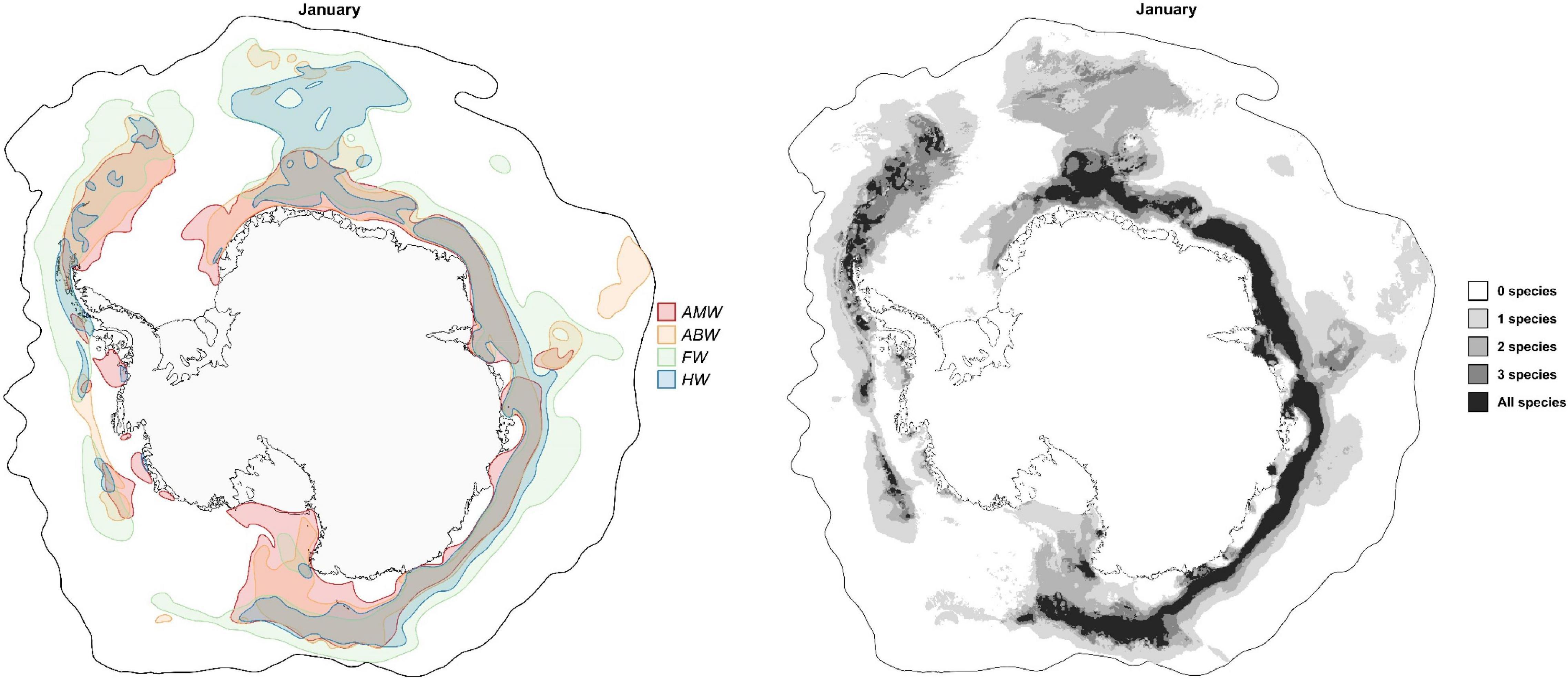
Figure 7. Overlap of predicted suitable habitats of baleen whales in the SO. The map to the left shows the overlap between smoothed suitable habitats in January. Colors represent possible combinations (AMW, Antarctic minke whales; ABW, Antarctic blue whales; FW, Fin whales; HW, Humpback whales). The map to the right shows the number of overlapping species (without smoothing) in January. Maps for monthly overlap are shown in Supplementary Figures 36, 37. Species-specific monthly suitable habitats are shown in Supplementary Figures 5, 13, 21, and 29, while the pairwise overlap between species’ suitable habitats is shown in Supplementary Figure 38.

To avoid competition between sympatric whale species over limited resources, species may use different ecological niches (e.g., feeding on different prey species) or partition the available resources (Friedlaender et al., 2009; Herr et al., 2016). Intraspecific morphological differences (e.g., the size and shape of the animal body and baleen plates) help baleen whales differ in their feeding behavior and the selection of prey type and size (Laws, 1977a). The study species show (not entirely) size-dependency predation of krill: HWs aggregate over small juvenile krill, AMWs over krill of intermediate size, ABWs over first-year krill, and FWs over large mature krill (Laws, 1977b; Santora et al., 2010; Miller E. J. et al., 2019), probably in relation to differences in their filter-feeding apparatus (Bassoi et al., 2020). Further, species show vertical resource partitioning, feeding separately on krill at different depths irrespective of the krill patch density: e.g., HWs in the top portion of the water column and AMWs at greater depths (Friedlaender et al., 2009).

To the north and south of these core areas that are predicted suitable for the four species together, models show latitudinal segregation in suitable habitats (Figure 7 and Supplementary Figure 36). Between December and May, areas closer to the Antarctic coast are primarily predicted suitable for AMWs but also overlapping sporadically with ABWs and HWs. AMWs are predicted to not overlap with other species in the southern Ross Sea, between Balleny and Scott Islands, and at sparse locations in the southern Amundsen and Bellingshausen Seas and in the east and center of the Weddell Sea. This strongly agrees with the pagophilic nature of AMWs, occupying pack ice areas (Ainley et al., 2012) for their high krill abundance, reducing competition with other mesopredators, and avoiding predation by killer whales in open waters (Laws, 1977a; Friedlaender et al., 2021).

FW and HW suitable habitats overlap at a small strip just north of the core area of the four species. At moderate-to-low latitudes, FWs are generally suitable in areas unsuitable for other study species. This is except for the area off Bouvet Island, which is predicted to be also suitable for HWs and sporadically for ABWs. FWs prefer open water areas and is rarely seen in the pack ice (Harmer, 1931; Hjort et al., 1932; Cooke, 2018b), with the majority of the population thought to occur north of 60°S (Laws, 1977b; Kasamatsu et al., 1996; Matsuoka and Hakamada, 2020). ABWs are predicted to not overlap with other species at an area between the north of the Kerguelen Islands to the south of Kerguelen Plateau (c.a. 70°E) and two small patches at moderate latitudes c.a. 62°S 150°W and in the Bellingshausen Sea (c.a. 68°S 100°W). This may indicate local spatial differences in prey composition, but we do not have sufficient data to examine this.

Dynamic Species Distribution Models in the Southern Ocean

Sighting Data Paucity and Spatiotemporal Biases

Using visual sightings, this study employed dynamic SDMs to predict the daily habitat suitability of four baleen whale species in the SO. Although these daily prediction maps have promising importance in conservation applications, the paucity and characteristics of available data might have affected the robustness of the model results. Recent baleen whale sightings from the SO are limited in space and time (Supplementary Figure 1; El-Gabbas et al., 2021a). Regular shipboard surveys are hindered by the SO’s remoteness and seasonal ice cover, implicating high costs and logistic efforts (Scheidat et al., 2011). In this study, we excluded sightings before June 2002 to maintain spatiotemporal matching between sightings and daily environmental predictors. Similarly, although historical catch data represents valuable information on the pre-whaling spatiotemporal distribution of the species, we cannot use these data in dynamic models. The species-environment relationship may have changed after the species’ extensive extirpation and changes in the physical environment during the last century, although evidence for this is yet unclear. Discarding older sightings resulted in a smaller sample size (see Supplementary Figures 3A,E, for example). The effect of discarding these data on the reliability of our model outputs depends on the amount of unique environmental combinations in these data not represented in recent sightings. Further, some important predictors were either incomplete at a large spatial scale, e.g. chlorophyll-a data from the SO is highly patchy outside of summer months, or not available at the appropriate spatiotemporal resolution, e.g., primary productivity and krill abundance (Herr et al., 2016; El-Gabbas et al., 2021a), disallowing using them in the current models.

Sighting data from the SO shows inevitable spatiotemporal biases (Supplementary Figure 1), which are expected further to lead to environmental bias. These biases need to be accounted for carefully during model calibration (Phillips et al., 2009; Merow et al., 2013; El-Gabbas and Dormann, 2018). We considered spatial sampling bias correction by using the estimated seasonal research effort to sample similarly biased daily background information (Supplementary Appendix 1 in the Supporting Information), a method commonly implemented to correct for spatial sampling bias (Phillips and Dudík, 2008; Merow et al., 2013). This assumes that the estimated research efforts correctly reflect the (typically unknown) spatial bias pattern in baleen whales sampling (Merow et al., 2013). However, this may not be a valid assumption; for example, if the used ship tracks dataset underrepresents the actual pattern of baleen whales’ research efforts or if it reflects unrelated activities (e.g., physical oceanography and geological studies). It is challenging to effectively correct for spatial sampling bias in dynamic SDMs in the SO, as the pattern of spatial sampling bias varies through time due to the waxing and waning of sea ice. Some sampling bias correction methods may not be applicable in dynamic models; for example, spatial filtering (rarefaction) (Aiello-Lammens et al., 2015) is commonly used in static SDMs to reduce the clumpiness of the data (e.g., El-Gabbas et al., 2021a). However, in dynamic SDMs, the frequent baleen whale sampling in easily accessed sites, e.g., the WAP, does not necessarily represent identical environmental combinations as the sampling at these sites was performed across many years. Therefore, discarding spatially clumped observations can result in excluding important environmental combinations.

Another related issue is that sightings show clear temporal bias toward the less harsh environmental conditions in austral summer months, particularly from mid-December to the end of February (Supplementary Figure 1). Seasonal sea ice prohibits efficient sampling from the south of the SIE and during the autumn/winter months (Bombosch et al., 2014; El-Gabbas et al., 2021a), restricting sampling efforts in the pack ice area to very few icebreaker-born surveys (e.g., Scheidat et al., 2011; Herr et al., 2019). Relatively recent winter sightings (after 2002) are very limited, with many of the older sightings observed in winter or south of the SIE being excluded from current models due to the lack of concurrent environmental data. Although the recognition that temporal sampling bias can result in environmental bias that may affect the model reliability, limited studies have investigated methods for correcting for the effect of temporal sampling bias (Ingenloff et al., 2020). It is challenging to correct for temporal sampling bias in the current data, as the problem is not the imbalanced sightings across time (e.g., higher sampling in summer than in winter), but the almost lack of sampling efforts from mid-March to mid-December (Supplementary Figure 1), particularly from high latitudes.

In the current models, we did not incorporate explicit information on the date or season of observation; i.e., the ability of the models to predict at a given combination of date and location is only ruled by the (n-dimensional) environmental similarity at this combination and environmental conditions at sightings. Therefore, data paucity and environmental biases in recent sightings might have affected the models’ ability to predict during autumn/winter months or south of the SIE. Nevertheless, our models were able to predict near-year-round habitat suitability at some locations and coastal polynyas south of the SIE, particularly in summer. It is important, however, to note that information on the location of daily polynyas was not explicitly incorporated into the models: as polynyas were assigned a positive distance to the SIE, the models do not differentiate between positive values at polynyas and positive values at cells just outside of the SIE. In future models, daily polynyas can be explicitly included in the model as a binary predictor (i.e., polynya/not-polynya). In order to be able to predict the winter distribution of baleen whales in the SO with high accuracy, obtaining more data beyond the summer months and from the south of the SIE is necessary. In such a case, the spatiotemporal (∼ environmental) bias can be considered in future models by environmentally filtering species data, discarding redundant information with similar environmental conditions (Varela et al., 2014).

Integrating Visual Sightings and Passive Acoustic Monitoring Data in Dynamic Species Distribution Models

As we emphasized above, gaps and spatiotemporal biases in sighting data highlight the need for more data, covering environmental combinations not presented in currently available data, particularly in austral winter and south of the SIE (El-Gabbas et al., 2021a). However, obtaining sufficient sightings across the vast SO at a large spatial scale and fine temporal resolution is hard, if possible. PAM data is very promising to complement our limited knowledge on the year-round spatiotemporal distribution of baleen whales derived from sighting data (Van Opzeeland et al., 2013) as PAM is unaffected by poor weather conditions, operates both day and night autonomously and omnidirectionally over extended periods. Additionally, it is capable of detecting species below the water surface, while not requiring the presence of researchers in the study area (Mellinger et al., 2007; Leroy et al., 2016; Frasier et al., 2021). PAM is particularly useful in the SO for detecting rarely visually sighted species like ABWs, which are regularly detected in acoustic recordings (Gedamke and Robinson, 2010). Further, PAM can detect species presence in areas that are difficult to access, e.g., when they are permanently or seasonally ice-covered and typically do not exhibit temporal biases compared to sightings data.

However, PAM data requires careful pre-processing before being used in SDMs. One difficulty in using acoustic data for dynamic SDMs is the potential spatial mismatch between the acoustic recorder location and the actual calling position of the animals, which results from the fact that marine mammal sounds, especially low-frequency baleen whale vocalizations (e.g., ABWs), can propagate over long distances (Širović et al., 2007; Širović and Hildebrand, 2011). Also, PAM data is frequently collected over extended periods from fixed sensors at a few locations, which may not well represent environmental conditions in the entire area of interest. The degree to which environmental conditions (and their combinations) at a few fixed locations (e.g., Van Opzeeland et al., 2014) representing the environmental conditions at the vast SO needs to be assessed before using these data to predict the circumantarctic habitat suitability of the species to avoid environmental extrapolation. Further, the less understood behavioral context of sound production for some baleen whale species represents a hurdle of the efficient use of PAM data (Mellinger et al., 2007). PAM occurrence only represents vociferous animals: animals can be physically present near the detector but not-calling because of behavioral reasons (Verfuss et al., 2018). Therefore, SDM outputs using PAM data can be sensitive to the acoustic behavior of the vocalizing animals. In conditions at which species’ acoustic behavior covary with values of an important environmental predictor, it can be challenging to correctly estimate the relationship between the species habitat suitability and this predictor. For example, the more frequent AMW calls at high latitudes during austral winter than in summer may suggest a positive correlation between SIC and AMW acoustic presences (Filun et al., 2020). However, this correlation needs to be explained carefully: this may indicate a positive correlation with AMW vocalizations, but not necessarily with AMW habitat suitability. Similar AMW call seasonality was shown at low latitudes completely free of sea ice (Thomisch et al., 2019; Buchan et al., 2020), suggesting that the more often calls in winter is due to other factors not directly related to sea ice.

PAM and visual sightings data do not necessarily mirror the same information. The temporal mismatch between both data types (and, more importantly, the possible complementary in the n-dimensional environmental space) supports that integrating data from visual and PAM dataset in a single SDM (e.g., Thompson et al., 2015; Frasier et al., 2021) can better reflect the year-round niche preference of baleen whales in the SO. This will help to avoid the effect of data characteristics on the reliability of model outputs, aiming at a better understanding of the ecology of baleen whales in the SO. Exploiting PAM data, both by itself as well as in combination with visual sightings, will be the topic of a forthcoming manuscript.

Dynamic Species Distribution Models Using Presence-Only Data

Matching observations and environmental conditions spatiotemporally, essential in dynamic SDMs, can be easily achieved for presence-absence or abundance data, as environmental conditions at time and location of detections and non-detections can be estimated in situ or using satellite images. However, background information in presence-only SDMs does not have a time attribute, making it challenging to temporally match them with the environment. Some authors assigned time for background information by using the location/time of observing other species in a higher taxonomic level (target-group background “TGB”; e.g., Reside et al., 2010) or restricting background selection to the location/time of cruise tracks (Bombosch et al., 2014). The TGB was initially proposed to correct for spatial sampling bias (Phillips et al., 2009) by obtaining similarly biased occurrences and background information under strict assumptions. In essence, (a) sampling bias needs to be analogous for all species; (b) occurrences for other species were observed with the same method; (c) focus species is likely to be equally observed in all locations, and, importantly; (d) background information is sufficient to characterize the environment in the study area (Phillips et al., 2009; Merow et al., 2013; Yackulic et al., 2013; El-Gabbas and Dormann, 2018). These assumptions are hard to meet in dynamic oceanic environments.

In large and highly dynamic study areas like the SO, using background information from limited TGB data or cruise tracks can result in under-fitted models that do not well-describe species’ niches and high prediction uncertainty due to extrapolation (Vollering et al., 2019; see Figure 8 and Supplementary Figure 39 for more details). Using cruise tracks to guide background selection can furthermore be considered as inferring absences from spatiotemporally-limited cruise tracks, making the use of presence-only modeling methods (e.g., Maxent) invalid with such artificial absences (Guillera-Arroita et al., 2014). Therefore, in situations where only presence-only data exists, we recommend thoroughly sampling background information in both time and space. Nevertheless, this may yield an enormous amount of data when studying the daily distribution over a large study area, which requires high computational hardware specifications.

FIGURE 8

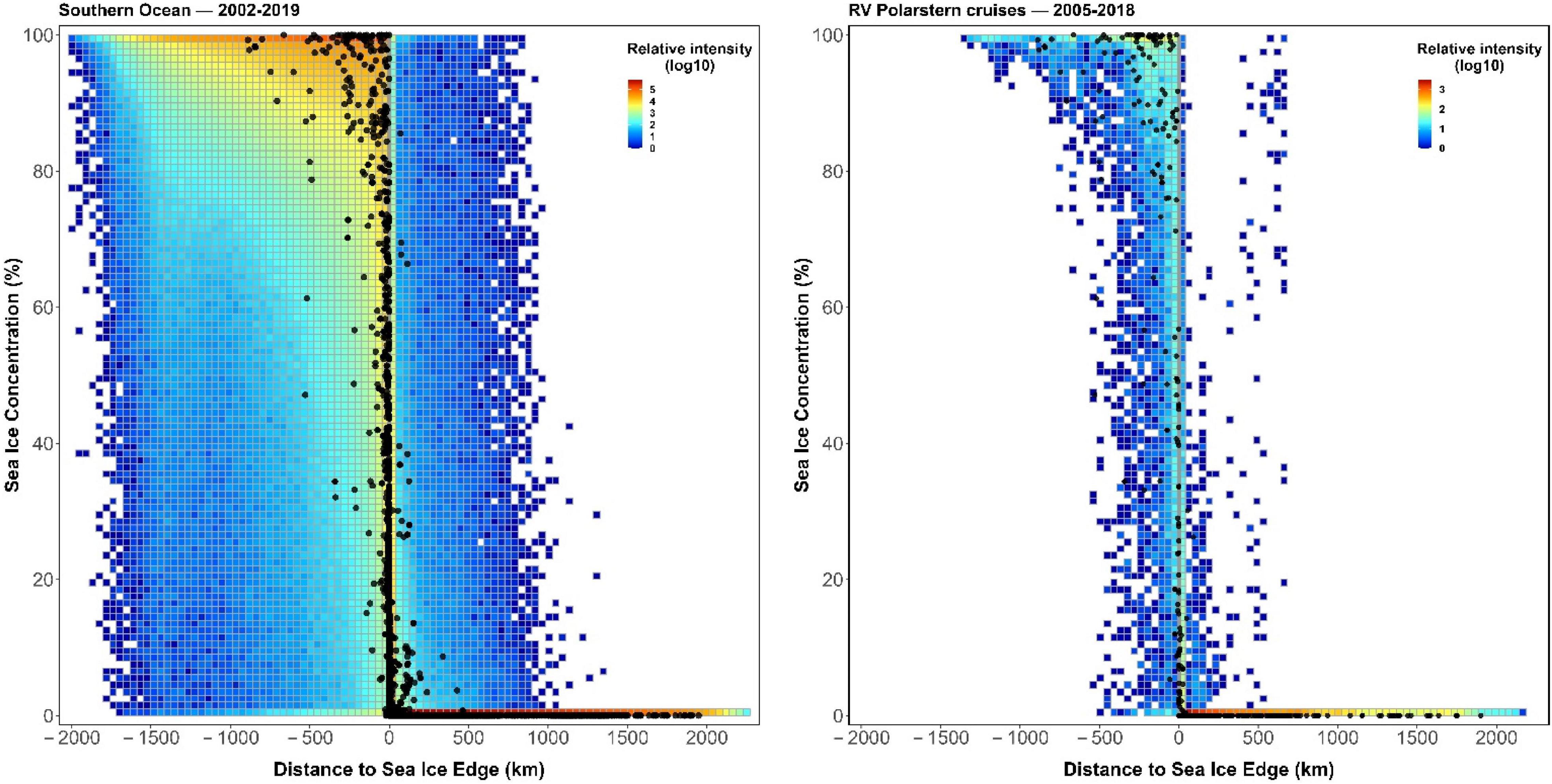
Figure 8. Combinations of environmental conditions in the Southern Ocean (SO) for daily distance to sea ice edge (SIE; x-axis) and daily sea ice concentration (SIC; y-axis). The left panel shows combinations at daily sampled 5,000 cells (2003–2010 and 2013–2019), while the right panel shows combinations on RV Polarstern expedition tracks (2005–2018). The grid color indicates the number of cells (log scale) at each combination, representing the relative intensity of environmental conditions in both datasets (white areas are for non-existing combinations). Black points represent environmental conditions at sightings of the four study species: all data used in this study in the left panel (including Polarstern data) and only Polarstern data in the right panel. The vertical gray line shows the location of the SIE (distance to SIE = 0 km). Background information only from limited cruise tracks (right plot) does not well represent combinations of long-term, year-round environmental conditions in the SO and is inevitably spatiotemporally biased towards the near/north of SIE, low SIC, and environmental conditions in summer. In contrast, the spatiotemporally sampled background information from the whole SO (left plot) shows less biases and broader coverage of environmental combinations. Polarstern sightings (black points) cover only part of the range of environmental conditions suitable for the species (right), while the use of crowdsourced data from other sources (left) covers a more comprehensive range of suitable environmental conditions. This disparity of environmental coverage is more evident for HWs observations (see Supplementary Figure 39 for species-specific observations).

Data Availability Statement

The dataset analyzed during the current study is already publicly available (details in: El-Gabbas et al., 2021a). The interactive distribution of sightings is available at this web application: https://awi-oza.shinyapps.io/BaleenWhales/. Animated videos for species-specific daily and mean weekly habitat suitability from 2003 to 2019 are publicly available at El-Gabbas et al. (2021b). Animated videos are also available as a YouTube playlist (https://youtube.com/playlist?list=PLdpRuazqmy6Es97xn0TbWi91XtLd8Wf5i).

Author Contributions

AE-G performed data curation, planned and conducted the data analysis and modeling, and wrote and edited the first draft of the manuscript. All authors delineated the study, contributed to the final manuscript’s writing, and approved the submitted version.

Funding

This work was financially supported by the German Federal Ministry of Food and Agriculture (BMEL) through the Federal Office for Agriculture and Food (BLE), Grant Number 2817HS004.

Conflict of Interest

The authors declare that the research was conducted in the absence of any commercial or financial relationships that could be construed as a potential conflict of interest.

Publisher’s Note

All claims expressed in this article are solely those of the authors and do not necessarily represent those of their affiliated organizations, or those of the publisher, the editors and the reviewers. Any product that may be evaluated in this article, or claim that may be made by its manufacturer, is not guaranteed or endorsed by the publisher.

Acknowledgments

We thank Andy Traumüller for helping in downloading environmental predictors and processing ship tracking data and all data providers for making their observation data publicly available, especially captains and nautical officers onboard RV Polarstern. We thank Hal Mueller for making sailwx data (https://www.sailwx.info/) available to us. We appreciate the fruitful discussions with Carsten F. Dormann, David Warton, and Cory Merow on how background locations should be sampled for presence-only dynamic SDMs and comments from Diego Filun, Elena Schall, Karolin Thomisch, and Irene Roca on species-specific results. This work was partially performed on the HPC computer facility of the Alfred Wegener Institute. We thank Natalja Rakowsky for technical support on the HPC computers.

Supplementary Material

The Supplementary Material for this article can be found online at: https://www.frontiersin.org/articles/10.3389/fmars.2021.802276/full#supplementary-material

Footnotes

1. ^ https://www.gbif.org/
2. ^ http://ccpo.odu.edu/Research/globec_menu.html
3. ^ https://iwc.int/sower
4. ^ https://www.awi.de/en/expedition/research-vessel-and-cutter/polarstern.html
5. ^ https://pangaea.de/
6. ^ https://copernicus.eu/
7. ^ All directions are given clockwise; i.e., eastwards.

References

Abrahms, B., Welch, H., Brodie, S., Jacox, M. G., Becker, E. A., Bograd, S. J., et al. (2019). Dynamic ensemble models to predict distributions and anthropogenic risk exposure for highly mobile species. Div. Dis. 25, 1182–1193. doi: 10.1111/ddi.12940

CrossRef Full Text | Google Scholar

Aguayo-Lobo, A. (1994). Is there a population of Minke whale that overwinter among the Antarctic sea-ice? Ser. Cient. 44, 91–98.

Google Scholar

Aiello-Lammens, M. E., Boria, R. A., Radosavljevic, A., Vilela, B., and Anderson, R. P. (2015). spThin: an R package for spatial thinning of species occurrence records for use in ecological niche models. Ecography 38, 541–545. doi: 10.1111/ecog.01132

CrossRef Full Text | Google Scholar

Ainley, D. G. (2009). A history of the exploitation of the Ross Sea. Antarctica. Polar Rec. 46, 233–243. doi: 10.1017/s003224740999009x

CrossRef Full Text | Google Scholar

Ainley, D. G., Ballard, G., and Dugger, K. M. (2006). Competition among penguins and cetaceans reveals trophic cascades in the Western Ross Sea, Antarctica. Ecology 87, 2080–2093. doi: 10.1890/0012-9658(2006)87[2080:CAPACR]2.0.CO;2

CrossRef Full Text | Google Scholar

Ainley, D. G., Dugger, K. M., Toniolo, V., and Gaffney, I. (2007). Cetacean occurrence patterns in the Amundsen and Southern Bellingshausen Sea sector, Southern Ocean. Mar. Mam. Sci. 23, 287–305. doi: 10.1111/j.1748-7692.2007.00109.x

CrossRef Full Text | Google Scholar

Ainley, D. G., Jacobs, S. S., Ribic, C. A., and Gaffney, I. (2004). Seabird distribution and oceanic features of the Amundsen and southern Bellingshausen seas. Antarct. Sci. 10, 111–123. doi: 10.1017/s0954102098000169

CrossRef Full Text | Google Scholar

Ainley, D. G., Jongsomjit, D., Ballard, G., Thiele, D., Fraser, W. R., and Tynan, C. T. (2012). Modeling the relationship of Antarctic minke whales to major ocean boundaries. Polar Biol. 35, 281–290. doi: 10.1007/s00300-011-1075-1

CrossRef Full Text | Google Scholar

Arrigo, K. R., and Van Dijken, G. L. (2003). Phytoplankton dynamics within 37 Antarctic coastal polynya systems. J. Geophys. Res. Oceans 108:1739. doi: 10.1029/2002jc001739

CrossRef Full Text | Google Scholar

Arrigo, K. R., Van Dijken, G. L., and Strong, A. L. (2015). Environmental controls of marine productivity hot spots around Antarctica. J. Geophys. Res. Oceans 120, 5545–5565. doi: 10.1002/2015jc010888

CrossRef Full Text | Google Scholar

Assis, J., Tyberghein, L., Bosch, S., Verbruggen, H., Serrao, E. A., and De Clerck, O. (2018). Bio-ORACLE v2.0: extending marine data layers for bioclimatic modelling. Glob. Ecol. Biogeogr. 27, 277–284. doi: 10.1111/geb.12693

CrossRef Full Text | Google Scholar

Atkinson, A., Hill, S. L., Pakhomov, E. A., Siegel, V., Anadon, R., Chiba, S., et al. (2017). KRILLBASE: a circumpolar database of Antarctic krill and salp numerical densities, 1926–2016. Earth Syst. Sci. Data 9, 193–210. doi: 10.5194/essd-9-193-2017

CrossRef Full Text | Google Scholar

Atkinson, A., Hill, S. L., Pakhomov, E. A., Siegel, V., Reiss, C. S., Loeb, V. J., et al. (2019). Krill (Euphausia superba) distribution contracts southward during rapid regional warming. Nat. Clim. Chang. 9, 142–149. doi: 10.1038/s41558-018-0370-z

CrossRef Full Text | Google Scholar

Atkinson, A., Siegel, V., Pakhomov, E. A., Rothery, P., Loeb, V., Ross, R. M., et al. (2008). Oceanic circumpolar habitats of Antarctic krill. Mar. Ecol. Prog. Series 362, 1–23. doi: 10.3354/meps07498

CrossRef Full Text | Google Scholar

Bamford, C. C. G., Kelly, N., Dalla Rosa, L., Cade, D. E., Fretwell, P. T., Trathan, P. N., et al. (2020). A comparison of baleen whale density estimates derived from overlapping satellite imagery and a shipborne survey. Sci. Rep. 10:12985. doi: 10.1038/s41598-020-69887-y

PubMed Abstract | CrossRef Full Text | Google Scholar

Bassoi, M., Acevedo, J., Secchi, E. R., Aguayo-Lobo, A., Dalla Rosa, L., Torres, D., et al. (2020). Cetacean distribution in relation to environmental parameters between Drake Passage and northern Antarctic Peninsula. Polar Biol. 43, 1–15. doi: 10.1007/s00300-019-02607-z

CrossRef Full Text | Google Scholar

Bateman, B. L., Vanderwal, J., and Johnson, C. N. (2012). Nice weather for bettongs: using weather events, not climate means, in species distribution models. Ecography 35, 306–314. doi: 10.1111/j.1600-0587.2011.06871.x

CrossRef Full Text | Google Scholar

Baumann-Pickering, S., Sirovic, A., Trickey, J. S., Hildebrand, J. A. Reyes Reyes, M. V., Melcon, M. L., et al. (2015). “Cetacean presence near Elephant Island, Antarctica, based on passive acoustic monitoring,” in Paper Presented at the IWC Scientific Committee SC/67a/SH18 (Cambridge: International Whaling Commission).

Google Scholar

Beekmans, B. W. P. M., Forcada, J. F., Murphy, E. J., De Baar, H. J. W., Bathmann, U., and Fleming, A. H. (2010). Generalised additive models to investigate environmental drivers of Antarctic minke whale (Balaenoptera bonaerensis) spatial density in austral summer. J. Cetac. Res. Manag. 11, 115–129.

Google Scholar

Bester, M. N., Bornemann, H., and Mcintyre, T. (2017). Antarctic marine mammals and sea ice. Sea Ice 2017, 534–555.

Google Scholar

Bestley, S., Andrews-Goff, V., Van Wijk, E., Rintoul, S. R., Double, M. C., and How, J. (2019). New insights into prime Southern Ocean forage grounds for thriving Western Australian humpback whales. Sci. Rep. 9:13988. doi: 10.1038/s41598-019-50497-2

PubMed Abstract | CrossRef Full Text | Google Scholar

Bombosch, A., Zitterbart, D. P., Van Opzeeland, I., Frickenhaus, S., Burkhardt, E., Wisz, M. S., et al. (2014). Predictive habitat modelling of humpback (Megaptera novaeangliae) and Antarctic minke (Balaenoptera bonaerensis) whales in the Southern Ocean as a planning tool for seismic surveys. Deep Sea Res. Part I 91, 101–114. doi: 10.1016/j.dsr.2014.05.017

CrossRef Full Text | Google Scholar

Bost, C. A., Cotté, C., Bailleul, F., Cherel, Y., Charrassin, J. B., Guinet, C., et al. (2009). The importance of oceanographic fronts to marine birds and mammals of the southern oceans. J. Mar. Syst. 78, 363–376. doi: 10.1016/j.jmarsys.2008.11.022

CrossRef Full Text | Google Scholar

Branch, T. A. (2007). Abundance of Antarctic blue whales south of 60°S from three complete circumpolar sets of surveys. J. Cetac. Res. Manag. 9, 253–262.

Google Scholar

Branch, T. A. (2011). Humpback whale abundance south of 60°S from three complete circumpolar sets of surveys. J. Cetac. Res. Manag. 3, 53–69. doi: 10.47536/jcrm.vi.305

CrossRef Full Text | Google Scholar

Branch, T. A., and Butterworth, D. S. (2001). Estimates of abundance south of 60°S for cetacean species sighted frequently on the 1978/79 to 1997/98 IWC/IDCR-SOWER sighting surveys. J. Cetac. Res. Manag. 3, 251–270.

Google Scholar

Branch, T. A., Matsuoka, K., and Miyashita, T. (2004). Evidence for increases in Antarctic blue whales based on Bayesian modelling. Mar. Mamm. Sci. 20, 726–754. doi: 10.1111/j.1748-7692.2004.tb01190.x

CrossRef Full Text | Google Scholar

Branch, T. A., Stafford, K. M., Palacios, D. M., Allison, C., Bannister, J. L., Burton, C. L. K., et al. (2007). Past and present distribution, densities and movements of blue whales Balaenoptera musculus in the Southern Hemisphere and northern Indian Ocean. Mamm. Rev. 37, 116–175. doi: 10.1111/j.1365-2907.2007.00106.x

CrossRef Full Text | Google Scholar

Brierley, A. S., Fernandes, P. G., Brandon, M. A., Armstrong, F., Millard, N. W., Mcphail, S. D., et al. (2002). Antarctic krill under sea ice: elevated abundance in a narrow band just south of ice edge. Science 295, 1890–1892. doi: 10.1126/science.1068574

PubMed Abstract | CrossRef Full Text | Google Scholar

Brown, M. R., Corkeron, P. J., Hale, P. T., Schultz, K. W., and Bryden, M. M. (1995). Evidence for a sex-segregated migration in the humpback whale (Megaptera novaeangliae). Proc. Biol. Sci. 259, 229–234. doi: 10.1098/rspb.1995.0034

PubMed Abstract | CrossRef Full Text | Google Scholar

Buchan, S. J., Balcazar-Cabrera, N., and Stafford, K. M. (2020). Seasonal acoustic presence of blue, fin, and minke whales off the Juan Fernández Archipelago, Chile (2007–2016). Mar. Biodiv. 50:3. doi: 10.1007/s12526-020-01087-3

CrossRef Full Text | Google Scholar

Burkhardt, E. (2009a). Whale sightings during POLARSTERN cruise ANT-XXIII/6. Alfred Wegener Institute, Helmholtz Centre for Polar and Marine Research, Bremerhaven. PANGAEA 2009:729034. doi: 10.1594/PANGAEA.729034

CrossRef Full Text | Google Scholar

Burkhardt, E. (2009b). Whale sightings during POLARSTERN cruise ANT-XXIII/7. Alfred Wegener Institute, Helmholtz Centre for Polar and Marine Research, Bremerhaven. PANGAEA 2009:729035. doi: 10.1594/PANGAEA.729035

CrossRef Full Text | Google Scholar

Burkhardt, E. (2013b). Whale sightings during POLARSTERN cruise ANT-XXVIII/4. Alfred Wegener Institute, Helmholtz Centre for Polar and Marine Research, Bremerhaven. PANGAEA 2013:819863. doi: 10.1594/PANGAEA.819863

CrossRef Full Text | Google Scholar

Burkhardt, E. (2013a). Whale sightings during POLARSTERN cruise ANT-XXIX/2. Alfred Wegener Institute, Helmholtz Centre for Polar and Marine Research, Bremerhaven. PANGAEA 2013:819866. doi: 10.1594/PANGAEA.819866

CrossRef Full Text | Google Scholar

Burkhardt, E., and Lanfredi, C. (2012). “Fall feeding aggregations of fin whales off Elephant Island (Antarctica),” in Paper Presented at the IWC Scientific Committee SC/64/SH9. Available online at: https://epic.awi.de/id/eprint/30452/1/SC-64-SH9_corrected_may22.pdf

Google Scholar

Burkhardt, E., Van Opzeeland, I., Cisewski, B., Mattmüller, R., Meister, M., Schall, E., et al. (2021). Seasonal and diel cycles of fin whale acoustic occurrence near Elephant Island, Antarctica. R. Soc. Open Sci. 8:201142. doi: 10.1098/rsos.201142

PubMed Abstract | CrossRef Full Text | Google Scholar

Cai, W., Borlace, S., Lengaigne, M., Van Rensch, P., Collins, M., Vecchi, G., et al. (2014). Increasing frequency of extreme El Niño events due to greenhouse warming. Nat. Clim. Change 4, 111–116. doi: 10.1038/nclimate2100

CrossRef Full Text | Google Scholar

Calderan, S. V., Black, A., Branch, T. A., Collins, M. A., Kelly, N., Leaper, R., et al. (2020). South Georgia blue whales five decades after the end of whaling. Endanger. Species Res. 43, 359–373. doi: 10.3354/esr01077

CrossRef Full Text | Google Scholar

Clapham, P., and Baker, C. S. (2002). Modern whaling. Encycloped. Mar. Mamm. 2002, 1328–1332.

Google Scholar

Clapham, P. J., Aguilar, A., and Hatch, L. T. (2008). Determining spatial and temporal scales for management: lessons from whaling. Mar. Mamm. Sci. 24, 183–201. doi: 10.1111/j.1748-7692.2007.00175.x

CrossRef Full Text | Google Scholar

Constable, A. J., Nicol, S., and Strutton, P. G. (2003). Southern Ocean productivity in relation to spatial and temporal variation in the physical environment. J. Geophys. Res. Oceans 108:1270. doi: 10.1029/2001jc001270

CrossRef Full Text | Google Scholar

Cooke, J. G. (2018a). Balaenoptera musculus ssp. intermedia. The IUCN Red List of Threatened Species. doi: 10.2305/IUCN.UK.2018-2.RLTS.T41713A50226962.en

PubMed Abstract | CrossRef Full Text | Google Scholar

Cooke, J. G. (2018b). Balaenoptera physalus. The IUCN Red List of Threatened Species. doi: 10.2305/IUCN.UK.2018-2.RLTS.T2478A50349982.en

PubMed Abstract | CrossRef Full Text | Google Scholar

Cooke, J. G. (2018c). Megaptera novaeangliae. The IUCN Red List of Threatened Species. doi: 10.2305/IUCN.UK.2018-2.RLTS.T13006A50362794.en

PubMed Abstract | CrossRef Full Text | Google Scholar

Cooke, J. G., Zerbini, A. N., and Taylor, B. L. (2018). Balaenoptera bonaerensis. The IUCN Red List of Threatened Species. doi: 10.2305/IUCN.UK.2018-1.RLTS.T2480A50350661.en

PubMed Abstract | CrossRef Full Text | Google Scholar

Curtice, C., Johnston, D. W., Ducklow, H., Gales, N., Halpin, P. N., and Friedlaender, A. S. (2015). Modeling the spatial and temporal dynamics of foraging movements of humpback whales (Megaptera novaeangliae) in the Western Antarctic Peninsula. Move. Ecol. 3:13. doi: 10.1186/s40462-015-0041-x

PubMed Abstract | CrossRef Full Text | Google Scholar

Cuzin-Roudy, J., Irisson, J.-O., Penot, F., Kawaguchi, S., and Vallet, C. (2014). Southern Ocean Euphausiids. Biogeogr. Atlas Souther. Ocean 2014, 309–320.

Google Scholar

Dalla Rosa, L., Secchi, E. R., Maia, Y. G., Zerbini, A. N., and Heide-Jørgensen, M. P. (2008). Movements of satellite-monitored humpback whales on their feeding ground along the Antarctic Peninsula. Polar Biol. 31, 771–781. doi: 10.1007/s00300-008-0415-2

CrossRef Full Text | Google Scholar

Daly, K. L., and Macaulay, M. C. (1988). Abundance and distribution of krill in the ice edge zone of the Weddell Sea, austral spring 1983. Deep Sea Res. Part I: Oceanogr. Res. Papers 35, 21–41. doi: 10.1016/0198-0149(88)90055-6

CrossRef Full Text | Google Scholar

Dominello, T., and Širović, A. (2016). Seasonality of Antarctic minke whale (Balaenoptera bonaerensis) calls off the western Antarctic Peninsula. Mar. Mamm. Sci. 32, 826–838. doi: 10.1111/mms.12302

CrossRef Full Text | Google Scholar

Doney, S. C., Ruckelshaus, M., Duffy, J. E., Barry, J. P., Chan, F., English, C. A., et al. (2012). Climate change impacts on marine ecosystems. Annu. Rev. Mar. Sci. 4, 11–37. doi: 10.1146/annurev-marine-041911-111611

PubMed Abstract | CrossRef Full Text | Google Scholar

Double, M. C., Miller, B. S., Leaper, R., Olson, P., Cox, M. J., Miller, E., et al. (2015). “Cruise report on blue whale research from the NZ/Aus Antarctic ecosystems voyage 2015 of the Southern Ocean Research Partnership,” in Paper Presented at the IWC Scientific Committee SC/66a/SH/7 (Cambridge: International Whaling Commission).

Google Scholar

Druskat, A., Ghosh, R., Castrillon, J., and Bengtson Nash, S. M. (2019). Sex ratios of migrating southern hemisphere humpback whales: A new sentinel parameter of ecosystem health. Marine Env. Res. 151:104749. doi: 10.1016/j.marenvres.2019.104749

PubMed Abstract | CrossRef Full Text | Google Scholar

Dziak, R. P., Bohnenstiehl, D. R., Stafford, K. M., Matsumoto, H., Park, M., Lee, W. S., et al. (2015). Sources and levels of ambient ocean sound near the Antarctic Peninsula. PLoS One 10:e0123425. doi: 10.1371/journal.pone.0123425

PubMed Abstract | CrossRef Full Text | Google Scholar

El-Gabbas, A., and Dormann, C. F. (2018). Improved species-occurrence predictions in data-poor regions: using large-scale data and bias correction with down-weighted Poisson regression and Maxent. Ecography 41, 1161–1172. doi: 10.1111/ecog.03149

CrossRef Full Text | Google Scholar

El-Gabbas, A., Van Opzeeland, I., Burkhardt, E., and Boebel, O. (2021a). Static species distribution models in the marine realm: The case of baleen whales in the Southern Ocean. Div. Distribut. 27, 1536–1552. doi: 10.1111/ddi.13300

CrossRef Full Text | Google Scholar

El-Gabbas, A. Van Opzeeland, I., Burkhardt, E., and Boebel, O. (2021b). Year-Round Habitat Suitability of Baleen Whales in the Southern Ocean. London: Figshare Media. doi: 10.6084/m9.figshare.16611556

CrossRef Full Text | Google Scholar

Elith, J., and Leathwick, J. R. (2009). Species distribution models: ecological explanation and prediction across space and time. Annu. Rev. Ecol. Evol. Syst. 40, 677–697. doi: 10.1146/annurev.ecolsys.110308.120159

CrossRef Full Text | Google Scholar

Elith, J., Phillips, S. J., Hastie, T., Dudík, M., Chee, Y. E., and Yates, C. J. (2011). A statistical explanation of MaxEnt for ecologists. Diversity and Distributions 17, 43–57. doi: 10.1111/j.1472-4642.2010.00725.x

CrossRef Full Text | Google Scholar

Engel, M. H., and Martin, A. R. (2009). Feeding grounds of the western South Atlantic humpback whale population. Mar. Mamm. Sci. 25, 964–969. doi: 10.1111/j.1748-7692.2009.00301.x

CrossRef Full Text | Google Scholar

Ensor, P., Komiya, H., Beasley, I., Fukutome, K., Olson, P., and Tsuda, Y. (2007). “2006–2007 International Whaling Commission-Southern Ocean Whale and Ecosystem Research (IWC-SOWER) cruise,” in Paper Presented at the IWC Scientific Committee SC/59/IA1 (Cambridge: International Whaling Commission).

Google Scholar

Ensor, P. H. (1989). “Minke whales in the pack ice zone, East Antarctica, during the period of maximum annual ice extent,” in Paper Presented at the IWC Scientific Committee SC/40/Mi3 (Cambridge: International Whaling Commission).

Google Scholar

Erickson, A. W. (1984). Aerial census of seals, whales, and penguins in the pack ice of the northwestern Weddell Sea, November 1983. Antarc. J. U S 19, 121–124.

Google Scholar

Fernandez, M., Yesson, C., Gannier, A., Miller, P. I., and Azevedo, J. M. N. (2017). The importance of temporal resolution for niche modelling in dynamic marine environments. J. Biogeogr. 44, 2816–2827. doi: 10.1111/jbi.13080

CrossRef Full Text | Google Scholar

Fick, S. E., and Hijmans, R. J. (2017). WorldClim 2: new 1−km spatial resolution climate surfaces for global land areas. Internat. J. Climatol. 37, 4302–4315. doi: 10.1002/joc.5086

CrossRef Full Text | Google Scholar

Filun, D., Thomisch, K., Boebel, O., Brey, T., Sirovic, A., Spiesecke, S., et al. (2020). Frozen verses: Antarctic minke whales (Balaenoptera bonaerensis) call predominantly during austral winter. R. Soc. Open Sci. 7:192112. doi: 10.1098/rsos.192112

PubMed Abstract | CrossRef Full Text | Google Scholar

Frasier, K. E., Garrison, L. P., Soldevilla, M. S., Wiggins, S. M., and Hildebrand, J. A. (2021). Cetacean distribution models based on visual and passive acoustic data. Sci. Rep. 11:8240. doi: 10.1038/s41598-021-87577-1

PubMed Abstract | CrossRef Full Text | Google Scholar

Friedlaender, A. S., Halpin, P. N., Qian, S. S., Lawson, G. L., Wiebe, P. H., Thiele, D., et al. (2006). Whale distribution in relation to prey abundance and oceanographic processes in shelf waters of the Western Antarctic Peninsula. Marine Ecology Progress Series 317, 297–310. doi: 10.3354/meps317297

CrossRef Full Text | Google Scholar

Friedlaender, A. S., Johnston, D. W., Fraser, W. R., Burns, J., Patrick, N. H., and Costa, D. P. (2011). Ecological niche modeling of sympatric krill predators around Marguerite Bay, Western Antarctic Peninsula. Deep Sea Res. Part II 58, 1729–1740. doi: 10.1016/j.dsr2.2010.11.018

CrossRef Full Text | Google Scholar

Friedlaender, A. S., Joyce, T., Johnston, D. W., Read, A. J., Nowacek, D. P., Goldbogen, J. A., et al. (2021). Sympatry and resource partitioning between the largest krill consumers around the Antarctic Peninsula. Mar. Ecol. Prog. Series 669, 1–16. doi: 10.3354/meps13771

CrossRef Full Text | Google Scholar

Friedlaender, A. S., Lawson, G. L., and Halpin, P. N. (2009). Evidence of resource partitioning between humpback and minke whales around the western Antarctic Peninsula. Mar. Mamm. Sci. 25, 402–415. doi: 10.1111/j.1748-7692.2008.00263.x

CrossRef Full Text | Google Scholar

Friedlaender, A. S., Tyson, R. B., Stimpert, A. K., Read, A. J., and Nowacek, D. P. (2013). Extreme diel variation in the feeding behavior of humpback whales along the western Antarctic Peninsula during autumn. Mar. Ecol. Prog. Ser. 494, 281–289. doi: 10.3354/meps10541

CrossRef Full Text | Google Scholar

Gedamke, J., and Robinson, S. M. (2010). Acoustic survey for marine mammal occurrence and distribution off East Antarctica (30-80°E) in January-February 2006. Deep Sea Res. Part II 57, 968–981. doi: 10.1016/j.dsr2.2008.10.042

CrossRef Full Text | Google Scholar

Gill, P. C., and Thiele, D. (1997). A winter sighting of killer whales (Orcinus orca) in Antarctic sea ice. Polar Biol. 17, 401–404. doi: 10.1007/s003000050134

CrossRef Full Text | Google Scholar

Gilles, A., Viquerat, S., Becker, E. A., Forney, K. A., Geelhoed, S. C. V., Haelters, J., et al. (2016). Seasonal habitat-based density models for a marine top predator, the harbor porpoise, in a dynamic environment. Ecosphere 7:e01367. doi: 10.1002/ecs2.1367

CrossRef Full Text | Google Scholar

Guillera-Arroita, G., Lahoz-Monfort, J. J., Elith, J., and O’hara, R. B. (2014). Maxent is not a presence-absence method: a comment on Thibaudet al. Methods Ecol. Evol. 5, 1192–1197. doi: 10.1111/2041-210x.12252

CrossRef Full Text | Google Scholar

Guisan, A., Tingley, R., Baumgartner, J. B., Naujokaitis-Lewis, I., Sutcliffe, P. R., Tulloch, A. I., et al. (2013). Predicting species distributions for conservation decisions. Ecol. Lett. 16, 1424–1435. doi: 10.1111/ele.12189

PubMed Abstract | CrossRef Full Text | Google Scholar

Gutt, J., Bertler, N., Bracegirdle, T. J., Buschmann, A., Comiso, J., Hosie, G., et al. (2015). The Southern Ocean ecosystem under multiple climate change stresses - an integrated circumpolar assessment. Glob. Change Biol. 21, 1434–1453. doi: 10.1111/gcb.12794

PubMed Abstract | CrossRef Full Text | Google Scholar

Hakamada, T., and Matsuoka, K. (2013). “Estimates of abundance and abundance trend of the humpback whale in areas IIIE-VIW, south of 60°S, based on JARPA and JARPAII sighting data (1989/90-2008/09),” in Paper Presented at the IWC Scientific Committee SC/F14/J04 (Cambridge: International Whaling Commission).

Google Scholar

Halpin, P., Read, A., Fujioka, E., Best, B., Donnelly, B., Hazen, L., et al. (2009). OBIS-SEAMAP: the world data center for marine mammal, sea bird, and sea turtle distributions. Oceanography 22, 104–115. doi: 10.5670/oceanog.2009.42

CrossRef Full Text | Google Scholar

Harmer, S. F. (1931). Southern whaling. Proc. Linn. Soc. Lond. 142, 85–163. doi: 10.1111/j.1095-8312.1931.tb01464.x

CrossRef Full Text | Google Scholar

Hazen, E. L., Palacios, D. M., Forney, K. A., Howell, E. A., Becker, E., Hoover, A. L., et al. (2017). WhaleWatch: a dynamic management tool for predicting blue whale density in the California Current. J. Appl. Ecol. 54, 1415–1428. doi: 10.1111/1365-2664.12820

CrossRef Full Text | Google Scholar

Herr, H., Kelly, N., Dorschel, B., Huntemann, M., Kock, K. H., Lehnert, L. S., et al. (2019). Aerial surveys for Antarctic minke whales (Balaenoptera bonaerensis) reveal sea ice dependent distribution patterns. Ecol. Evol. 9, 5664–5682. doi: 10.1002/ece3.5149

PubMed Abstract | CrossRef Full Text | Google Scholar

Herr, H., Viquerat, S., Siegel, V., Kock, K. H., Dorschel, B., Huneke, W. G. C., et al. (2016). Horizontal niche partitioning of humpback and fin whales around the West Antarctic Peninsula: evidence from a concurrent whale and krill survey. Polar Biol. 39, 799–818. doi: 10.1007/s00300-016-1927-9

CrossRef Full Text | Google Scholar

Hinton, M. A. C. (1915). Report on the Papers Left by the Late Major Barrett- Hamilton, Relating to the Whales of South Georgia. Inter-Departmental Committee on Whaling and the Protection of Whales (Appendix VII). Colonial Office Miscellaneous No. 298. London: Crown Agents for the Colonies, 69–193.

Google Scholar

Hjort, J., Lie, J., and Ruud, J. T. (1932). Norwegian pelagic whaling in the Antarctic. Hvalradet Skrifter 3, 1–37.

Google Scholar

Hortal, J., De Bello, F., Diniz-Filho, J. A. F., Lewinsohn, T. M., Lobo, J. M., and Ladle, R. J. (2015). Seven shortfalls that beset large-scale knowledge of biodiversity. Annu. Rev. Ecol. Evol. Syst. 46, 523–549. doi: 10.1146/annurev-ecolsys-112414-054400

CrossRef Full Text | Google Scholar

Horwood, J. W. (1986). The distribution of the southern blue whale in relation to recent estimates and abundance. Sci. Rep. Whales Res. Inst. 37, 155–165.

Google Scholar

Hunt, G. L., Drinkwater, K. F., Arrigo, K., Berge, J., Daly, K. L., Danielson, S., et al. (2016). Advection in polar and sub-polar environments: Impacts on high latitude marine ecosystems. Prog. Oceanogr. 149, 40–81. doi: 10.1016/j.pocean.2016.10.004

CrossRef Full Text | Google Scholar

Ichii, T. (1990). Distribution of Antarctic krill concentrations exploited by Japanese krill trawlers and minke whales. Proc. NIPR Symp. Polar Biol. 3, 36–56.

Google Scholar

Ingenloff, K., Peterson, A. T., and Peres-Neto, P. (2020). Incorporating time into the traditional correlational distributional modelling framework: A proof-of-concept using the Wood Thrush Hylocichla mustelina. Methods in Ecology and Evolution 12, 311–321. doi: 10.1111/2041-210x.13523

CrossRef Full Text | Google Scholar

Isoda, T., Katsumata, T., Yamaguchi, F., Ohkoshi, C., and Matsuoka, K. (2020). “Results of the Japanese abundance and stock structure survey in the Antarctic (JASS-A) during the 2019/20 austral summer season,” in Paper Presented at the IWC Scientific Committee SC/68B/ASI/17 (Cambridge: International Whaling Commission).

Google Scholar

Isoda, T., Konishi, K., Yamaguchi, F., Kawabe, S., Moriyama, R., Kasai, H., et al. (2017). “Results of the NEWREP-A dedicated sighting survey during the 2016/17 austral summer season,” in Paper Presented at the IWC Scientific Committee SC/67A/ASI/07 (Cambridge: International Whaling Commission).

Google Scholar

Jewell, R., Thomas, L., Harris, C. M., Kaschner, K., Wiff, R., Hammond, P. S., et al. (2012). Global analysis of cetacean line-transect surveys: detecting trends in cetacean density. Mar. Ecol. Prog. Series 453, 227–240. doi: 10.3354/meps09636

CrossRef Full Text | Google Scholar

Johnston, D. W., Friedlaender, A. S., Read, A. J., and Nowacek, D. P. (2012). Initial density estimates of humpback whales Megaptera novaeangliae in the inshore waters of the western Antarctic Peninsula during the late autumn. Endang. Species Res. 18, 63–71. doi: 10.3354/esr00395

CrossRef Full Text | Google Scholar

Joiris, C. R., and Dochy, O. (2013). A major autumn feeding ground for fin whales, southern fulmars and grey-headed albatrosses around the South Shetland Islands. Antarctica. Polar Biology 36, 1649–1658. doi: 10.1007/s00300-013-1383-8

CrossRef Full Text | Google Scholar

Kasamatsu, F., Ensor, P., Joyce, G. G., and Kimura, N. (2000a). Distribution of minke whales in the Bellingshausen and Amundsen Seas (60°W–120°W), with special reference to environmental/physiographic variables. Fish. Oceanogr. 9, 214–223. doi: 10.1046/j.1365-2419.2000.00137.x

CrossRef Full Text | Google Scholar

Kasamatsu, F., Matsuoka, K., and Hakamada, T. (2000b). Interspecific relationships in density among the whale community in the Antarctic. Polar Biol. 23, 466–473. doi: 10.1007/s003009900107

CrossRef Full Text | Google Scholar

Kasamatsu, F., Hembree, D., Joyce, G., Tsunoda, L., Rowlett, R., and Nakano, T. (1988). “Distribution of cetacean sightings in the Antarctic: results obtained from the IWC/IDCR minke whale assessment cruises, 1978/79 to 1983/84,” in Paper Presented at the IWC Scientific Committee SC/39/OI0 (Cambridge: International Whaling Commission).

Google Scholar

Kasamatsu, F., Joyce, G. G., Ensor, P., and Mermoz, J. (1996). “Current occurrence of baleen whales in Antarctic waters,” in Paper Presented at the IWC Scientific Committee SC/47/SH4 (Cambridge: International Whaling Commission).

Google Scholar

Kaschner, K., Watson, R., Trites, A. W., and Pauly, D. (2006). Mapping world-wide distributions of marine mammal species using a relative environmental suitability (RES) model. Mar. Ecol. Prog. Series 316, 285–310. doi: 10.3354/meps316285

CrossRef Full Text | Google Scholar

Kellogg, R. (1929). What is known of the migration of some of the whalebone whales. Annu. Rep. Smiths. Inst. 1928, 467–494.

Google Scholar

Kemp, S., and Bennett, A. G. (1932). On the distribution and movements of whales on the South Georgia and South Shetland whaling grounds. Discov. Rep. 7, 167–190.

Google Scholar

Kennedy, A. S., Carroll, E. L., Baker, C. S., Bassoi, M., Buss, D., Collins, M. A., et al. (2020). “Whales return to the epicentre of whaling? Preliminary results from the 2020 cetacean survey at South Georgia (Islas Georgias del Sur),” in Paper Presented at the IWC Scientific Committee SC/68B/CMP/22 (Cambridge: International Whaling Commission).

Google Scholar

Konishi, K., Isoda, T., Bando, T., Minamikawa, S., and Kleivane, L. (2020). Antarctic minke whales find ice gaps along the ice edge in foraging grounds of the Indo-Pacific sector (60° E and 140° E) of the Southern Ocean. Polar Biol. 43, 343–357. doi: 10.1007/s00300-020-02638-x

CrossRef Full Text | Google Scholar

Labrousse, S., Williams, G., Tamura, T., Bestley, S., Sallee, J. B., Fraser, A. D., et al. (2018). Coastal polynyas: Winter oases for subadult southern elephant seals in East Antarctica. Sci. Rep. 8:3183. doi: 10.1038/s41598-018-21388-9

PubMed Abstract | CrossRef Full Text | Google Scholar

Laws, R. M. (1977a). Seals and whales of the Southern Ocean. Philosoph. Transact. R. Soc. B 279, 81–96. doi: 10.1098/rstb.1977.0073

CrossRef Full Text | Google Scholar

Laws, R. M. (1977b). “The significance of vertebrates in the Antarctic marine ecosystem,” in Adaptations within Antarctic ecosystems, ed. G. A. Llano (Washington, D.C: Smithsonian Institution Press), 411–438.

Google Scholar

Leaper, R., and Miller, C. (2011). Management of Antarctic baleen whales amid past exploitation, current threats and complex marine ecosystems. Antarc. Sci. 23, 503–529. doi: 10.1017/s0954102011000708

CrossRef Full Text | Google Scholar

Lee, J. F., Friedlaender, A. S., Oliver, M. J., and Deliberty, T. L. (2017). Behavior of satellite-tracked Antarctic minke whales (Balaenoptera bonaerensis) in relation to environmental factors around the western Antarctic Peninsula. Anim. Biotele. 5:23. doi: 10.1186/s40317-017-0138-7

CrossRef Full Text | Google Scholar

Leroy, E. C., Samaran, F., Bonnel, J., and Royer, J. Y. (2016). Seasonal and diel vocalization patterns of Antarctic blue whale (Balaenoptera musculus intermedia) in the Southern Indian Ocean: a multi-year and multi-site study. PLoS One 11:e0163587. doi: 10.1371/journal.pone.0163587

PubMed Abstract | CrossRef Full Text | Google Scholar

Leroy, E. C., Samaran, F., Stafford, K. M., Bonnel, J., and Royer, J. Y. (2018). Broad-scale study of the seasonal and geographic occurrence of blue and fin whales in the Southern Indian Ocean. Endanger. Species Res. 37, 289–300. doi: 10.3354/esr00927

CrossRef Full Text | Google Scholar

Liu, C., White, M., Newell, G., and Pearson, R. (2013). Selecting thresholds for the prediction of species occurrence with presence-only data. J. Biogeogr. 40, 778–789. doi: 10.1111/jbi.12058

CrossRef Full Text | Google Scholar

Loeb, V. J., and Santora, J. A. (2015). Climate variability and spatiotemporal dynamics of five Southern Ocean krill species. Prog. Oceanogr. 134, 93–122. doi: 10.1016/j.pocean.2015.01.002

CrossRef Full Text | Google Scholar

Mackintosh, N. A. (1942). The southern stocks of whalebone whales. Discov. Rep. 22, 197–300.

Google Scholar

Matsuoka, K., and Hakamada, T. (2014). “Estimates of abundance and abundance trend of the blue, fin and southern right whales in the Antarctic areas IIIE-VIW, south of 60°S, based on JARPA and JARPAII sighting data (1989/90-2008/09),” in Paper Presented at the IWC Scientific Committee SC/F14/J05 (Cambridge: International Whaling Commission).

Google Scholar

Matsuoka, K., and Hakamada, T. (2020). Density distribution of several major whale species in the Indo-Pacific region of Antarctic using JARPA and JARPAII sighting data obtained through 1987/88 – 2008/09 season. Cetac. Populat. Stud. 2, 15–38.

Google Scholar

Matsuoka, K., Hakamada, T., Kiwada, H., Murase, H., and Nishiwaki, S. (2006a). “Distributions and standardized abundance estimates for humpback, fin and blue whales in the Antarctic areas IIIE, IV, V and VIW (35°E–145°W), south of 60°S,” in Paper Presented at the IWC Scientific Committee SC/D06/J71 (Cambridge: International Whaling Commission).

Google Scholar

Matsuoka, K., Hakamada, T., Kiwada, H., Murase, H., and Nishiwaki, S. (2006b). “Updated distribution and abundance estimates of humpback whales in the Antarctic areas IV and V (70°E–170°W),” in Paper Presented at the IWC Scientific Committee SC/58/SH21 (Cambridge: International Whaling Commission).

Google Scholar

Matsuoka, K., Watanabe, T., Ichii, T., Shimada, H., and Nishiwaki, S. (2003). “Large whale distributions (south of 60°S, 35°E-130°E) in relation to the southern boundary of the Antarctic Circumpolar Current,” in Antarctic biology in a global context, eds A. H. L. Huiskes, W. W. C. Gieskes, J. Rozema, R. M. L. Schorno, S. M. Van Der Vies, and W. J. Wolff (Leiden: Backhuys Publishers).

Google Scholar

Matthews, L. H. (1937). The humpback whale, Megaptera Nodosa. Discov. Rep. 17, 7–92.

Google Scholar

Maxwell, S. M., Hazen, E. L., Lewison, R. L., Dunn, D. C., Bailey, H., Bograd, S. J., et al. (2015). Dynamic ocean management: defining and conceptualizing real-time management of the ocean. Mar. Policy 58, 42–50. doi: 10.1016/j.marpol.2015.03.014

CrossRef Full Text | Google Scholar

Mckay, S., Sirovic, A., Thiele, D., Abery, N. W., Chester, E. T., Hildebrand, J., et al. (2004). “Combining acoustic, sighting survey and sea ice data to investigate the seasonal presence of humpback whales, Megaptera novaeangliae, in the Western Antarctic Peninsula,” in Paper Presented at the IWC Scientific Committee SC/56/E26 (Cambridge: International Whaling Commission).

Google Scholar

Mellinger, D. K., Stafford, K. M., Moore, S. E., Dziak, R. P., and Matsumoto, H. (2007). An Overview of Fixed Passive Acoustic Observation Methods for Cetaceans. Oceanography 20, 36–45. doi: 10.5670/oceanog.2007.03

CrossRef Full Text | Google Scholar

Menegotto, A., and Rangel, T. F. (2018). Mapping knowledge gaps in marine diversity reveals a latitudinal gradient of missing species richness. Nat. Comm. 9:4713. doi: 10.1038/s41467-018-07217-7

PubMed Abstract | CrossRef Full Text | Google Scholar

Merow, C., Smith, M. J., and Silander, J. A. (2013). A practical guide to MaxEnt for modeling species’ distributions: what it does, and why inputs and settings matter. Ecography 36, 1058–1069. doi: 10.1111/j.1600-0587.2013.07872.x

CrossRef Full Text | Google Scholar

Meynecke, J.-O., and Meager, J. J. (2016). Understanding strandings: 25 years of humpback whale (Megaptera novaeangliae) strandings in Queensland, Australia. J. Coast. Res. 75, 897–901. doi: 10.2112/si75-180.1

CrossRef Full Text | Google Scholar

Meynecke, J. O., Seyboth, E., De Bie, J., Menzel Barraqueta, J. L., Chama, A., Prakash Dey, S., et al. (2020). Responses of humpback whales to a changing climate in the Southern Hemisphere: priorities for research efforts. Mar. Ecol. 41:12616. doi: 10.1111/maec.12616

CrossRef Full Text | Google Scholar

Milanesi, P., Della Rocca, F., and Robinson, R. A. (2020). Integrating dynamic environmental predictors and species occurrences: toward true dynamic species distribution models. Ecol. Evol. 10, 1087–1092. doi: 10.1002/ece3.5938

PubMed Abstract | CrossRef Full Text | Google Scholar

Miller, B. S., Barlow, J., Calderan, S., Collins, K., Leaper, R., Olson, P., et al. (2015). Validating the reliability of passive acoustic localisation: a novel method for encountering rare and remote Antarctic blue whales. Endanger. Species Res. 26, 257–269. doi: 10.3354/esr00642

CrossRef Full Text | Google Scholar

Miller, B. S., Calderan, S., Miller, E. J. Široviæ, A., Stafford, K. M., Bell, E., et al. (2019). “A passive acoustic survey for marine mammals conducted during the 2019 Antarctic voyage on Euphausiids and Nutrient Recycling in Cetacean Hotspots (ENRICH),” in Proceedings of the ACOUSTICS 2019, Cape Schanck, VIC.

Google Scholar

Miller, B. S., Group, I. S. S. A. T. W., Balcazar, N., Nieukirk, S., Leroy, E. C., Aulich, M., et al. (2021). An open access dataset for developing automated detectors of Antarctic baleen whale sounds and performance evaluation of two commonly used detectors. Sci. Rep. 11:806. doi: 10.1038/s41598-020-78995-8

PubMed Abstract | CrossRef Full Text | Google Scholar

Miller, B. S., Miller, E., Calderan, S., Leaper, R., Stafford, K., Sirovic, A., et al. (2017). “Circumpolar acoustic mapping of endangered Southern Ocean Whales: voyage report and preliminary results for the 2016/17 Antarctic circumnavigation expedition,” in Paper Presented at the IWC Scientific Committee SC/67A/SH03 (Cambridge: International Whaling Commission).

Google Scholar

Miller, E. J., Potts, J. M., Cox, M. J., Miller, B. S., Calderan, S., Leaper, R., et al. (2019). The characteristics of krill swarms in relation to aggregating Antarctic blue whales. Sci. Rep. 9:16487. doi: 10.1038/s41598-019-52792-4

PubMed Abstract | CrossRef Full Text | Google Scholar

Mogoe, T., Isoda, T., Yoshida, T., Nakai, K., Kanbayashi, J., Ono, K., et al. (2017). “Results of the second biological field survey of NEWREP-A during the 2016/17 austral summer season,” in Paper Presented at the IWC Scientific Committee SC/67A/SCSP0 (Cambridge: International Whaling Commission).

Google Scholar

Mogoe, T., Matsuoka, K., Nakai, K., Sato, H., Sato, T., Tsunekawa, M., et al. (2016). “Results of biological sampling of Antarctic minke whale during the first field survey of NEWREP-A in area V during the 2015/16 austral summer season,” in Paper Presented at the IWC Scientific Committee SC/66b/SP07 (Cambridge: International Whaling Commission).

Google Scholar

Mogoe, T., Yoshimura, I., Katsumata, T., Ohkoshi, C., Bando, T., and Matsuoka, K. (2019). “Results of the NEWREP-A dedicated sighting survey during the 2018/19 austral summer season,” in Paper Presented at the IWC Scientific Committee SC/68a/ASI02 (Cambridge: International Whaling Commission).

Google Scholar

Moore, M. J., Berrow, S. D., Jensen, B. A., Carr, P., Sears, R., Rowntree, V. J., et al. (1999). Relative abundance of large whales around South Georgia (1979-1998). Mar. Mamm. Sci. 15, 1287–1302. doi: 10.1111/j.1748-7692.1999.tb00891.x

CrossRef Full Text | Google Scholar

Murase, H., Kitakado, T., Hakamada, T., Matsuoka, K., Nishiwaki, S., and Naganobu, M. (2013). Spatial distribution of Antarctic minke whales (Balaenoptera bonaerensis) in relation to spatial distributions of krill in the Ross Sea, Antarctica. Fish. Oceanogr. 22, 154–173. doi: 10.1111/fog.12011

CrossRef Full Text | Google Scholar

Murase, H., Matsuoka, K., Ichii, T., and Nishiwaki, S. (2002). Relationship between the distribution of euphausiids and baleen whales in the Antarctic (35°E–145°W). Polar Biol. 25, 135–145. doi: 10.1007/s003000100321

CrossRef Full Text | Google Scholar

Murphy, E. J., Trathan, P. N., Watkins, J. L., Reid, K., Meredith, M. P., Forcada, J., et al. (2007). Climatically driven fluctuations in Southern Ocean ecosystems. Proc. Biol. Sci. 274, 3057–3067. doi: 10.1098/rspb.2007.1180

PubMed Abstract | CrossRef Full Text | Google Scholar

Naito, Y. (1982). “Sightings records of minke whales in the pack ice and adjacent waters off the coast of Enderby Land,” in Paper Presented at the IWC Scientific Committee SC/Jn81/MiS30 (Cambridge: International Whaling Commission).

Google Scholar

Nicol, S. (2006). Krill, currents, and sea ice: Euphausia superba and its changing environment. Bioscience 56, 111–120. doi: 10.1641/0006-3568(2006)056[0111:KCASIE]2.0.CO;2

CrossRef Full Text | Google Scholar

Nicol, S., Pauly, T., Bindoff, N. L., Wright, S., Thiele, D., Hosie, G. W., et al. (2000). Ocean circulation off east Antarctica affects ecosystem structure and sea-ice extent. Nature 406, 504–507. doi: 10.1038/35020053

PubMed Abstract | CrossRef Full Text | Google Scholar

Nicol, S., Worby, A., and Leaper, R. (2008). Changes in the Antarctic sea ice ecosystem: potential effects on krill and baleen whales. Mar. Freshw. Res. 59, 361–382. doi: 10.1071/Mf07161

CrossRef Full Text | Google Scholar

Nishiwaki, S., Matsuoka, K., Hakamada, T., and Kasamatsu, F. (1997). “Temporal change of distribution and abundance estimates on large baleen whales in areas IV and V in the Antarctic,” in Paper Presented at the IWC Scientific Committee SC/M97/19 (Cambridge: International Whaling Commission).

Google Scholar

Nowacek, D. P., Friedlaender, A. S., Halpin, P. N., Hazen, E. L., Johnston, D. W., Read, A. J., et al. (2011). Super-aggregations of krill and humpback whales in Wilhelmina Bay, Antarctic Peninsula. PLoS One 6:e19173. doi: 10.1371/journal.pone.0019173

PubMed Abstract | CrossRef Full Text | Google Scholar

OBIS (2018). Ocean Biogeographic Information System. Intergovernmental Oceanographic Commission of UNESCO. Available online at: https://obis.org/manual/policy/

Google Scholar

Ohno, M., and Fujino, K. (1950). Biological investigation on the whales caught by the Japanese Antarctic whaling fleets, season 1950/51. Sci. Rep. Whales Res. Inst. 5, 91–167.

Google Scholar

Omura, H. (1973). A review of pelagic whaling operations in the Antarctic based on the effort and catch data in 10° squares of latitude and longitude. Sci. Rep. Whales Res. Instit. 25, 105–204.

Google Scholar

Orgeira, J. L., González, J. C., Jiménez, Y. G., and Benítez, L. M. (2017). Occurrence of fin and humpback whales in the scotia sea and the protected marine area of the South Orkney Islands, Antarctica. Mastozool. Neotrop. 24, 135–143.

Google Scholar

Orsi, A. H., Whitworth, T., and Nowlin, W. D. (1995). On the meridional extent and fronts of the Antarctic Circumpolar Current. Deep Sea Res. Part I 42, 641–673. doi: 10.1016/0967-0637(95)00021-W

CrossRef Full Text | Google Scholar

Paarman, S., Vermeulen, E., Seyboth, E., Thornton, M., and Findlay, K. (2021). Abundance and distribution of Antarctic blue whales Balaenoptera musculus intermedia off the Queen Maud Land coast of Antarctica. Afr. J. Mar. Sci. 43, 53–59. doi: 10.2989/1814232x.2020.1864471

PubMed Abstract | CrossRef Full Text | Google Scholar

Parkinson, C. L. (2002). Trends in the length of the Southern Ocean sea-ice season, 1979–99. Ann. Glaciol. 34, 435–440. doi: 10.3189/172756402781817482

CrossRef Full Text | Google Scholar

Perissinotto, R., Laubscher, R. K., and Mcquaid, C. D. (1992). Marine productivity enhancement around Bouvet and the South Sandwich Islands (Southern Ocean). Mar. Ecol. Prog. Series 88, 41–53.

Google Scholar

Phillips, S. J. (2017). A Brief Tutorial on Maxent. Available online at: http://biodiversityinformatics.amnh.org/open_source/maxent/ (accessed December 02, 2021).

Google Scholar

Phillips, S. J., Anderson, R. P., Dudik, M., Schapire, R. E., and Blair, M. E. (2017). Opening the black box: an open-source release of Maxent. Ecography 40, 887–893. doi: 10.1111/ecog.03049

CrossRef Full Text | Google Scholar

Phillips, S. J., Anderson, R. P., and Schapire, R. E. (2006). Maximum entropy modeling of species geographic distributions. Ecolog. Model. 190, 231–259. doi: 10.1016/j.ecolmodel.2005.03.026

CrossRef Full Text | Google Scholar

Phillips, S. J., and Dudík, M. (2008). Modeling of species distributions with Maxent: new extensions and a comprehensive evaluation. Ecography 31, 161–175. doi: 10.1111/j.0906-7590.2008.5203.x

CrossRef Full Text | Google Scholar

Phillips, S. J., Dudik, M., Elith, J., Graham, C. H., Lehmann, A., Leathwick, J., et al. (2009). Sample selection bias and presence-only distribution models: implications for background and pseudo-absence data. Ecolog. Appl. 19, 181–197. doi: 10.1890/07-2153.1

CrossRef Full Text | Google Scholar

Plötz, J., Weidel, H., and Bersch, M. (1991). Winter aggregations of marine mammals and birds in the North-Eastern Weddell Sea pack ice. Polar Biol. 11, 305–309. doi: 10.1007/BF00239022

CrossRef Full Text | Google Scholar

Quetin, L. B., and Ross, R. M. (2003). Episodic recruitment in Antarctic krill Euphausia superba in the Palmer LTER study region. Mar. Ecol. Prog. Ser. 259, 185–200. doi: 10.3354/meps259185

CrossRef Full Text | Google Scholar

Rankin, S., Ljungblad, D., Clark, C., and Kato, H. (2005). Vocalisations of Antarctic blue whales, Balaenoptera musculus intermedia, recorded during the 2001/2002 and 2002/2003 IWC/SOWER circumpolar cruises, Area V, Antarctica. J. Cetac. Res. Manag. 7, 13–20.

Google Scholar

Redfern, J. V., Ferguson, M. C., Becker, E. A., Hyrenbach, K. D., Good, C., Barlow, J., et al. (2006). Techniques for cetacean–habitat modeling. Mar. Ecol. Prog. Series 310, 271–295. doi: 10.3354/meps310271

CrossRef Full Text | Google Scholar

Reisinger, R. R., Friedlaender, A. S., Zerbini, A. N., Palacios, D. M., Andrews-Goff, V., Dalla Rosa, L., et al. (2021). Combining regional habitat selection models for large-scale prediction: circumpolar habitat selection of Southern Ocean humpback whales. Remote Sens. 13:13112074. doi: 10.3390/rs13112074

CrossRef Full Text | Google Scholar

Renner, I. W., Elith, J., Baddeley, A., Fithian, W., Hastie, T., Phillips, S. J., et al. (2015). Point process models for presence-only analysis. Methods Ecol. Evol. 6, 366–379. doi: 10.1111/2041-210x.12352

CrossRef Full Text | Google Scholar

Reside, A. E., Vanderwal, J. J., Kutt, A. S., and Perkins, G. C. (2010). Weather, not climate, defines distributions of vagile bird species. PLoS One 5:e13569. doi: 10.1371/journal.pone.0013569

PubMed Abstract | CrossRef Full Text | Google Scholar

Reyes Reyes, M. V., Hevia, M., Jones, J., Trickey, J. S. Baumann-Pickering, S. Melcón, M. L., et al. (2015). “Sightings and acoustic records of cetaceans during the SORP voyage 2015 along the Western Antarctic Peninsula,” in Paper Presented at the IWC Scientific Committee SC/66a/SH20 (Cambridge: International Whaling Commission).

Google Scholar

Ribic, C. A., Ainley, D. G., and Fraser, W. R. (1999). Habitat selection by marine mammals in the marginal ice zone. Antarc. Sci. 3, 181–186. doi: 10.1017/s0954102091000214

CrossRef Full Text | Google Scholar

Ribic, C. A., Ainley, D. G., Glenn Ford, R., Fraser, W. R., Tynan, C. T., and Woehler, E. J. (2011). Water masses, ocean fronts, and the structure of Antarctic seabird communities: Putting the eastern Bellingshausen Sea in perspective. Deep Sea Res. Part II 58, 1695–1709. doi: 10.1016/j.dsr2.2009.09.017

CrossRef Full Text | Google Scholar

Richardson, J., Wood, A. G., Neil, A., Nowacek, D., and Moore, M. (2012). Changes in distribution, relative abundance, and species composition of large whales around South Georgia from opportunistic sightings: 1992 to 2011. Endanger. Species Res. 19, 149–156. doi: 10.3354/esr00471

CrossRef Full Text | Google Scholar

Riekkola, L., Andrews-Goff, V., Friedlaender, A., Constantine, R., and Zerbini, A. N. (2019). Environmental drivers of humpback whale foraging behavior in the remote Southern Ocean. J. Exp. Mar. Biol. Ecol. 517, 1–12. doi: 10.1016/j.jembe.2019.05.008

CrossRef Full Text | Google Scholar

Risch, D., Gales, N. J., Gedamke, J., Kindermann, L., Nowacek, D. P., Read, A. J., et al. (2014). Mysterious bio-duck sound attributed to the Antarctic minke whale (Balaenoptera bonaerensis). Biol. Lett. 10:20140175. doi: 10.1098/rsbl.2014.0175

PubMed Abstract | CrossRef Full Text | Google Scholar

Risch, D., Norris, T., Curnock, M., and Friedlaender, A. (2019). Common and Antarctic Minke Whales: Conservation Status and Future Research Directions. Front. Mar. Sci. 6:247. doi: 10.3389/fmars.2019.00247

CrossRef Full Text | Google Scholar

Risting, S. (1928). Whales and whale foetuses: statistics of catch and measurements collected from the Norwegian Whalers’ Association 1922–1925. Rap. Procès-Verbaux Des Réunions 50, 51–122.

Google Scholar

Roberts, D. R., Bahn, V., Ciuti, S., Boyce, M. S., Elith, J., Guillera-Arroita, G., et al. (2017). Cross-validation strategies for data with temporal, spatial, hierarchical, or phylogenetic structure. Ecography 40, 913–929. doi: 10.1111/ecog.02881

CrossRef Full Text | Google Scholar

Rondinini, C., Wilson, K. A., Boitani, L., Grantham, H., and Possingham, H. P. (2006). Tradeoffs of different types of species occurrence data for use in systematic conservation planning. Ecol. Lett. 9, 1136–1145. doi: 10.1111/j.1461-0248.2006.00970.x

PubMed Abstract | CrossRef Full Text | Google Scholar

Rosenbaum, H. C., Maxwell, S. M., Kershaw, F., and Mate, B. (2014). Long-range movement of humpback whales and their overlap with anthropogenic activity in the South Atlantic Ocean. Conserv. Biol. 28, 604–615. doi: 10.1111/cobi.12225

PubMed Abstract | CrossRef Full Text | Google Scholar

Saenz, B. T., Ainley, D. G., Daly, K. L., Ballard, G., Conlisk, E., Elrod, M. L., et al. (2020). Drivers of concentrated predation in an Antarctic marginal-ice-zone food web. Sci. Rep. 10:7282. doi: 10.1038/s41598-020-63875-y

PubMed Abstract | CrossRef Full Text | Google Scholar

Sala, A., Azzali, M., and Russo, A. (2002). Krill of the Ross Sea: distribution, abundance anddemography of Euphausia superba and Euphausia crystallorophias during the Italian Antarctic Expedition (January-February 2000). Sci. Mar. 2002, 66.

Google Scholar

Samaran, F., Adam, O., and Guinet, C. (2010). Discovery of a mid-latitude sympatric area for two Southern Hemisphere blue whale subspecies. Endang. Species Res. 12, 157–165. doi: 10.3354/esr00302

CrossRef Full Text | Google Scholar

Samaran, F., Stafford, K. M., Branch, T. A., Gedamke, J., Royer, J. Y., Dziak, R. P., et al. (2013). Seasonal and geographic variation of southern blue whale subspecies in the Indian Ocean. PLoS One 8:e71561. doi: 10.1371/journal.pone.0071561

PubMed Abstract | CrossRef Full Text | Google Scholar

Santora, J. A., Reiss, C. S., Loeb, V. J., and Veit, R. R. (2010). Spatial association between hotspots of baleen whales and demographic patterns of Antarctic krill Euphausia superba suggests size-dependent predation. Mar. Ecol. Prog. Series 405, 255–269. doi: 10.3354/meps08513

CrossRef Full Text | Google Scholar

Santora, J. A., Schroeder, I. D., and Loeb, V. J. (2014). Spatial assessment of fin whale hotspots and their association with krill within an important Antarctic feeding and fishing ground. Mar. Biol. 161, 2293–2305. doi: 10.1007/s00227-014-2506-7

CrossRef Full Text | Google Scholar

Santora, J. A., and Veit, R. R. (2013). Spatio-temporal persistence of top predator hotspots near the Antarctic Peninsula. Mar. Ecol. Prog. Series 487, 287–304. doi: 10.3354/meps10350

CrossRef Full Text | Google Scholar

Scales, K. L., Hazen, E. L., Jacox, M. G., Edwards, C. A., Boustany, A. M., Oliver, M. J., et al. (2017a). Scale of inference: on the sensitivity of habitat models for wide-ranging marine predators to the resolution of environmental data. Ecography 40, 210–220. doi: 10.1111/ecog.02272

CrossRef Full Text | Google Scholar

Scales, K. L., Hazen, E. L., Maxwell, S. M., Dewar, H., Kohin, S., Jacox, M. G., et al. (2017b). Fit to predict? Eco-informatics for predicting the catchability of a pelagic fish in near real time. Ecolog. Appl. 27, 2313–2329. doi: 10.1002/eap.1610

PubMed Abstract | CrossRef Full Text | Google Scholar

Schall, E., Thomisch, K., Boebel, O., Gerlach, G., Mangia Woods, S., El-Gabbas, A., et al. (2021). Multi-year presence of humpback whales in the Atlantic sector of the Southern Ocean but not during El Niño. Comm. Biol. 4:790. doi: 10.1038/s42003-021-02332-6

PubMed Abstract | CrossRef Full Text | Google Scholar

Schall, E., Thomisch, K., Boebel, O., Gerlach, G., Spiesecke, S., and Van Opzeeland, I. (2020). Large-scale spatial variabilities in the humpback whale acoustic presence in the Atlantic sector of the Southern Ocean. R. Soc. Open Sci. 7:201347. doi: 10.1098/rsos.201347

PubMed Abstract | CrossRef Full Text | Google Scholar

Scheidat, M., Friedlaender, A., Kock, K. H., Lehnert, L., Boebel, O., Roberts, J., et al. (2011). Cetacean surveys in the Southern Ocean using icebreaker-supported helicopters. Polar Biol. 34, 1513–1522. doi: 10.1007/s00300-011-1010-5

CrossRef Full Text | Google Scholar

Schlax, M. G., Casey, K. S., Chelton, D. B., Liu, C., Smith, T. M., and Reynolds, R. W. (2007). Daily High-Resolution-Blended Analyses for Sea Surface Temperature. J. Clim. 20, 5473–5496. doi: 10.1175/2007jcli1824.1

CrossRef Full Text | Google Scholar

Seakamela, S. M., Findlay, K., Meyer, M., Kirkman, S., Venter, K., Mdokwana, B., et al. (2015). “Report of the 2014 cetacean distribution and abundance survey off South Africa’s west coast,” in Paper Presented at the IWC Scientific Committee SC/66a/SH30 (Cambridge: International Whaling Commission).

Google Scholar

Shabangu, F. W., Findlay, K., and Stafford, K. M. (2020b). Seasonal acoustic occurrence, diel-vocalizing patterns and bioduck call-type composition of Antarctic minke whales off the west coast of South Africa and the Maud Rise, Antarctica. Mar. Mamm. Sci. 36, 658–675. doi: 10.1111/mms.12669

CrossRef Full Text | Google Scholar

Shabangu, F. W., Andrew, R. K., Yemane, D., and Findlay, K. P. (2020a). Acoustic seasonality, behaviour and detection ranges of Antarctic blue and fin whales under different sea ice conditions off Antarctica. Endanger. Species Res. 43, 21–37. doi: 10.3354/esr01050

CrossRef Full Text | Google Scholar

Shabangu, F. W., Yemane, D., Stafford, K. M., Ensor, P., and Findlay, K. P. (2017). Modelling the effects of environmental conditions on the acoustic occurrence and behaviour of Antarctic blue whales. PLoS One 12:e0172705. doi: 10.1371/journal.pone.0172705

PubMed Abstract | CrossRef Full Text | Google Scholar

Siegel, V. (2005). Distribution and population dynamics of Euphausia superba: summary of recent findings. Polar Biol. 29, 1–22. doi: 10.1007/s00300-005-0058-5

CrossRef Full Text | Google Scholar

Siegel, V. (2012). Krill stocks in high latitudes of the Antarctic Lazarev Sea: seasonal and interannual variation in distribution, abundance and demography. Polar Biol. 35, 1151–1177. doi: 10.1007/s00300-012-1162-y

CrossRef Full Text | Google Scholar

Siegel, V., and Watkins, J. L. (2016). “Distribution, biomass and demography of Antarctic krill, Euphausia superba,” in Biology and ecology of Antarctic krill, ed. V. Siegel (Switzerland: Springer International Publishing), 21–100.

Google Scholar

Širović, A., and Hildebrand, J. A. (2011). Using passive acoustics to model blue whale habitat off the Western Antarctic Peninsula. Deep Sea Res. Part II 58, 1719–1728. doi: 10.1016/j.dsr2.2010.08.019

CrossRef Full Text | Google Scholar

Širović, A., Hildebrand, J. A., and Wiggins, S. M. (2007). Blue and fin whale call source levels and propagation range in the Southern Ocean. J. Acoust. Soc. Am. 122, 1208–1215. doi: 10.1121/1.2749452

CrossRef Full Text | Google Scholar

Širović, A., Hildebrand, J. A., Wiggins, S. M., Mcdonald, M. A., Moore, S. E., and Thiele, D. (2004). Seasonality of blue and fin whale calls and the influence of sea ice in the Western Antarctic Peninsula. Deep Sea Res. Part II 51, 2327–2344. doi: 10.1016/j.dsr2.2004.08.005

CrossRef Full Text | Google Scholar

Širović, A., Hildebrand, J. A., Wiggins, S. M., and Thiele, D. (2009). Blue and fin whale acoustic presence around Antarctica during 2003 and 2004. Mar. Mamm. Sci. 25, 125–136. doi: 10.1111/j.1748-7692.2008.00239.x

CrossRef Full Text | Google Scholar

Širović, A., Hildebrand, S. J. A., and Thiele, D. (2006). Baleen whales in the Scotia Sea during January and February 2003. J. Cetac. Res. Manag. 8, 161–171.

Google Scholar

Slijper, E. J. (1962). Whales / Translated by A.J. Pomerans. New York, NY: Basic Books.

Google Scholar

Spreen, G., Kaleschke, L., and Heygster, G. (2008). Sea ice remote sensing using AMSR-E 89-GHz channels. J. Geophys. Res. Oceans 113:3384. doi: 10.1029/2005jc003384

CrossRef Full Text | Google Scholar

Stone, G. S., and Hamner, W. M. (1988). Humpback whales Megaptera novaeangliae and southern right whales Eubalaena australis in Gerlache Strait, Antarctica. Polar Record 24, 15–20. doi: 10.1017/s0032247400022300

CrossRef Full Text | Google Scholar

Taylor, R. J. F. (1957). An unusual record of three species of whale being restricted to pools in Antarctic Sea-Ice. Proc. Zool. Soc. Lond. 129, 325–331. doi: 10.1111/j.1096-3642.1957.tb00297.x

CrossRef Full Text | Google Scholar

Thiele, D., Chester, E. T., and Gill, P. C. (2000). Cetacean distribution off Eastern Antarctica (80–150°E) during the Austral summer of 1995/1996. Deep Sea Res. Part II 47, 2543–2572. doi: 10.1016/s0967-0645(00)00035-7

CrossRef Full Text | Google Scholar

Thiele, D., Chester, E. T., Moore, S. E., Širovic, A., Hildebrand, J. A., and Friedlaender, A. S. (2004). Seasonal variability in whale encounters in the Western Antarctic Peninsula. Deep Sea Res. Part II 51, 2311–2325. doi: 10.1016/j.dsr2.2004.07.007

CrossRef Full Text | Google Scholar

Thiele, D., and Gill, P. C. (1999). Cetacean observations during a winter voyage into Antarctic sea ice south of Australia. Antarct. Sci. 11, 48–53. doi: 10.1017/s0954102099000073

CrossRef Full Text | Google Scholar

Thomisch, K. (2017). Distribution patterns and migratory behavior of Antarctic blue whales. Rep. Polar Mar. Res. 2017:2017. doi: 10.2312/BzPM_0707_2017

CrossRef Full Text | Google Scholar

Thomisch, K., Boebel, O., Bachmann, J., Filun, D., Neumann, S., Spiesecke, S., et al. (2019). Temporal patterns in the acoustic presence of baleen whale species in a presumed breeding area off Namibia. Mar. Ecol. Prog. Ser. 620, 201–214. doi: 10.3354/meps12952

CrossRef Full Text | Google Scholar

Thomisch, K., Boebel, O., Clark, C. W., Hagen, W., Spiesecke, S., Zitterbart, D. P., et al. (2016). Spatio-temporal patterns in acoustic presence and distribution of Antarctic blue whales Balaenoptera musculus intermedia in the Weddell Sea. Endang. Species Res. 30, 239–253. doi: 10.3354/esr00739

CrossRef Full Text | Google Scholar

Thompson, P. M., Brookes, K. L., and Cordes, L. S. (2015). Integrating passive acoustic and visual data to model spatial patterns of occurrence in coastal dolphins. ICES J. Mar. Sci. 72, 651–660. doi: 10.1093/icesjms/fsu110

CrossRef Full Text | Google Scholar

Thuiller, W., Brotons, L., Araújo, M. B., and Lavorel, S. (2004). Effects of restricting environmental range of data to project current and future species distributions. Ecography 27, 165–172. doi: 10.1111/j.0906-7590.2004.03673.x

CrossRef Full Text | Google Scholar

Torterotot, M., Samaran, F., Stafford, K. M., and Royer, J.-Y. (2020). Distribution of blue whale populations in the Southern Indian Ocean based on a decade of acoustic monitoring. Deep Sea Res. Part II 179:104874. doi: 10.1016/j.dsr2.2020.104874

CrossRef Full Text | Google Scholar

Tulloch, V. J. D., Plaganyi, E. E., Brown, C., Richardson, A. J., and Matear, R. (2019). Future recovery of baleen whales is imperiled by climate change. Glob. Chang. Biol. 25, 1263–1281. doi: 10.1111/gcb.14573

PubMed Abstract | CrossRef Full Text | Google Scholar

Tynan, C. T. (1997). Cetacean distributions and oceanographic features near the Kerguelen Plateau. Geophys. Res. Lett. 24, 2793–2796. doi: 10.1029/97gl02860

CrossRef Full Text | Google Scholar

Tynan, C. T. (1998). Ecological importance of the Southern Boundary of the Antarctic Circumpolar Current. Nature 392, 708–710. doi: 10.1038/33675

CrossRef Full Text | Google Scholar

Tynan, C. T., Ainley, D. G., and Stirling, I. (2009). Sea ice: a critical habitat for polar marine mammals and birds. Sea Ice 2009, 395–423.

Google Scholar

Van Franeker, J., Fijn, R., Flores, H., Meijboom, A., and Van Dorssen, M. (2008). “Marine birds and mammals wintering in the Lazarev Sea: further evidence of a major role of sea ice in structuring the Antarctic,” in The expedition ANTARKTIS-XXIII/6 of the research vessel “Polarstern” in 2006. Berichte zur Polar- und Meeresforschung (Reports on Polar and Marine Research), Vol. 580, ed. U. Bathmann (Bremerhaven: Alfred Wegener Institute for Polar and Marine Research), 175.

Google Scholar

Van Opzeeland, I. (2010). Acoustic ecology of marine mammals in polar oceans. PhD thesis, Bremen: University of Bremen.

Google Scholar

Van Opzeeland, I., Samaran, F., Stafford, K. M., Findlay, K., Gedamke, J., Harris, D., et al. (2014). Towards collective circum-Antarctic passive acoustic monitoring: the Southern Ocean hydrophone network (SOHN). Polarforschung 83, 47–61.

Google Scholar

Van Opzeeland, I., Van Parijs, S., Kindermann, L., Burkhardt, E., and Boebel, O. (2013). Calling in the cold: pervasive acoustic presence of humpback whales (Megaptera novaeangliae) in Antarctic coastal waters. PLoS One 8:e73007. doi: 10.1371/journal.pone.0073007

PubMed Abstract | CrossRef Full Text | Google Scholar

Varela, S., Anderson, R. P., Garcia-Valdes, R., and Fernandez-Gonzalez, F. (2014). Environmental filters reduce the effects of sampling bias and improve predictions of ecological niche models. Ecography 37, 1084–1091. doi: 10.1111/j.1600-0587.2013.00441.x

CrossRef Full Text | Google Scholar

Verfuss, U. K., Gillespie, D., Gordon, J., Marques, T. A., Miller, B., Plunkett, R., et al. (2018). Comparing methods suitable for monitoring marine mammals in low visibility conditions during seismic surveys. Mar. Pollut. Bull. 126, 1–18. doi: 10.1016/j.marpolbul.2017.10.034

PubMed Abstract | CrossRef Full Text | Google Scholar

Viquerat, S., and Herr, H. (2017). Mid-summer abundance estimates of fin whales Balaenoptera physalus around the South Orkney Islands and Elephant Island. Endang. Species Res. 32, 515–524. doi: 10.3354/esr00832

CrossRef Full Text | Google Scholar

Vollering, J., Halvorsen, R., Auestad, I., and Rydgren, K. (2019). Bunching up the background betters bias in species distribution models. Ecography 42, 1717–1727. doi: 10.1111/ecog.04503

CrossRef Full Text | Google Scholar

Weatherall, P., Marks, K. M., Jakobsson, M., Schmitt, T., Tani, S., Arndt, J. E., et al. (2015). A new digital bathymetric model of the world’s oceans. Earth Space Sci. 2, 331–345. doi: 10.1002/2015ea000107

CrossRef Full Text | Google Scholar

Weinstein, B. G., Double, M., Gales, N., Johnston, D. W., and Friedlaender, A. S. (2017). Identifying overlap between humpback whale foraging grounds and the Antarctic krill fishery. Biolog. Conserv. 210, 184–191. doi: 10.1016/j.biocon.2017.04.014

CrossRef Full Text | Google Scholar

Wiedenmann, J., Cresswell, K. A., Goldbogen, J., Potvin, J., and Mangel, M. (2011). Exploring the effects of reductions in krill biomass in the Southern Ocean on blue whales using a state-dependent foraging model. Ecolog. Model. 222, 3366–3379. doi: 10.1016/j.ecolmodel.2011.07.013

CrossRef Full Text | Google Scholar

Williams, R., Kelly, N., Boebel, O., Friedlaender, A. S., Herr, H., Kock, K. H., et al. (2014). Counting whales in a challenging, changing environment. Sci. Rep. 4:4170. doi: 10.1038/srep04170

PubMed Abstract | CrossRef Full Text | Google Scholar

Yackulic, C. B., Chandler, R., Zipkin, E. F., Royle, J. A., Nichols, J. D., Campbell Grant, E. H., et al. (2013). Presence-only modelling using MAXENT: when can we trust the inferences? Methods Ecol. Evol. 4, 236–243. doi: 10.1111/2041-210x.12004

CrossRef Full Text | Google Scholar