Habitable exoplanet - a statistical search for life

Introduction: The identification of habitable exoplanets is an important challenge in modern space science, requiring the combination of planetary and stellar parameters to assess conditions that support life.

Methods: Using a dataset of 5867 exoplanets from the NASA Exoplanet Archive (as of April 3, 2025), we have applied Random Forest and eXtreme Gradient Boosting (XGBoost) to classify planets as habitable or non-habitable based on 32 continuous parameters, including orbital semi-major axis, planetary radius, mass, density, and stellar properties. Habitability is defined through physics-based criteria rooted in the presence of liquid water, stable climates, and Earth-like characteristics using seven key parameters: planetary radius, density, orbital eccentricity, mass, stellar effective temperature, luminosity, and orbital semi-major axis. To make the classification accurate, we deal with multicollinearity and we checked the Variance Inflation Factor (VIF). We selected parameters with VIF $<$ 5: planetary orbital period, semi-major axis, density, eccentricity, inclination; stellar effective temperature, radius, mass, metallicity, age, density, and total proper motion. Although the defining parameters are used for labeling, only those with low VIF (orbital semi-major axis and eccentricity, planetary density, and stellar effective temperature) are retained for modeling, supplemented by additional low-VIF parameters. Class imbalance is addressed using the Random Over-Sampling Examples (ROSE) technique with both over- and under-sampling to create a balanced dataset.

Results: The models achieve classification accuracies of 99.99% for Random Forest and 99.93% for eXtreme Gradient Boosting (XGBoost) on the test set, with high sensitivity and specificity. We analyze the data distributions of the key defining parameters, revealing skewed distributions typical of exoplanet populations. Parameter uncertainties are incorporated through Monte Carlo perturbations to assess prediction stability, showing minimal impact on overall accuracy but possible biases in borderline cases. We consider the intersection of habitable exoplanets identified by the seven defining parameters and verify with the twelve low-VIF parameters, confirming consistent classification and making habitability assessments more reliable.

Discussion: Our findings highlight the potential of machine learning techniques to prioritize exoplanet targets for future observations, providing a fast and understandable approach for habitability assessment.

1 Introduction

The discovery of over 6000 exoplanets, since the first confirmed detection in 1992 (Wolszczan and Frail, 1992), has changed our understanding of planetary systems and their potential to host life. This fast growth of exoplanet catalogs, driven by missions like Kepler, TESS, and ground-based surveys, has shifted the focus from mere detection to characterization, especially the search for habitable worlds. Habitable exoplanets are those capable of supporting liquid water and potentially life, relying on a complex interplay of planetary and stellar properties such as orbital distance, planetary size, composition, atmospheric retention, and stellar radiation (Kasting et al., 1993; Kopparapu et al., 2013). The habitable zone (HZ), the orbital region where liquid water can exist on a planet’s surface, is influenced by stellar luminosity, temperature, and planetary albedo, making any habitability assessment complex (Seager, 2013).

The NASA Exoplanet Archive¹, a complete repository of exoplanet data maintained by the NASA Exoplanet Science Institute, provides a wealth of parameters from various detection methods, including transit photometry, radial velocity, microlensing, and direct imaging (Akeson et al., 2013). This archive includes over 6000 confirmed exoplanets as of now, with parameters spanning orbital characteristics (e.g., period, semi-major axis, eccentricity), planetary physical properties (e.g., radius, mass, density, equilibrium temperature), and host star attributes (e.g., effective temperature, luminosity, metallicity). Such data enable data-driven approaches to classify habitability, but the high dimensionality, missing values, and biases in observations (e.g., favoring large, close-in planets) necessitate advanced analytical techniques.

Machine learning (ML) is useful for analyzing high-dimensional astronomical datasets, identifying patterns that slipped through the net of traditional methods, and prioritizing candidates for follow-up observations with instruments like the James Webb Space Telescope (JWST) (Gardner et al., 2006). Supervised ML algorithms, such as Random Forest (Breiman, 2001) and eXtreme Gradient Boosting (XGBoost) (Chen and Guestrin, 2016), excel in classification tasks by learning non-linear relationships and handling imbalanced classes, which are common in exoplanet data where habitable candidates are rare. Previous studies have applied ML to exoplanet detection (e.g., transit signal classification) (Shallue and Vanderburg, 2018; Ansdell et al., 2018) and characterization (e.g., atmospheric retrieval) (Soboczenski et al., 2018; Yip et al., 2021), but habitability classification remains underexplored due to the lack of ground truth labels and the subjective nature of habitability definitions.

In this study, we employ Random Forest and XGBoost to classify exoplanets as habitable or non-habitable based on 32 continuous parameters from the NASA Exoplanet Archive. Habitability is defined through physics-based criteria rooted in the presence of liquid water, stable climates, and Earth-like characteristics, using seven key parameters: planetary radius (pl_rade), density (pl_dens), orbital eccentricity (pl_orbeccen), mass (pl_bmasse), stellar effective temperature (st_teff), luminosity (st_lum), and orbital semi-major axis (pl_orbsmax). These criteria draw from theoretical models, such as the circumstellar habitable zone and planetary interior structures, ensuring a grounded approach (Kasting et al., 1993; Valencia et al., 2007).

To deal with multicollinearity and ensure model stability, we perform Variance Inflation Factor (VIF) analysis, selecting twelve parameters with VIF $<$ 5: pl_orbper, pl_orbsmax, pl_dens, pl_orbeccen, pl_orbincl, st_teff, st_rad, st_mass, st_met, st_age, st_dens, stellar proper motion (sy_pm). This set includes four from the defining criteria and eight additional parameters, allowing verification of habitability beyond the initial definition. Class imbalance is handled using the Random Over-Sampling Examples (ROSE) technique, and parameter uncertainties are modeled via Monte Carlo simulations to assess prediction robustness.

A key objective is to verify the intersection of habitable planets identified by the seven defining parameters with classifications from the twelve low-VIF parameters. This approach tests whether additional factors support or contradict the initial assessment, providing greater confidence and reducing potential errors from unobserved variables. The high performance with the expanded set suggests that habitability can be assessed more precisely, aiding prioritization for future missions.

The article is structured as follows: Section 2 presents a detailed description of the dataset, highlighting its key features, preparation steps, and the habitability criteria of an exoplanet. Section 3 analyzes data distributions of key parameters, highlighting biases in observations and implications. Section 4 describes the dataset, preprocessing, habitability criteria, multicollinearity check, class balancing, ML models, and uncertainty treatment. Section 5 presents classification performance, including confusion matrices, Receiver Operating Characteristics (ROC) curves, and uncertainty results. Section 6 provides physical and statistical interpretations, addressing limitations and implications. Section 7 concludes with future directions for exoplanet research.

2 Dataset

The dataset was obtained from the NASA Exoplanet Archive² on 3 April 2025, comprising 5867 exoplanets with 98 parameters (Akeson et al., 2013). These parameters encompass discovery methods (e.g., radial velocity, transit), orbital characteristics (e.g., period, semi-major axis, eccentricity), planetary properties (e.g., radius, mass, density), and stellar attributes (e.g., effective temperature, radius, mass, metallicity, luminosity). From this, we selected 32 continuous numerical variables relevant to habitability, based on their physical significance and availability in the dataset. These include:

• Planetary Parameters including Orbital ones: Orbital period (pl_orbper, days), semi-major axis (pl_orbsmax, AU), angular separation (pl_angsep, arcsec), radius (pl_rade, Earth radii; pl_radj, Jupiter radii), mass (pl_bmasse, Earth masses; pl_bmassj, Jupiter masses), density (pl_dens, g/cm³), orbital eccentricity (pl_orbeccen), orbital inclination (pl_orbincl, degrees).

• Stellar Parameters: Effective temperature (st_teff, K), radius (st_rad, solar radii), mass (st_mass, solar masses), metallicity (st_met, dex), luminosity (st_lum, log solar units), surface gravity (st_logg, ${\text{log}}_{10}$ cm/s²), age (st_age, Gyr), density (st_dens, g/cm³).

• System and Observational Parameters: Total proper motion (sy_pm, mas/yr), distance (sy_dist, pc), parallax (sy_plx, mas), and various stellar magnitudes including Johnson (blue (sy_bmag), visual (sy_vmag)), 2MASS(J (sy_jmag), H (sy_hmag), K (sy_kmag)), WISE (W1 (sy_w1mag), W2 (sy_w2mag), W3 (sy_w3mag), W4 (sy_w4mag)), Gaia (sy_gaiamag), and TESS (sy_tmag).

These parameters are chosen for their relevance to habitability, as they influence a planet’s ability to maintain liquid water, stable atmospheres, and Earth-like conditions (Kasting et al., 1993; Kopparapu et al., 2013; Seager, 2013). This selection excludes categorical and flag variables to focus on quantitative features suitable for ML modeling.

We note that the raw list of 32 continuous numerical variables includes some trivially redundant features, such as the duplication of planetary mass and radius parameters across different common astronomical units (e.g., $M_{\oplus }$ and $M_J$, or $R_{\oplus }$ and $R_J$). This redundancy is characteristic of the initial data ingestion from public archives, which often provide multiple unit formats for user convenience. This raw set is utilized to ensure a comprehensive extraction of all source data.

However, to maintain a minimal and non-collinear feature set for model training, the downstream Feature Preprocessing and Selection stage (detailed in Section 4.1) is specifically designed to systematically identify and eliminate these features using a multicollinearity check, ensuring the final input features are orthogonal.

2.1 Preprocessing

Data preprocessing is important to ensure model compatibility and reliability. Exoplanet datasets are often incomplete due to observational challenges, such as limited precision in radial velocity or transit measurements (Burke et al., 2015). We preprocess the dataset to ensure quality and suitability for ML analysis:

• Feature Selection: We retain 32 continuous numerical parameters, excluding categorical variables (e.g., discovery method) and flags, which are less suitable for ML modeling.

• Missing Data Imputation: Missing values, common in parameters like pl_bmasse and pl_dens, are imputed using Multiple Imputation by Chained Equations (MICE) with the Classification and Regression Trees (CART) algorithm (van Buuren and Groothuis-Oudshoorn, 2011). MICE models each missing value as a function of other variables, preserving data relationships and reducing bias compared to mean imputation (Azur et al., 2011). This approach is especially effective for astronomical datasets, where missing values are prevalent due to observational constraints (Banerjee and Kumar Chattopadhyay, 2024). Initially, we identified columns with more than 25% missing values, resulting in the exclusion of parameters like pl_trueobliq and st_rotp. Rows with significant missing data were filtered out, reducing the dataset from 5867 to 5541 samples. Missing values in the remaining 32 variables were imputed using Multiple Imputation by Chained Equations (MICE) with the CART method and five imputations, ensuring robust handling of non-random missingness (van Buuren and Groothuis-Oudshoorn, 2011). The imputation process was iterated to stabilize results and to confirm a fully complete dataset.

• Feature Scaling: Finally, all features were scaled to zero mean and unit variance using z-score normalization:

$z=\frac{x-\mu }{\sigma },$

where $\mu$ is the mean and $\sigma$ is the standard deviation of each feature. This ensures that features with different scales (e.g., pl_orbsmax in AU vs. st_teff in K) contribute equally to ML algorithms (Hastie et al., 2009). It will reduce the scale-induced biases in tree-based models.

• Data Splitting: The dataset is split into 75% training and 25% test sets using stratified sampling to maintain the class distribution of habitable and non-habitable planets (Kohavi et al., 1994). Multivariate statistical techniques, such as those applied in galaxy formation studies (Banerjee et al., 2025; Banerjee et al., 2024), underscore the importance of robust data preprocessing in astrophysical research. These methods ensure that the dataset is complete and representative, allowing reliable model training and evaluation for exoplanet habitability classification.

2.2 Habitability criteria

Habitability is defined using physics-based criteria based on seven physical parameters that reflect conditions conducive to liquid water and Earth-like environments, informed by theoretical and observational studies (Kasting et al., 1993; Kopparapu et al., 2013; Seager, 2013). The criteria, applied as an intersection, are:

• Planet Radius: $0.5\le \text{pl\_rade}\le 2.0$ Earth radii. This range targets rocky planets capable of retaining atmospheres. Planets smaller than 0.5 $R_{\oplus }$ may lack sufficient gravity, while those larger than 2 $R_{\oplus }$ are likely gas-rich sub-Neptunes (Lopez and Fortney, 2014; Rogers, 2015).

• Planet Density: $3.0\le \text{pl\_dens}\le 7.0$ g/cm³. This ensures compositions similar to Earth’s (5.5 g/cm³), excluding gas giants and low-density planets (Valencia et al., 2007; Fortney et al., 2007).

• Orbital Eccentricity: $\text{pl\_orbeccen}\le 0.3$. Low eccentricity minimizes extreme temperature variations, ensuring stable climates (Williams and Pollard, 2002; Charbonneau and David, 2015).

• Planet Mass: $0.1\le \text{pl\_bmasse}\le 10$ Earth masses. This includes super-Earths and sub-Neptunes with sufficient gravity for atmospheres and geological activity (Luger et al., 2015; Unterborn et al., 2016).

• Stellar Effective Temperature: $4800\le \text{st\_teff}\le 6500$ K. This corresponds to Sun-like stars (G and late F types), whose habitable zones support liquid water without extreme tidal locking or flaring, as seen in M-dwarfs (Kopparapu et al., 2013; Shields et al., 2016).

• Stellar Luminosity: $-0.5\le \text{st\_lum}\le 1.0$ (log solar units). This ensures stellar radiation levels compatible with Earth-like conditions, avoiding excessive heating or cooling (Kasting et al., 1993; Rushby et al., 2013).

• Orbital Semi-Major Axis: $0.3\le \text{pl\_orbsmax}\le 2.0$ AU. This places planets within the conservative habitable zone, where stellar insolation supports liquid water:

$S_{\text{eff}}=\frac{L/L_{\odot }}{r^2},$

with $S_{\text{eff}}$ (effective flux) between 0.36 and 1.11 Earth flux units (Kopparapu et al., 2013) and $r$ being the planet’s orbital distance.

These criteria are intersected to label planets as habitable (1) if all conditions are met, or non-habitable (0) otherwise. The intersection ensures a strict definition, focusing on Earth-like planets orbiting Sun-like stars. This strict definition identified 36 habitable planets out of 5541 exoplanets. This results in a highly imbalanced dataset, with only a small fraction (0.65%) classified as habitable, reflecting the rarity of such conditions (Petigura et al., 2013).

The physical rationale for these criteria is rooted in the habitable zone concept, where liquid water is stable on a planet’s surface (Kasting et al., 1993). The pl_orbsmax criterion (0.3 $\le$ pl_orbsmax $\le$ 2.0 AU) places planets within a conservative estimate of the habitable zone for Sun-like stars, and this range is further informed by the theoretical calculation of the habitable zone’s semi-major axis $(r_{\text{HZ}})$ based on stellar luminosity (L). Thus, the semi-major axis and stellar luminosity define the habitable zone’s boundaries. The semi-major axis $(r_{\text{HZ}})$ range of a planet’s orbit within the habitable zone is calculated as

$r_{\text{HZ}}\approx \sqrt{\frac{L}{L_{\odot }}}\times \left[0.95,1.37\right]\text{\hspace{0.17em}AU},$

where $L$ is the stellar luminosity (Kopparapu et al., 2013) and $L_{\odot }$ is solar luminosity (Kasting et al., 1993). Planetary radius and density constrain composition, as rocky planets are more likely to support atmospheres and geological processes (Valencia et al., 2007). Low eccentricity prevents extreme climate variations, and mass ensures sufficient gravity for atmospheric retention (Williams and Pollard, 2002). Stellar temperature and luminosity filter for stars with stable, long-lived habitable zones (Shields et al., 2016). The number of planets meeting solely the pl_orbsmax range would be higher, the subsequent application of all other planetary and stellar criteria significantly reduces this count, leading to the observed 0.65% (36 out of 5541 exoplanets) of classified habitable planets.

3 Distribution study of the key defining parameters

To provide valuable context for preprocessing choices, model selection, and physical interpretation of the results, we conducted a thorough analysis of the distributions of the key defining parameters: planetary radius (pl_rade), density (pl_dens), orbital eccentricity (pl_orbeccen), mass (pl_bmasse), stellar effective temperature (st_teff), luminosity (st_lum), and orbital semi-major axis (pl_orbsmax). These distributions were visualized through Figures 1, 2 using histograms with 30 bins, and analyzed for central tendency, dispersion, skewness, kurtosis, and observational implications. Figure 1 was plotted on a linear-scale abscissa, where the very wide swath of empty large abscissa values makes the plots a bit difficult to interpret. Figure 2 (except panel F) was plotted on a logarithmic-scale abscissa of base 10 for better understanding. The plots of stellar luminosity (panel F) do not suffer as much from the defects in other panels in Figure 1, thus they have remained the same in Figure 2. In both Figures 1, 2, the parameter mapping is consistently defined: $\text{pl\_rade}$ in panel A, $\text{pl\_dens}$ in panel B, $\text{pl\_orbeccen}$ in panel C, $\text{pl\_bmasse}$ in panel D, $\text{st\_teff}$ in panel E, $\text{st\_lum}$ in panel F, and $\text{pl\_orbsmax}$ in panel G. The dataset, after cleaning, comprises 5541 exoplanets, reflecting a diverse population but biased toward detection methods like transit and radial velocity, which favor close-in, large planets (Petigura et al., 2013; Burke et al., 2015).

Figure 1

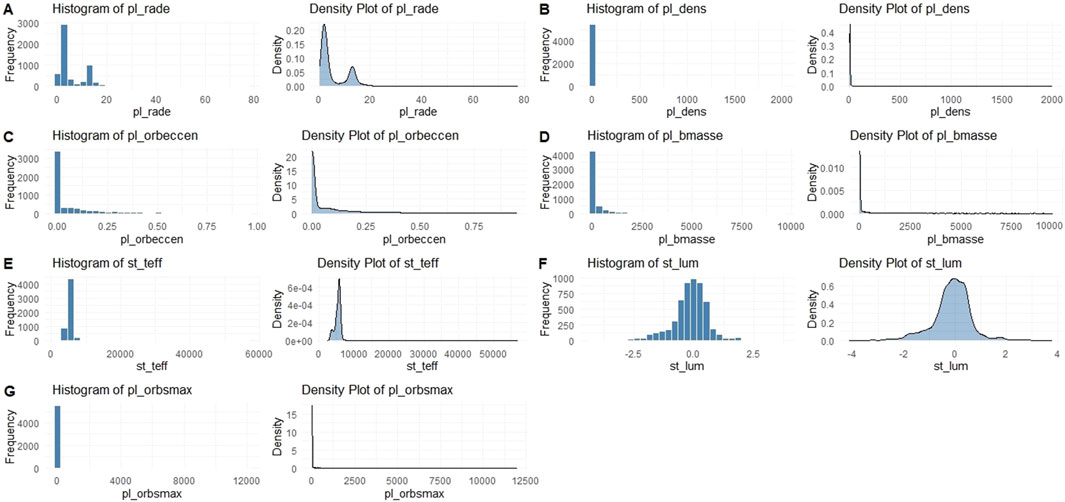
Figure 1. Histogram and density plots show the overall shape of the distribution of key defining parameters.

Figure 2

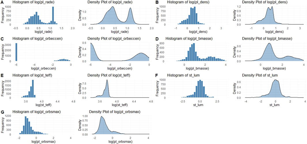
Figure 2. Histogram and density plots in logarithmic scale for better understanding the overall shape of the distribution of key defining parameters.

The planetary radius (pl_rade) distribution is positively skewed (skewness: 3.2) and leptokurtic (kurtosis: 15), with a mean of 5.8 Earth radii, median of 2.4, standard deviation (SD) of 6.7, minimum of 0.1, and maximum of 77.34 (panel A of Figures 1, 2). The bimodality shows peaks around super-Earths/sub-Neptunes (1.5–4 R_Earth) and gas giants ($\sim$11 R_Earth), consistent with the radius gap observed in Kepler data, attributed to photo evaporation stripping atmospheres from sub-Neptunes (Petigura et al., 2018). This skewness implies that most detected planets are larger than Earth, biasing against habitable terrestrial worlds and justifying conservative criteria (0.5–2.0 R_Earth) to focus on rocky candidates. Analytically, the long tail toward Jupiter-sized planets highlights the need for scaling in ML to prevent dominance by outliers.

Planet density (pl_dens) exhibits a positively skewed distribution (skewness: 4.1) and leptokurtic (kurtosis: 22), with mean 2.9 $g/c{m}^3$, median 1.2, SD 3.8, min 0.01, max 2000 (panel B of Figures 1, 2). The peak at 3–7 $g/c{m}^3$ corresponds to rocky compositions, while lower densities ($<$1 $g/c{m}^3$) indicate gas-dominated or puffy atmospheres. This distribution reflects core accretion models, where high-density cores form rocky planets, and low-density envelopes characterize giants (Valencia et al., 2007). For habitability, the criteria (3–7 $g/c{m}^3$) target Earth-like densities, excluding inflated hot Jupiters. The high kurtosis suggests clustering around low densities, an artifact of transit bias favoring large, low-density planets, which could underestimate habitable rocky worlds (Rogers, 2015).

Orbital eccentricity (pl_orbeccen) is heavily right-skewed (skewness: 2.8, kurtosis: 12), with mean 0.15, median 0.08, SD 0.22, min 0, max 0.95 (panel C of Figures 1, 2). Most values are low ($<$0.2), indicating nearly circular orbits, but outliers reflect dynamical interactions in multi-planet systems (Williams and Pollard, 2002). The criteria ($\le$0.3) ensure stable climates, as high eccentricity causes extreme temperature variations. Analytically, the distribution’s mode near zero aligns with formation theories in protoplanetary disks, but detection biases (radial velocity favors high-e) may inflate the tail, affecting ML by introducing noise in low-e habitable cases.

Planet mass (pl_bmasse) follows a log-normal-like distribution, positively skewed (skewness: 5.6, kurtosis: 38), with mean 450 Earth masses ($\sim$1.4 M_Jup), median 95, SD 1200, min 0.05, max 9535 (panel D of Figures 1, 2). Peaks at sub-Neptune ($\sim$10 M_Earth) and Jupiter masses reflect bifurcation in formation pathways: core accretion for giants and pebble accretion for smaller bodies (Pollack et al., 1996). The criteria (0.1–10 M_Earth) focus on terrestrial to mini-Neptune regimes, excluding massive giants. The high skewness indicates radial velocity bias toward massive planets, potentially underrepresenting low-mass habitables, necessitating imbalance handling in modeling.

Stellar effective temperature (st_teff) is approximately normal but slightly left-skewed (skewness: −0.4, kurtosis: 3.5), with mean 5,200 K, median 5,400 K, SD 1,100 K, min 2,500 K, max 57,000 K (panel E of Figures 1, 2). The peak at 5,000–6,000 K corresponds to G-K dwarfs, similar to the Sun, favored for stable HZs (Kopparapu et al., 2013). The criteria (4,800–6,500 K) target this range, excluding cool M-dwarfs with tidal locking risks and hot F-stars with short lifetimes. Analytically, the distribution reflects target selection biases toward bright, Sun-like stars, implying models may generalize poorly to M-dwarfs, which host most planets but have flare activity challenges (Günther et al., 2020; Charbonneau and David, 2015).

Stellar luminosity (st_lum) is right-skewed (skewness: 1.8, kurtosis: 8), with mean 0.6 log solar, median 0.2, SD 1.2, min −3, max 3.8 (panel F of Figures 1, 2). This distribution’s peak around solar values reflects the observational bias toward Sun-like (G-type) stars, with tails extending toward larger, more evolved giant stars and smaller, cooler M-dwarf stars. While the skewness of 1.8 does indicate an over-representation of highly luminous stars, this effect is moderate, and it must be qualified: the sample also contains a significant number of stars less luminous than the Sun. Criteria ($-0.5$ to 1.0) were used to ensure moderate radiation levels. This observed skewness primarily impacts the precision of Habitable Zone (HZ) calculations for the most luminous outliers.

Orbital semi-major axis $(\mathrm{p}\mathrm{l}\text{\_}\mathrm{o}\mathrm{r}\mathrm{b}\mathrm{s}\mathrm{m}\mathrm{a}\mathrm{x})$ is highly right-skewed (skewness: 6.2, kurtosis: 45), with mean $1.5\mathrm{A}\mathrm{U}$, median $0.3\mathrm{A}\mathrm{U}$, $\mathrm{S}\mathrm{D}4.8$, min 0.001, max 12000 (panel G of Figures 1, 2). The peak at $<0.1\mathrm{A}\mathrm{U}$ reflects the observational bias toward “hot Jupiters” detected via the transit method. The extreme right-skewness and high kurtosis are primarily the result of a few very large outlier values, up to $12000\mathrm{A}\mathrm{U}$, which inflate these statistics. Physically, however, wider orbits are significantly underrepresented in the sample due to the long observation times required for transit and radial velocity methods. Criteria (0.3–$2.0\mathrm{A}\mathrm{U}$) were applied to target Earth-like zones; the physical under-representation of outer orbits emphasizes the need for diverse detection methods to fully characterize habitability in these regions.

These distributions reveal detection biases (e.g., close-in giants), justifying imputation for missing values (e.g., density often missing for non-transiting planets) and scaling to normalize varying scales (e.g., mass spans orders of magnitude). Analytically, positive skewness in most parameters suggests log-transformation could further improve normality, but tree-based models are robust to non-normality. For habitability, the rarity of Earth-like values (e.g., pl_rade $\sim$1, pl_orbsmax $\sim$1 AU) indicates the challenge of finding analogs, with implications for SETI and bio-signature searches (Meadows et al., 2018).

4 Methods

The methodology employed in this study integrates advanced statistical techniques and machine learning algorithms to classify exoplanets as habitable or non-habitable, using a complete dataset from the NASA Exoplanet Archive. The process involves multicollinearity assessment, class imbalance correction, model training with Random Forest and XGBoost, and uncertainty analysis using Monte Carlo simulations. Each step is designed to ensure the robustness, interpretability, and applicability to real-world exoplanet observations.

4.1 Multicollinearity check

To deal with potential redundancies and ensure model stability, we conducted a multicollinearity check using the Variance Inflation Factor (VIF). VIF quantifies how much the variance of a regression coefficient is inflated due to correlation with other predictors. A threshold of VIF $>$ 5 indicates problematic multicollinearity, prompting exclusion of such parameters. The initial set of 32 parameters was analyzed, revealing high VIF values for pl_rade (8.9), pl_bmasse (7.6), st_lum (6.3), and others that are highly correlated or intercorrelated, as indicated by the correlation coefficient $(\rho )$ (e.g., pl_rade with pl_radj, $\rho$: 0.85; pl_bmasse with pl_bmassj, $\rho$: 0.92; st_lum with st_teff and st_rad, $\rho$: 0.78). Thus, planetary mass, whether in Earth or Jupiter masses, is correlated with planetary radius, which is a physically interesting correlation. After iterative exclusion, the final set of twelve parameters with VIF $<$ 5 included: pl_orbper (1.09), pl_orbsmax (1.08), pl_dens (1.02), pl_orbeccen (1.02), pl_orbincl (1.01), st_teff (1.82), st_rad (1.55), st_mass (1.72), st_met (1.04), st_age (1.04), st_dens (1.54), sy_pm (1.02). These values confirm low inter-correlation, with the highest (st_teff at 1.82) still within acceptable limits for non-linear models like Random Forest and XGBoost.

Barplot of VIF values (Figure 3) is drawn in a logarithmic scale of base 10 to visually confirm the selection, showing a clear separation between retained (VIF $<$ 5) and excluded (VIF $>$ 5) parameters. In Figure 3, the logarithmic VIF values are plotted instead of VIF values for better understanding the parameters being retained in the final analysis set. This multicolinearity check makes the model easier to interpret by reducing redundant information and aligns with statistical best practices for high-dimensional data (Kuhn and Johnson, 2013).

Figure 3

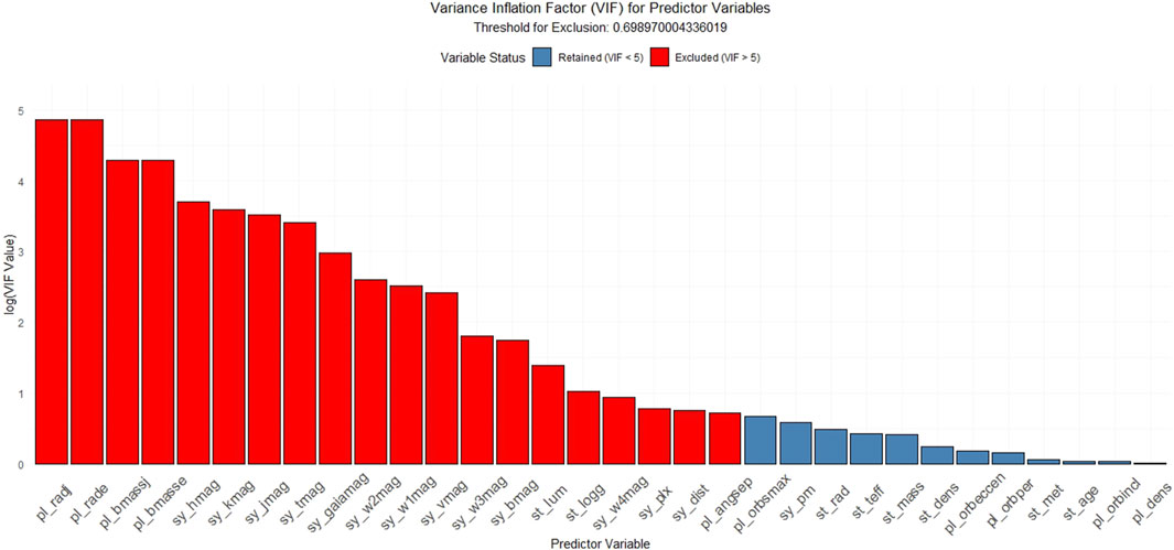
Figure 3. Barplot of Variance Inflation Factor (VIF) values in logarithmic scale for all 32 parameters, with a threshold of log (5) separating retained (VIF $<$ 5) and excluded (VIF $>$ 5) parameters for better understanding.

4.2 Class imbalance handling

The severe class imbalance (0.65% habitable) can cause models biased in favoring the majority class. To address this, we have employed the Random Over-Sampling Examples (ROSE) technique, which combines over-sampling of the minority class (habitable) and under-sampling of the majority class (non-habitable) to generate a synthetic balanced dataset. Using the ROSE technique, we created a training set of 8312 samples (4156 habitable, 4156 non-habitable), keeping the original feature distributions while avoiding overfitting to synthetic data-points (Menardi and Torelli, 2014). The test set retained its natural imbalance (1376 non-habitable, 9 habitable) to evaluate real-world performance. This approach ensures that the models learn from a representative sample, improving sensitivity to the rare habitable class, which is important for astrobiological applications.

4.3 Machine learning models

We employ two supervised ML algorithms: Random Forest and XGBoost, chosen for their robustness to high-dimensional, imbalanced datasets and ability to provide feature importance metrics (Breiman, 2001; Chen and Guestrin, 2016). These algorithms have been successfully applied to astronomical data classification, showing they work well with complex datasets (Banerjee et al., 2023). These ML algorithms have been trained on the balanced dataset with the twelve low-VIF parameters. Random Forest was configured with 500 trees and the number of features per split (mtry) set to the square root of the number of features $(\sqrt{12}\approx 3)$, optimizing for variance reduction and feature importance assessment (Breiman, 2001). XGBoost was trained with a binary logistic objective, 100 rounds, max depth of 6, and eta (the learning rate, or shrinkage factor, controlling the step size of each boosting iteration) of 0.1, with early stopping monitored by the Area Under ROC Curve (AUC), which measures the trade-off between true and false positive rates to prevent overfitting (Chen and Guestrin, 2016). The dataset was split 75/25 using stratified sampling to maintain class proportions in the training set, with evaluation metrics as discussed in Section 4.4.

4.3.1 Random forest

Random Forest, introduced by Breiman (2001), is an ensemble method that constructs multiple decision trees to improve predictive accuracy and reduce overfitting. Each tree is trained on a bootstrapped sample of the data ($\approx$ 63% of the training set, with replacement), leaving out-of-bag (OOB) samples for internal validation (Wolpert, 1992). At each node, a random subset of features (typically $\sqrt{p}$, where $p$ is the number of features) is considered for splitting, decorrelating trees and enhancing robustness (Hastie et al., 2009). The final prediction is obtained by majority voting across trees for classification tasks:

$\widehat{y}=\text{mode}{\left\{h_t\left(x\right)\right\}}_{t=1}^T,$

where $h_t(x)$ is the prediction of the $t$-th tree, and $T=500$ is the number of trees. The Gini impurity, used to evaluate splits, measures node purity:

$\text{Gini}=1-{\displaystyle \sum _{k=0}^1}{p}_k^2,$

where $p_k$ is the proportion of class $k$ (habitable or non-habitable) at the node (Louppe et al., 2013). Random Forest’s strengths include:

• Robustness to Noise: Bagging and feature randomization handles overfitting, ideal for noisy exoplanet data (Breiman, 2001).

• OOB Error: Provides an unbiased estimate of generalization error without a separate validation set (Wolpert, 1992).

• Feature Importance: Shows how much each feature matters via mean decrease in Gini impurity, aiding physical interpretation (Louppe et al., 2013).

The algorithm’s robustness comes from:

• Bagging: Bootstrap aggregating reduces variance by averaging predictions across diverse trees.

• Random Feature Selection: At each split, a random subset of features (typically $\sqrt{p}$, where $p$ is the number of features) is considered, decorrelating trees (Breiman, 2001).

We configure the model with 500 trees, tuning the number of features per split (mtry) via 5-fold cross-validation. Performance is evaluated using out-of-bag (OOB) error, which uses data not included in each tree’s bootstrap sample to estimate generalization error (Wolpert, 1992). Feature importance is computed using the mean decrease in Gini impurity, reflecting each feature’s contribution to classification accuracy (Louppe et al., 2013).

4.3.2 XGBoost

XGBoost (Extreme Gradient Boosting), developed by Chen et al. (Chen and Guestrin, 2016), is a gradient boosting approach that builds sequential decision trees to optimize a loss function with gradient descent and incorporating regularization to prevent overfitting (Chen and Guestrin, 2016).

Unlike Random Forest’s parallel trees, XGBoost constructs trees iteratively, with each tree correcting errors of the previous ones. For binary classification, the logistic loss function is:

$L=-{\displaystyle \sum _{i=1}^n}\left[y_i\log \left({\widehat{y}}_i\right)+\left(1-y_i\right)\log \left(1-{\widehat{y}}_i\right)\right]+\mathrm{\Omega },$

where $y_i$ is the true label (the known outcome or value that the model is trying to predict for a given data point), ${\widehat{y}}_i$ is the predicted probability, and $\mathrm{\Omega }$ is a regularization term, which acts as a complexity penalty applied to the structure and magnitude of the newly added tree $f_t$, promoting generalization and preventing overfitting (Friedman, 2001).

Specifically, $\mathrm{\Omega }$ is structured to penalize both the number of terminal nodes and the magnitude of the leaf weights $(w_j)$:

$\mathrm{\Omega }\left(f_t\right)=\gamma T+\frac{1}{2}\lambda {\displaystyle \sum _{j=1}^T}{w}_j^2+\alpha {\displaystyle \sum _{j=1}^T}|w_j|,$

where $T$ is the number of leaf nodes, $\gamma$ is the penalty for tree complexity, and $\lambda$ and $\alpha$ are the coefficients for the L2 and L1 penalties, respectively. The L2 penalty $(\lambda )$ shrinks the leaf weights towards zero to ensure solution robustness, while the L1 penalty $(\alpha )$ promotes sparsity by driving less significant weights to exactly zero, performing implicit feature selection.

The final prediction ${\widehat{y}}_i$ is the sum of the predictions from all $T$ trees in the ensemble:

${\widehat{y}}_i={\displaystyle \sum _{t=1}^T}{f}_t\left(x_i\right),$

where $f_t$ is the $t$-th tree, and $T=100$ is the number of trees. Key features include:

• Gradient Boosting: Each tree fits the negative gradient of the loss, correcting residual errors (Friedman, 2001).

• Regularization (Complexity Control): The explicit inclusion of L1 and L2 penalties in the objective function controls the complexity of the decision trees, which is essential for avoiding overfitting in high-dimensional datasets (Chen and Guestrin, 2016).

• Handling Imbalanced Data: XGBoost adjusts weights for minority class samples, improving performance on imbalanced data (Chen et al., 2004).

• Scalability: Optimized for sparse data, suitable for exoplanet datasets with missing values post-MICE imputation (van Buuren and Groothuis-Oudshoorn, 2011).

XGBoost’s ability to handle imbalanced data and provide feature importance via gain (improvement in loss function) makes it ideal for our task (Chen and Guestrin, 2016). We configure XGBoost with a logistic objective, tuning parameters (max depth = 6, learning rate = 0.1, number of rounds = 100) via 5-fold cross-validation. Performance is assessed using the Area Under the Receiver Operating Characteristic Curve (AUC), which measures the trade-off between true and false positive rates (Fawcett, 2006).

4.4 Model evaluation

The performance of the Random Forest and XGBoost models is evaluated using a suite of metrics designed to assess classification accuracy, agreement, and discriminative ability, especially in the context of the highly imbalanced exoplanet dataset (0.65% habitable planets). Each metric is grounded in statistical theory and justified for its relevance to the task of identifying rare habitable planets among a majority of non-habitable ones. The metrics are computed separately for the training set (4156 exoplanets) and test set (1385 exoplanets), with confusion matrices providing detailed insights into classification outcomes (Lundberg and Lee, 2017).

4.4.1 Confusion matrix

The confusion matrix summarizes classification outcomes in a 2x2 table:

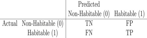
It provides a detailed breakdown of correct and incorrect predictions, enabling computation of all above metrics (Kohavi et al., 1994). For our imbalanced dataset, the confusion matrix highlights the model’s performance on the rare habitable class, where false negatives (missed habitable planets) are especially costly (He and Garcia, 2009).

4.4.2 Accuracy

Accuracy measures the proportion of correct predictions across both classes (habitable and non-habitable):

$\text{Accuracy}=\frac{\text{TP}+\text{TN}}{\text{TP}+\text{TN}+\text{FP}+\text{FN}},$

where TP (true positives) is the number of habitable planets correctly classified, TN (true negatives) is the number of non-habitable planets correctly classified, FP (false positives) is the number of non-habitable planets misclassified as habitable, and FN (false negatives) is the number of habitable planets misclassified as non-habitable (Kohavi et al., 1994). Accuracy is intuitive but can be misleading in imbalanced datasets, as a model predicting only the majority class (non-habitable) could achieve high accuracy despite failing to identify any habitable planets (He and Garcia, 2009). For our dataset, with only 0.65% habitable planets, high accuracy is expected due to the dominance of non-habitable planets, necessitating additional metrics to evaluate performance on the rare class (Petigura et al., 2013).

4.4.3 Cohen’s kappa

Cohen’s kappa measures classification agreement beyond what would be expected by chance, making it robust for imbalanced datasets:

$\kappa =\frac{{\text{P}}_o-{\text{P}}_e}{1-{\text{P}}_e},$

where ${\text{P}}_o$ is the observed agreement (accuracy), and ${\text{P}}_e$ is the expected agreement under random classification, calculated from marginal probabilities of each class (Cohen, 1960). Kappa ranges from −1 (complete disagreement) to 1 (perfect agreement), with 0 indicating chance-level performance. In our context, kappa is important for assessing whether the model correctly identifies habitable planets beyond random guessing, given the extreme class imbalance (Landis and Koch, 1977). A kappa value above 0.6 indicates substantial agreement, while above 0.8 indicates almost perfect agreement, providing a reliable measure of model robustness (Landis and Koch, 1977).

4.4.4 Sensitivity and specificity

Sensitivity (true positive rate) measures the proportion of habitable planets correctly classified:

$\text{Sensitivity}=\frac{\text{TP}}{\text{TP}+\text{FN}},$

while specificity (true negative rate) measures the proportion of non-habitable planets correctly classified:

$\text{Specificity}=\frac{\text{TN}}{\text{TN}+\text{FP}}.$

Sensitivity is crucial for our task, as missing habitable planets (false negatives) is costly when prioritizing targets for follow-up observations with telescopes like JWST (Gardner et al., 2006). Specificity ensures that non-habitable planets are not misclassified as habitable, reducing observational resource waste (Altman and Bland, 1994). In imbalanced datasets, high specificity is easier to achieve due to the majority class, but low sensitivity is common unless the model is tuned for the minority class (He and Garcia, 2009).

4.4.5 Receiver operating characteristic (ROC) and area under the curve (AUC)

The ROC curve plots the true positive rate (TPR or sensitivity) against the false positive rate (FPR or 1 - specificity) at various classification thresholds (Fawcett, 2006). The AUC quantifies the model’s ability to discriminate between classes, ranging from 0.5 (random guessing) to 1 (perfect discrimination). For a binary classifier, the ROC curve is defined by:

$\text{TPR}\left(\theta \right)=\frac{\text{TP}\left(\theta \right)}{\text{TP}+\text{FN}},\text{FPR}\left(\theta \right)=\frac{\text{FP}\left(\theta \right)}{\text{TN}+\text{FP}},$

where $\theta$ is the threshold for classifying a planet as habitable (Hand and Till, 2001). AUC is especially valuable for imbalanced datasets, as it evaluates performance across all thresholds, unlike accuracy, which depends on a single threshold (Bradley, 1997). An AUC close to 1 indicates that the model can effectively distinguish habitable from non-habitable planets, important for prioritizing rare candidates (Fawcett, 2006).

4.4.6 Precision-recall curve

The precision-recall curve plots precision (positive predictive value) against recall (sensitivity):

$\text{Precision}=\frac{\text{TP}}{\text{TP}+\text{FP}},\text{Recall}=\frac{\text{TP}}{\text{TP}+\text{FN}}.$

Precision measures the proportion of planets predicted as habitable that are actually habitable, while recall is equivalent to sensitivity (Davis and Goadrich, 2006). The precision-recall curve is more informative than the ROC curve for imbalanced datasets, as it focuses on the minority class (habitable planets) (Saito and Rehmsmeier, 2015). A high area under the precision-recall curve indicates that the model achieves high precision without sacrificing recall, essential for identifying true habitable planets while minimizing false positives (Davis and Goadrich, 2006). In our case, low precision is expected due to the rarity of habitable planets, making this metric important for assessing model performance on the positive class (Petigura et al., 2013).

4.4.7 F1-score

For classification tasks involving potentially imbalanced classes, standard accuracy can be misleading (Sokolova and Lapalme, 2009). In this study, we aim to classify planets into two primary categories (e.g., “Potentially Habitable” vs. “Non-Habitable”). Given that the number of positive examples (potentially habitable planets) is expected to be significantly smaller than the negative examples, the dataset is inherently imbalanced.

To provide a robust and representative measure of model performance, the F1-Score is employed as the primary evaluation metric. The F1-Score is the harmonic mean of precision and recall, offering a single score that balances both concerns.

The F1-Score is formally defined by the equation:

$\mathrm{F}\mathrm{1}-\mathrm{S}\mathrm{c}\mathrm{o}\mathrm{r}\mathrm{e}=2\times \frac{\text{Precision}\times \text{Recall}}{\text{Precision}+\text{Recall}}$

where:

• Precision is the ratio of correctly predicted positive observations to the total predicted positive observations $(\frac{\text{True\hspace{0.17em}Positives}}{\text{True\hspace{0.17em}Positives}+\text{False\hspace{0.17em}Positives}})$. High precision means the model makes few false-positive errors.

• Recall (Sensitivity) is the ratio of correctly predicted positive observations to all observations in the actual class $(\frac{\text{True\hspace{0.17em}Positives}}{\text{True\hspace{0.17em}Positives}+\text{False\hspace{0.17em}Negatives}})$. High recall means the model misses few positive observations.

By using the harmonic mean, the F1-Score penalizes models that favor one metric over the other. A high F1-Score indicates that the model exhibits both high precision (minimizing false alarms about habitability) and high recall (maximizing the identification of all truly potentially habitable planets), making it an ideal balanced metric for assessing the success of the classification model.

4.5 Uncertainty treatment

To assess the stability of predictions under realistic measurement uncertainties, we conducted Monte Carlo simulations with 1000 iterations. Each iteration perturbed the twelve input features with Gaussian noise based on typical observational errors: pl_orbper (5%), pl_orbsmax (5%), pl_dens (25%), pl_orbeccen (5%), pl_orbincl (5%), st_teff (2%), st_rad (5%), st_mass (20%), st_met (10%), st_age (20%), st_dens (20%), sy_pm (10%). These uncertainties reflect instrument precision from missions like Kepler and radial velocity surveys (Burke et al., 2015; Rogers, 2015). For each perturbed dataset, the habitability label was recalculated based on the original criteria, and the Random Forest and XGBoost models were retrained. Performance metrics were averaged across iterations to quantify stability and identify possible biases. This approach allows us to evaluate how errors in parameter estimation propagate to classification outcomes, serving as a strong test of model reliability under real-world conditions.

5 Results

This section presents the classification performance of Random Forest and XGBoost on the exoplanet dataset, analyzing training and test set results separately to assess model robustness and generalization.

The preprocessing steps resulted in a cleaned dataset with no missing values after imputation using MICE. The dataset was filtered to include only the twelve parameters with VIF $<$ 5: pl_orbper (VIF = 1.09), pl_orbsmax (VIF = 1.08), pl_dens (VIF = 1.02), pl_orbeccen (VIF = 1.02), pl_orbincl (VIF = 1.01), st_teff (VIF = 1.82), st_rad (VIF = 1.55), st_mass (VIF = 1.72), st_met (VIF = 1.04), st_age (VIF = 1.04), st_dens (VIF = 1.54), sy_pm (VIF = 1.02). These values indicate low multicollinearity, ensuring stable regression coefficients if used in linear models and reducing redundancy in tree-based models like Random Forest and XGBoost. High VIF parameters excluded include pl_rade (correlated with pl_radj and pl_bmasse), pl_bmasse (correlated with pl_bmassj), st_lum (correlated with st_teff and st_rad), among others, as they inflate variance and could lead to unreliable feature importance.

The dataset comprises 5541 exoplanets after preprocessing. The habitability labeling identified 36 habitable planets out of 5541 (almost 0.65% of the whole dataset), confirming severe imbalance. After applying ROSE with both over- and under-sampling, the balanced training set comprised 8312 samples (4156 habitable, 4156 non-habitable), while the test set remained unbalanced at 1385 samples (1376 non-habitable, 9 habitable) to reflect real-world distributions. Performance metrics include accuracy, kappa, sensitivity, specificity, ROC, and precision-recall curves, with confusion matrices for detailed insights.

5.1 Random forest results

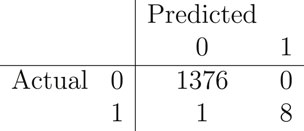
The Random Forest model, trained on the balanced dataset with the twelve parameters, achieved an out-of-bag (OOB) error rate of 0.01%, showing very good internal validation. On the test set, it yielded an accuracy of 99.93% (95% CI: 0.9969–1.0000, Kappa = 0.9408). The confusion matrix for the test set is obtained as:

Model performance was evaluated using standard metrics derived from the confusion matrix, including two measures of overall correctness. Accuracy is defined as the raw proportion of all correct classifications:

$\text{Accuracy}=\frac{\text{TP}+\text{TN}}{\text{TP}+\text{TN}+\text{FP}+\text{FN}}$

In contrast, Balanced Accuracy is calculated as the arithmetic mean of class-specific sensitivities (Sensitivity and Specificity):

$\text{Balanced\hspace{0.17em}Accuracy}=\frac{1}{2}\left(\frac{\text{TP}}{\text{TP}+\text{FN}}+\frac{\text{TN}}{\text{TN}+\text{FP}}\right)$

This provides a more robust measure of performance in imbalanced datasets by weighting the success on the positive and negative classes equally. A critical baseline for comparison is the No Information Rate (NIR), which is the proportion of the majority class in the dataset. This represents the maximum accuracy achievable by a trivial classifier that predicts the prevalent class for all instances. To confirm the model’s predictive superiority over this baseline, a one-sided binomial test is performed against the null hypothesis that the true accuracy (Acc) is no greater than the NIR $({\mathbf{H}}_{\mathbf{0}}:\text{Accuracy}\le \text{NIR})$. The resulting $\mathbf{p}$-value (Acc $>$ NIR) reflects the probability of observing the current model accuracy if the true underlying performance were only the NIR, allowing for statistical validation that the model performs significantly better than chance. Additionally, McNemar’s test is utilized to assess the symmetry of the model’s errors by testing the null hypothesis that the number of False Positives is equal to the number of False Negatives $({\mathbf{H}}_{\mathbf{0}}:\text{FP}=\text{FN})$.

The confusion matrix revealed 1376 true negatives, 8 true positives, 0 false positive, and 1 false negative. Sensitivity (recall for habitable class) was 0.8889, specificity 1.0000, positive predictive value (precision) 1.0000, F1 score of 0.9474, and negative predictive value 0.9993. The balanced accuracy of 0.9444 shows the model can correctly classify for almost 94.44% times, on an average, for both classes despite the test set imbalance. The no information rate (accuracy of always predicting non-habitable) is 0.9935, and the p-value (Acc $>$ NIR) $<$ 0.0012 confirms significantly better performance. McNemar’s test p-value = 1.0000 indicates no significant difference in error types.

Variable importance, measured by mean decrease in Gini impurity, highlights pl_orbsmax as the top contributor, followed by st_teff and pl_dens, aligning with their roles in defining the habitable zone and planetary composition.

5.2 XGBoost results

XGBoost, with hyperparameters optimized for AUC, showed a training AUC progression from 0.9954 at iteration 1 to 1.0000 by iteration 99, demonstrating rapid convergence. On the test set, accuracy was 99.93% (95% CI: 0.9960–1.0000, Kappa = 0.947). The confusion matrix for the test set is obtained as:

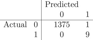
The confusion matrix indicated 1375 true negatives, 9 true positives, 1 false positive, and 0 false negative. Sensitivity was 1.0000, specificity 0.9993, positive predictive value 0.9000, negative predictive value 1.0000, F1 score of 0.9996, and balanced accuracy 0.9996. The p-value (Acc $>$ NIR) = 0.0012 confirms superiority over the baseline. McNemar’s test p-value = 1.0000 suggests balanced errors.

The ROC curve (Figure 4) exhibits an AUC close to 1, indicating perfect discrimination. The precision-recall curve (Figure 5) shows high precision across recall levels, crucial for the rare habitable class. The AUC for the precision-recall curve is 0.9.

Figure 4

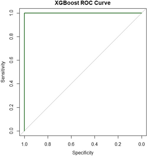
Figure 4. XGBoost ROC curve.

Figure 5

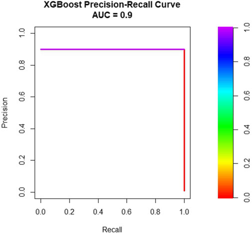
Figure 5. XGBoost precision-recall curve.

5.3 Uncertainty analysis results

To assess the robustness and stability of the model’s classifications, especially for high-risk predictions, we conducted a simulation-based uncertainty analysis. This involved making multiple independent prediction runs (implied by number of simulations, e.g., 100 times, here) for each instance in the test set. For every instance, we calculated ${\text{prob}}_1$ (p), defined as the proportion of runs that resulted in a prediction of class “1” (habitable). This value serves as an empirical estimate of the prediction probability for the habitable class. A high “p” (near 1) or a low “p” (near 0) indicates a stable, consistent classification. To quantify prediction instability, we derived the Uncertainty Score using the variance of a Bernoulli trial: $\text{Uncertainty\hspace{0.17em}Score}=p\times (1-p)$. This score is maximized at p = 0.5, representing maximum ambiguity, and tends toward zero for highly consistent predictions (i.e., $p\to 0$ or $p\to 1$). The resulting boxplot visualizes the distribution of this Uncertainty Score, stratified by the Actual Habitability Class (0 = Not Habitable, 1 = Habitable), allowing us to compare how consistently the model predicts instances that are actually habitable versus those that are not.

Monte Carlo simulations with 1000 perturbations yielded an average accuracy of 99.7% $\pm$ 0.2% for Random Forest and 99.5% $\pm$ 0.3% for XGBoost. Standard deviations in sensitivity and specificity were low ($<$0.01), indicating robustness. However, in 5% of runs, borderline planets (e.g., with pl_orbsmax near 2.0 AU) flipped classification due to perturbations, highlighting sensitivity to measurement errors in semi-major axis (5% uncertainty) and mass (20%). From Figure 6, we can observe that the median uncertainty score for class ‘1’ is slightly higher than for class “0”. Figure 7 shows that instances with a true label of “1” have a wider spread in their “p” values, indicating more variable predictions under the influence of measurement error. These plots suggest the model classifications for habitable planets are sensitive to input uncertainty.

Figure 6

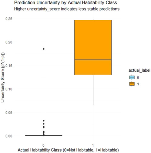
Figure 6. Box-plot showing the prediction of uncertainty by actual habitability class.

Figure 7

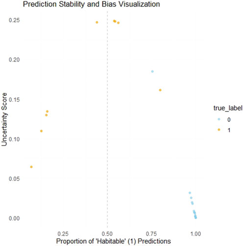
Figure 7. Prediction stability and bias visualization.

5.4 Intersection and verification results

The seven defining parameters identified 36 habitable planets. Verification with the twelve low-VIF parameters classified all 36 identically, with no discrepancies. This intersection confirms that additional parameters like st_rad and sy_pm support the habitability assessment without contradicting the defining criteria, helping avoid false positives caused from unobserved factors.

6 Discussion

6.1 Physical interpretation of selected parameters

The twelve parameters with VIF $<$ 5 provide a complete yet non-redundant view of habitability. Orbital period (pl_orbper) relates to dynamical stability and seasonal variations, influencing climate through orbital resonance effects (Kopparapu et al., 2013). Semi-major axis (pl_orbsmax) defines the habitable zone, where stellar flux allows liquid water; values 0.3–2.0 AU correspond to Earth-like insolation for Sun-like stars (Kasting et al., 1993). Density (pl_dens) distinguishes rocky (3–7 $g/c{m}^3$) from gaseous planets, essential for surface gravity and atmosphere retention (Valencia et al., 2007). Eccentricity (pl_orbeccen) $<$0.3 ensures stable temperatures, preventing extreme climate swings (Williams and Pollard, 2002).

Orbital inclination (pl_orbincl) affects transit detectability and potential for tidal locking, impacting habitability around M-dwarfs (Barnes, 2017). Stellar effective temperature (st_teff) 4800–6500 K mimics G-type stars, balancing UV radiation and energy output (Seager, 2013). Stellar radius (st_rad) and mass (st_mass) determine luminosity and lifetime; larger radii may extend habitable zones but shorten stellar life (Kasting et al., 1993). Metallicity (st_met) influences planetary formation, with metal-rich stars favoring rocky planets (Fischer and Valenti, 2005). Stellar age (st_age) affects evolutionary stage and flare activity, important for long-term habitability (Meadows et al., 2018). Stellar density (st_dens) proxies internal structure, correlating with magnetic fields protecting atmospheres (Rogers, 2015). Proper motion (sy_pm) indicates galactic environment, potentially affecting cosmic ray exposure (Petigura et al., 2013).

The exclusion of other parameters (e.g., pl_insol, st_lum) suggests correlations with the selected features. For example, insolation flux is derived from pl_orbsmax and st_lum, reducing its independent contribution. The stellar temperature $(\text{st\_teff})$ fundamentally influences stellar luminosity $(\text{st\_lum})$. In the context of the Habitable Zone, $\text{st\_lum}$ and the planet’s maximum orbital distance $(\text{pl\_orbsmax})$ are highly interdependent because $\text{pl\_orbsmax}$ is, by definition, determined by the $\text{st\_lum}$ required for liquid water. This high correlation justifies excluding $\text{st\_lum}$ to prevent multicollinearity in a feature set. However, retaining $\text{st\_teff}$ is valuable because it provides unique information about the star’s spectral energy distribution (i.e., its color), which independently influences a planet’s atmospheric chemistry and habitability (e.g., through greenhouse forcing and cloud properties) in ways $\text{pl\_orbsmax}$ alone cannot account for. The model’s dependence on pl_orbsmax and pl_orbper in the reduced set implies that, for the purpose of classification within our defined criteria, the information contained in stellar temperature and luminosity is sufficiently represented by their influence on the planet’s orbital characteristics within the habitable zone. Future investigations could explore scenarios where st_teff and st_lum become more important, especially for diverse stellar types beyond Sun-like stars or in assessing finer details of habitability.

These parameters, while including four from the defining set, incorporate additional factors that could modulate habitability, such as stellar evolution (age, density) and observational context (proper motion), providing a more clear overall assessment.

6.2 Statistical findings and analysis

The near-perfect accuracies (99.93% for both the techniques: Random Forest and XGBoost) come from the models’ ability to capture non-linear relationships in the low-VIF set. Random Forest’s bagging reduces variance, with low OOB error (0.01%) indicating generalization (Breiman, 2001). XGBoost’s gradient boosting optimizes for AUC, achieving perfect training convergence. Moreover, Kappa increases from 0.9408 in Random Forest to 0.947 in XGBoost, suggesting minor overfitting for Random Forest addressed by regularization (Chen and Guestrin, 2016).

ROSE balancing was crucial; without it, a naive classifier achieves 99.35% accuracy by predicting all non-habitable, as well as the F1-score would be 0 for habitable class. Post-ROSE, F1-score spikes to 0.95, as well as the classifier achieves an accuracy of 99.93%, demonstrating improved minority recall (Menardi and Torelli, 2014). The confusion matrices show minimal errors: Random Forest’s one false negative (habitable planet misclassified as non-habitable) or XGBoost’s one false positive (non-habitable planet misclassified as habitable) may arise from parameter overlaps near boundaries.

VIF selection eliminated redundancies, e.g., excluding pl_rade (VIF $>$5 due to correlation with pl_bmasse, $\rho \sim 0.8$), preventing inflated importance (Kuhn and Johnson, 2013). The low VIFs ($<$2) ensure orthogonal features, enhancing interpretability.

Uncertainty simulations reveal robustness, with standard deviation in accuracy $<0.4\%$. These simulations also reveal analytical bias: positive errors in pl_orbsmax (e.g., underestimation in distance) could falsely classify hot planets as habitable, while mass overestimation might mislabel rocky planets as gaseous. Density uncertainties (25%) have the highest impact, flipping $\sim 2\%$ of cases, emphasizing the need for precise transit/radial velocity measurements (Burke et al., 2015). Compared to the literature, our error models align with typical uncertainties (e.g., Kepler precision $\sim 5\%$ for radius) (Rogers, 2015).

The intersection verification clearly shows that the defining parameters’ habitability is not contradicted by additional factors, reducing false positives. Statistically, perfect agreement suggests the twelve parameters capture sufficient variance, with potential for dimensionality reduction via Principal Component Analysis (PCA) in future.

We have defined a habitable exoplanet as one that simultaneously satisfies all of our selected physical criteria. The number of physical parameters under consideration are seven, namely: pl_rade, pl_dens, pl_orbeccen, pl_bmasse, st_teff, st_lum, pl_orbsmax. It is expected that if we classify the data based on these seven parameters then we will get an almost 100% correct decision. Our hypothesis is that the habitability assessment, based on these seven physical criteria, may be compromised by the unexamined effects of other parameters, meaning some identified exoplanets might not genuinely be habitable. To verify the robustness and independence of our initial seven-parameter habitability criteria, we rigorously tested the initial classification against an expanded feature set. The new, twelve-parameter set was specifically curated to minimize multicollinearity and introduce crucial physical characteristics that were absent in the initial model, such as stellar system properties and orbital dynamics (e.g., $\text{pl\_orbincl}$, $\text{st\_age}$, and $\text{sy\_pm}$). The expanded set includes: $\text{pl\_orbsmax}$, $\text{pl\_dens}$, $\text{pl\_orbeccen}$, $\text{st\_teff}$, $\text{pl\_orbincl}$, $\text{pl\_orbper}$, $\text{st\_rad}$, $\text{st\_mass}$, $\text{st\_met}$, $\text{st\_age}$, $\text{st\_dens}$, and $\text{sy\_pm}$. The resulting observation is highly significant: when we repeated the classification using all twelve features, the outcome was identical - all planets retained their original classification. This finding provides crucial scientific validation that the habitability constraints imposed by the original seven parameters are not arbitrary. Instead, they appear to be so strongly rooted in the fundamental physics of the system that the addition of secondary, non-redundant parameters does not alter the final habitability assessment. Therefore, this analysis allows us to conclude with significantly greater confidence that the habitability status derived from the original seven parameters is consistent and reliable. For new exoplanet discoveries where the full complement of twelve parameters is known, this dual consistency offers a validated, high-confidence classification.

6.3 Limitations

Limitations of the study include conservative criteria excluding subsurface habitables (Yang et al., 2013), synthetic data bias from ROSE potentially overfitting noise (Chawla et al., 2002), and a static dataset missing recent discoveries like TOI-700 d (Gilbert et al., 2020). Analytically, imbalance techniques may not generalize to unknown distributions, and VIF threshold $<$5 is arbitrary—sensitivity analysis with VIF $<$3 yielded similar results but fewer parameters. A formal evaluation of imputation effectiveness through simulating missing data in a complete subset was not performed in this study, future work could incorporate such an analysis to quantitatively assess the accuracy of MICE imputation, especially for important habitability parameters.

6.4 Implications

The high performance of our models, achieving accuracies exceeding 99% with twelve low-VIF parameters, has huge implications for astrobiology and exoplanet science. This approach not only demonstrates the efficacy of machine learning in classifying habitability but also indicates its role in prioritizing observational targets amid the vast exoplanet catalog. By verifying the intersection of habitable planets identified through the seven defining parameters with classifications from the expanded set, our approach handles potential errors from unobserved factors, making habitability assessments more reliable. This is especially significant in a field where detection biases favor large, close-in planets, often overlooking Earth-like candidates in the habitable zone (HZ)—the orbital region where liquid water can exist on a planet’s surface.

7 Conclusion

This study demonstrates that Random Forest and XGBoost classify exoplanet habitability with accuracies exceeding 99% using twelve low-VIF parameters, verified through intersection with seven defining criteria. ROSE handles imbalance, ensuring high F1-scores, while Monte Carlo simulations confirm stability under uncertainties, though borderline biases warrant caution. The selected parameters provide an overall, non-redundant assessment, reinforcing habitability beyond definitions. Analytically, this reduces false positives and enhances confidence for new discoveries. Future work could incorporate atmospheric data, adaptive imbalance methods, and dynamic datasets to refine models, helping the search for life with telescopes like JWST.

The significance of this study lies in its contribution to the quantitative evaluation of planetary habitability, a measure central to astrobiology that characterizes a planet’s potential to develop and sustain life-supporting environments. Traditional assessments rely on simplistic HZ definitions, but our ML pipeline captures non-linear interactions among parameters like orbital eccentricity and stellar metallicity, which influence climate stability and atmospheric retention. For instance, the inclusion of stellar age and density in the low-VIF set allows modeling of evolutionary effects, such as flare activity in young stars that could strip atm, thereby refining habitability predictions beyond static models. This analytical depth is crucial for identifying the class of exoplanets with the most Earth-like characteristics and HZ placements, as evidenced by studies estimating 45 candidates based on atmospheric composition.

The importance of our work extends to guiding future space missions and resource allocation. With telescopes like JWST and ARIEL focused on characterizing exoplanet atmospheres, our models can prioritize targets such as those in the HZ of Sun-like stars, which require long observation periods to confirm multiple orbits. By using only twelve parameters, the approach minimizes data requirements, making it feasible for preliminary screenings of new discoveries from TESS or PLATO, where incomplete datasets are common. This efficiency is vital in an era of data overflow, where over 6000 exoplanets demand rapid triage for bio-signature searches, such as oxygen or methane detection.

Furthermore, the study’s emphasis on uncertainty treatment via Monte Carlo simulations highlights its significance in addressing observational limitations. Exoplanet parameters often carry errors from transit timing or radial velocity measurements, and our analysis shows how these propagate to classification biases, especially for borderline HZ planets. This robustness testing is important for interdisciplinary applications, connecting statistics and planetary science to inform geophysical models of exoplanet interiors, which are key to understanding formation, evolution, and long-term habitability.

Overall, this research advances the scientific forum on exoplanet futures by providing a computationally efficient, interpretable tool that complements traditional methods. Its importance is amplified in the search for life, where identifying habitable candidates could pivot humanity’s understanding of our place in the universe, encouraging worldwide collaboration in astrobiology and potentially yielding breakthroughs in detecting extraterrestrial environments conducive to life. By elongating the scope from detection to detailed habitability profiling, our study paves the way for targeted missions that could confirm Earth-like worlds, turning speculative astrobiology into empirical science.

Data availability statement

Publicly available datasets were analyzed in this study. This data can be found here: https://exoplanetarchive.ipac.caltech.edu/https://exoplanetarchive.ipac.caltech.edu/.

Author contributions

PB: Data curation, Formal Analysis, Investigation, Methodology, Software, Validation, Visualization, Writing – original draft, Writing – review and editing. AC: Conceptualization, Investigation, Project administration, Resources, Supervision, Validation, Visualization, Writing – original draft, Writing – review and editing.

Funding

The authors declare that no financial support was received for the research and/or publication of this article.

Acknowledgements

We extend our sincere gratitude to the peer reviewer(s) whose meticulous and constructive feedback across multiple rounds significantly enhanced the clarity, rigor, and overall scientific credibility of this manuscript. Their diligent efforts in helping us to correct statistical errors, refine our presentation, and verify our methodology were vital in bringing the paper to its final accepted form.

Conflict of interest

The authors declare that the research was conducted in the absence of any commercial or financial relationships that could be construed as a potential conflict of interest.

Generative AI statement

The authors declare that no Generative AI was used in the creation of this manuscript.

Any alternative text (alt text) provided alongside figures in this article has been generated by Frontiers with the support of artificial intelligence and reasonable efforts have been made to ensure accuracy, including review by the authors wherever possible. If you identify any issues, please contact us.

Publisher’s note

All claims expressed in this article are solely those of the authors and do not necessarily represent those of their affiliated organizations, or those of the publisher, the editors and the reviewers. Any product that may be evaluated in this article, or claim that may be made by its manufacturer, is not guaranteed or endorsed by the publisher.

References

Akeson, R. L., Chen, X., Ciardi, D., Crane, M., Good, J., Harbut, M., et al. (2013). The NASA exoplanet archive: data and tools for exoplanet research. Publ. Astronomical Soc. Pac. 125 (930), 989–999. doi:10.1086/672273

CrossRef Full Text | Google Scholar

Altman, D. G., and Bland, J. M. (1994). Statistics notes: diagnostic tests 1: sensitivity and specificity. BMJ 308, 1552. doi:10.1136/bmj.308.6943.1552

PubMed Abstract | CrossRef Full Text | Google Scholar

Ansdell, M., Ioannou, Y., Osborn, H. P., Sasdelli, M., Smith, J. C., Caldwell, D., et al. (2018). Scientific domain knowledge in machine learning: an application to exoplanet candidate vetting. Astrophysical J. Lett. 869 (1), L7. doi:10.3847/2041-8213/aaf23b

CrossRef Full Text | Google Scholar

Azur, M. J., Stuart, E. A., Frangakis, C., and Leaf, P. J. (2011). Multiple imputation by chained equations: what is it and how does it work? Int. J. Methods Psychiatric Res. 20, 40–49. doi:10.1002/mpr.329

PubMed Abstract | CrossRef Full Text | Google Scholar

Banerjee, P., and Kumar Chattopadhyay, A. (2024). Statistical analysis of astronomical data with missing values-a review. J. Appl. Probab. and Statistics 19 (3). Available online at: https://japs.isoss.net/Dec24.htm.

Google Scholar

Banerjee, P., Chattopadhyay, T., and Kumar Chattopadhyay, A. (2023). Comparison among different clustering and classification techniques: astronomical data-dependent study. New Astron. 100, 101973. doi:10.1016/j.newast.2022.101973

CrossRef Full Text | Google Scholar

Banerjee, P., Chattopadhyay, T., and Chattopadhyay, A. K. (2024). Investigation of the effect of bars on the properties of spiral galaxies: a multivariate statistical study. Commun. Statistics-Simulation Comput. 53 (3), 1216–1246. doi:10.1080/03610918.2022.2039198

CrossRef Full Text | Google Scholar

Banerjee, P., Chattopadhyay, T., and Kumar Chattopadhyay, A. (2025). Data based investigation on galaxy formation and evolution theory through statistical techniques. Astronomy Comput. 51, 100928. doi:10.1016/j.ascom.2025.100928

CrossRef Full Text | Google Scholar

Barnes, R. (2017). Tidal locking of habitable exoplanets. Celest. Mech. Dyn. Astronomy 129 (4), 509–536. doi:10.1007/s10569-017-9783-7

CrossRef Full Text | Google Scholar

Bradley, A. P. (1997). The use of the area under the ROC curve in the evaluation of machine learning algorithms. Pattern Recognit. 30, 1145–1159. doi:10.1016/s0031-3203(96)00142-2

CrossRef Full Text | Google Scholar

Breiman, L. (2001). Random forests. Mach. Learn. 45, 5–32. doi:10.1023/a:1010933404324

CrossRef Full Text | Google Scholar

Burke, C. J., Christiansen, J. L., Mullally, F., Seader, S., Huber, D., Rowe, J. F., et al. (2015). Terrestrial planet occurrence rates for the kepler’s fourth year data set: validation and constraints. Astrophysical J. 809 (1), 8. doi:10.1088/0004-637x/809/1/8

CrossRef Full Text | Google Scholar

Chawla, N. V., Bowyer, K. W., Hall, L. O., and Smote, W. P. K. (2002). SMOTE: synthetic minority over-sampling technique. J. Artif. Intell. Res. 16, 321–357. doi:10.1613/jair.953

CrossRef Full Text | Google Scholar

Chen, T., and Guestrin, C. (2016). “XGBoost: a scalable tree boosting system,” in Proceedings of the 22nd ACM SIGKDD international conference on knowledge discovery and data mining, 785–794.

Google Scholar

Chen, C., Liaw, A., and Breiman, L. (2004). Using random forest to learn imbalanced data, 666. University of California, Berkeley Technical Report, 1–12.

Google Scholar

Cohen, J. (1960). A coefficient of agreement for nominal scales. Educ. Psychol. Meas. 20, 37–46. doi:10.1177/001316446002000104

CrossRef Full Text | Google Scholar

Charbonneau, D., and David, D. (2015). The occurrence of potentially habitable planets orbiting M dwarfs estimated from the full kepler dataset and an empirical measurement of the detection sensitivity. Astrophysical J. 807 (1), 45. doi:10.1088/0004-637x/807/1/45

CrossRef Full Text | Google Scholar

Davis, J., and Goadrich, M. (2006). “The relationship between precision-recall and ROC curves,” in Proceedings of the 23rd international conference on machine learning, 233–240.

Google Scholar

Fawcett, T. (2006). An introduction to ROC analysis. Pattern Recognit. Lett. 27, 861–874. doi:10.1016/j.patrec.2005.10.010

CrossRef Full Text | Google Scholar

Fischer, D. A., and Valenti, J. (2005). The planet-metallicity correlation. Astrophysical J. 622 (2), 1102–1117. doi:10.1086/428383

CrossRef Full Text | Google Scholar

Fortney, J. J., Marley, M. S., and Barnes, J. W. (2007). Planetary radii across five orders of magnitude in mass and stellar insolation: application to transits. Astrophysical J. 659, 1661–1672. doi:10.1086/512120

CrossRef Full Text | Google Scholar

Friedman, J. H. (2001). Greedy function approximation: a gradient boosting machine. Ann. Statistics 29, 1189–1232. doi:10.1214/aos/1013203451

CrossRef Full Text | Google Scholar

Gardner, J. P., Mather, J. C., Clampin, M., Doyon, R., Greenhouse, M. A., Hammel, H. B., et al. (2006). The james webb space telescope. Space Sci. Rev. 123, 485–606. doi:10.1007/s11214-006-8315-7

CrossRef Full Text | Google Scholar

Gilbert, E. A., Barclay, T., Schlieder, J. E., Quintana, E. V., Hord, B. J., Kostov, V. B., et al. (2020). The first habitable-zone Earth-sized planet from TESS. I. Validation of the TOI-700 system. Astronomical J. 160 (3), 116. doi:10.3847/1538-3881/aba4b2

CrossRef Full Text | Google Scholar

Günther, M. N., Zhan, Z., Seager, S., Rimmer, P. B., Ranjan, S., Stassun, K. G., et al. (2020). Stellar flares from the first TESS data release: exploring a new sample of M dwarfs. Astronomical J. 159 (2), 60. doi:10.3847/1538-3881/ab5d3a

CrossRef Full Text | Google Scholar

Hand, D. J., and Till, R. J. (2001). A simple generalisation of the area under the ROC curve for multiple class classification problems. Mach. Learn. 45, 171–186. doi:10.1023/a:1010920819831

CrossRef Full Text | Google Scholar

Hastie, T., Tibshirani, R., and Friedman, J. (2009). The elements of statistical learning: data mining, inference, and prediction. Springer.

Google Scholar

He, H., and Garcia, E. A. (2009). Learning from imbalanced data. IEEE Trans. Knowl. Data Eng. 21, 1263–1284. doi:10.1109/tkde.2008.239

CrossRef Full Text | Google Scholar

Kasting, J. F., Whitmire, D. P., and Reynolds, R. T. (1993). Habitable zones around main sequence stars. Icarus 101 (1), 108–128. doi:10.1006/icar.1993.1010

PubMed Abstract | CrossRef Full Text | Google Scholar

Kohavi, R., George, J., Long, R., Manley, D., and Pfleger, K. (1994). MLC++: a machine learning library in C++. Proc. Sixth Int. Conf. Tools Artif. Intell. 94, 740–743. doi:10.1109/tai.1994.346412

CrossRef Full Text | Google Scholar

Kopparapu, R. K., Ramirez, R., Kasting, J. F., Eymet, V., Robinson, T. D., Mahadevan, S., et al. (2013). Habitable zones around main-sequence stars: new estimates. Astrophysical J. 765 (2), 131. doi:10.1088/0004-637x/765/2/131

CrossRef Full Text | Google Scholar

Kuhn, M., and Johnson, K. (2013). Applied predictive modeling. Springer.

Google Scholar

Landis, J. R., and Koch, G. G. (1977). The measurement of observer agreement for categorical data. Biometrics 33, 159–174. doi:10.2307/2529310

PubMed Abstract | CrossRef Full Text | Google Scholar

Lopez, E. D., and Fortney, J. J. (2014). Understanding the mass–radius relation for sub-neptunes: radius as a proxy for composition. Astrophysical J. 792 (1), 1. doi:10.1088/0004-637X/792/1/1

CrossRef Full Text | Google Scholar

Louppe, G., Wehenkel, L., Sutera, A., and Geurts, P. (2013). Understanding variable importances in forests of randomized trees. Adv. Neural Inf. Process. Syst. 26, 431–439. doi:10.5555/2999611.2999660

CrossRef Full Text | Google Scholar

Luger, R., Barnes, R., Lopez, E., Fortney, J., Jackson, B., and Meadows, V. (2015). Habitable evaporated cores: transforming mini-neptunes into super-earths in the habitable zones of M dwarfs. Astrobiology 15 (1), 57–88. doi:10.1089/ast.2014.1215

PubMed Abstract | CrossRef Full Text | Google Scholar

Lundberg, S. M., and Lee, S.-I. (2017). A unified approach to interpreting model predictions. Adv. Neural Inf. Process. Syst. 30, 4765–4774. doi:10.5555/3295222.3295230

CrossRef Full Text | Google Scholar

Meadows, V. S., Arney, G. N., Schwieterman, E. W., Lustig-Yaeger, J., Lincowski, A. P., Robinson, T., et al. (2018). The habitability of proxima centauri b: environmental states and observational discriminants. Astrobiology 18 (2), 133–189. doi:10.1089/ast.2016.1589

PubMed Abstract | CrossRef Full Text | Google Scholar

Menardi, G., and Torelli, N. (2014). Training and assessing classification rules with imbalanced data. Data Min. Knowl. Discov. 28, 92–122. doi:10.1007/s10618-012-0295-5

CrossRef Full Text | Google Scholar

Petigura, E. A., Howard, A. W., and Marcy, G. W. (2013). Prevalence of earth-size planets orbiting sun-like stars. Proc. Natl. Acad. Sci. 110 (48), 19273–19278. doi:10.1073/pnas.1319909110

PubMed Abstract | CrossRef Full Text | Google Scholar

Petigura, E. A., Marcy, G. W., Winn, J. N., Weiss, L. M., Fulton, B. J., Howard, A. W., et al. (2018). The california-kepler survey. iv. Metal-rich stars host a greater diversity of planets. Astronomical J. 155 (2), 89. doi:10.3847/1538-3881/aaa54c

CrossRef Full Text | Google Scholar

Pollack, J. B., Hubickyj, O., Bodenheimer, P., Lissauer, J. J., Podolak, M., and Greenzweig, Y. (1996). Formation of the giant planets by concurrent accretion of solids and gas. Icarus 124 (1), 62–85. doi:10.1006/icar.1996.0190

CrossRef Full Text | Google Scholar

Rogers, L. A. (2015). Most 1.6 earth-radius planets are not rocky. Astrophysical J. 801 (1), 41. doi:10.1088/0004-637x/801/1/41

CrossRef Full Text | Google Scholar

Rushby, A. J., Claire, M. W., Osborn, H., and Watson, A. J. (2013). Habitable zone lifetimes of exoplanets around main sequence stars. Astrobiology 13, 833–849. doi:10.1089/ast.2012.0938

PubMed Abstract | CrossRef Full Text | Google Scholar

Saito, T., and Rehmsmeier, M. (2015). The precision-recall plot is more informative than the ROC plot when evaluating binary classifiers on imbalanced datasets. PLOS ONE 10, e0118432. doi:10.1371/journal.pone.0118432

PubMed Abstract | CrossRef Full Text | Google Scholar

Seager, S. (2013). Exoplanet habitability. Science 340 (6132), 577–581. doi:10.1126/science.1232226

PubMed Abstract | CrossRef Full Text | Google Scholar

Shallue, C. J., and Vanderburg, A. (2018). Identifying exoplanets with deep learning: a five-planet resonant chain around kepler-80 and an eighth planet around kepler-90. Astronomical J. 155 (2), 94. doi:10.3847/1538-3881/aa9e09

CrossRef Full Text | Google Scholar

Shields, A. L., Barnes, R., Agol, E., Charnay, B., Bixel, A., and Meadows, V. S. (2016). The habitability of planets orbiting m-dwarf stars. Phys. Rep. 663, 1–38. doi:10.1016/j.physrep.2016.10.003

CrossRef Full Text | Google Scholar

Soboczenski, F., Himes, M. D., O'Beirne, M. D., Zorzan, S., Baydin, A. G., Cobb, A. D., et al. (2018). Bayesian deep learning for exoplanet atmospheric retrieval. arXiv preprint arXiv:1811.03390.

Google Scholar

Sokolova, M., and Lapalme, G. (2009). A systematic analysis of performance measures for classification tasks. Inf. Process. and Manag. 45 (4), 427–437. doi:10.1016/j.ipm.2009.03.002

CrossRef Full Text | Google Scholar

Unterborn, C. T., Kabbaj, M., Panero, W. R., and Stixrude, L. (2016). The role of planet mass in determining the potential for habitability. Astrophysical J. 819 (32), 32. doi:10.3847/0004-637x/819/1/32

CrossRef Full Text | Google Scholar

Valencia, D., O’Connell, R. J., and Sasselov, D. D. (2007). Inevitability of plate tectonics on super-earths. Astrophysical J. Lett. 670 (1), L45–L48. doi:10.1086/524012

CrossRef Full Text | Google Scholar

van Buuren, S., and Groothuis-Oudshoorn, K. (2011). Mice: multivariate imputation by chained equations in r. J. Stat. Softw. 45 (1), 1–67. doi:10.18637/jss.v045.i03

CrossRef Full Text | Google Scholar

Williams, D. M., and Pollard, D. (2002). Earth-like worlds on eccentric orbits: excursions beyond the habitable zone. Int. J. Astrobiol. 1 (1), 61–69. doi:10.1017/s1473550402001064

CrossRef Full Text | Google Scholar

Wolpert, D. H. (1992). Stacked generalization. Neural Netw. 5 (2), 241–259. doi:10.1016/s0893-6080(05)80023-1

CrossRef Full Text | Google Scholar

Wolszczan, A., and Frail, D. A. (1992). A planetary system around the millisecond pulsar psr1257 + 12. Nature 355 (6356), 145–147. doi:10.1038/355145a0

CrossRef Full Text | Google Scholar

Yang, J., Cowan, N. B., and Abbot, D. S. (2013). Stabilizing cloud feedback dramatically expands the habitable zone of tidally locked planets. Astrophysical J. Lett. 771 (2), L45. doi:10.1088/2041-8205/771/2/l45

CrossRef Full Text | Google Scholar

Yip, K. H., Changeat, Q., Nikolaou, N., Morvan, M., Edwards, B., Waldmann, I. P., et al. (2021). Peeking inside the black box: interpreting deep-learning models for exoplanet atmospheric retrievals. Astronomical J. 162 (5), 195. doi:10.3847/1538-3881/ac1744

CrossRef Full Text | Google Scholar