Abstract
Vehicle speed and axle spacing are key parameters that shape the pavement vibration response and serve as essential prior inputs for downstream models such as axle-load estimation and hidden-void detection. Obtaining them from external systems such as video is vulnerable to weather and to time-synchronisation errors between systems, whereas estimating them from the pavement vibration signal itself enables closed-loop interpretation of traffic information and structural state within a single embedded system. Using field data from embedded MEMS accelerometers, this study reconstructs the signal with complete ensemble empirical mode decomposition with adaptive noise (CEEMDAN) and dominant-frequency screening, builds an instantaneous total-energy curve via the continuous wavelet transform, and estimates speed and axle spacing by pairing prominent energy peaks across two sensors; the method is compared, under identical criteria, with a time-domain envelope peak method. For 12 field passes of a four-axle truck (25.00–55.62 t, 40–60 km/h), both methods succeed in every case. Over the ten cases evaluated against the 7750 mm total wheelbase, the two methods have similar median errors (6.5% vs. 6.8%), whereas the wavelet energy method has a lower mean (6.2% vs. 8.8%), a narrower interquartile range (3.3 vs. 4.8 percentage points) and a much lower maximum (10.5% vs. 33.8%); in the two cases evaluated against the 1350 mm rear-axle spacing the errors are 2.8%–3.9% and 3.2%–4.5%. The energy method was more stable under noise spikes (6.5% vs. 33.8% in the same case), insensitive to the frequency band and to the wavelet scale grid, and required no case-dependent parameter tuning, whereas the envelope method depends on a window length whose optimum drifts with speed. The reconstructed signal also preserves waveform and spectral information, providing a reusable time-frequency feature for downstream models.
1 Introduction
The intelligence of transportation infrastructure has become an important trend in highway development (Yang et al., 2023; Du et al., 2022). A key prerequisite for intelligent road operation is the continuous and accurate perception of pavement condition and traffic state. In this respect, pavement dynamic-response monitoring directly captures the real-time internal response of the pavement structure under vehicle loading; it not only helps characterise how pavement performance evolves under the coupled effects of traffic load and environment, but also provides a data basis for retrieving traffic information such as vehicle speed, axle spacing, vehicle type, and axle load. Vehicle-road integrated perception based on pavement dynamic response is therefore an important technical route for supporting smart roads, structural health monitoring, and refined maintenance.
Existing vehicle-road perception techniques fall into two broad categories: non-intrusive and embedded sensing. Non-intrusive techniques, such as cameras (; ) and lidar (Sánchez-Oro et al., 2013), are relatively easy to deploy and offer wide coverage, but are sensitive to illumination, occlusion, human factors, and adverse weather, which degrade data stability and recognition accuracy. They also generate large volumes of video or point-cloud data, leading to high transmission and processing costs (). More importantly, an external traffic-sensing system and the internal pavement-response monitoring usually belong to two separate systems, and the time-synchronisation error between them limits any joint interpretation of traffic information and pavement dynamic-response data. Remote sensing can provide wide-area traffic information but is limited in single-vehicle accuracy and in acquiring the key internal pavement response ().
Embedded monitoring, by contrast, can be installed directly inside or just beneath the pavement structure and thus captures the true structural response under vehicle loading. Weigh-in-motion systems are already widely used for traffic-load monitoring, but their energy consumption and construction and maintenance costs are high, making dense, large-scale deployment difficult, and they mainly serve traffic-information monitoring (Zhang et al., 2015; ; Sujon and Dai, 2021). A range of embedded approaches—fibre Bragg grating and distributed optical-fibre sensing (Wang HP. et al., 2020; Tan et al., 2008; ), MEMS accelerometers (Sabato et al., 2016; ), wireless sensor networks and IoT-based monitoring (Ye et al., 2018a; ; Ye et al., 2024; Ye, 2019), embedded stress-strain sensing (; ; ), and roadside sensing ()—have been used to acquire the pavement dynamic response under vehicle loading and to support structural-state analysis and traffic-information extraction; combined with data-driven methods such as physics-informed neural networks, the monitoring data can further be used to invert pavement material parameters, broadening the application scope of embedded monitoring (Xing et al., 2026). In recent years, advances in micro-electro-mechanical systems (MEMS) have steadily improved the sensitivity, frequency response, physical size, and power consumption of MEMS sensors, which now offer low cost, low power, miniaturisation, high integration, and easy scalability, together with the potential for edge computing and wireless communication (; ). Pavement-vibration monitoring with MEMS accelerometers therefore offers the prospect of acquiring traffic information and sensing structural state in a coordinated way within a single embedded system. Table 1 summarises the key aspects of these sensing technologies: how they are deployed, how they respond to weather and illumination, whether they share a time base with the pavement response, and what information they provide.
TABLE 1
| Technology | References | Category | Sensitivity to weather and illumination | Same time base as the pavement response | Information provided |
|---|---|---|---|---|---|
| Camera/video | (; ) | Non-intrusive, roadside | High (illumination, occlusion, adverse weather) | No, separate system | Vehicle type, speed, trajectory; large video streams |
| Lidar/radar | (Sánchez-Oro et al., 2013) | Non-intrusive, roadside | Lidar affected by adverse weather; large point-cloud data | No, separate system | Vehicle position, speed |
| Remote sensing | () | Satellite or airborne | Depends on acquisition conditions; limited single-vehicle accuracy | No | Wide-area traffic information |
| Weigh-in-motion | (Zhang et al., 2015; ; Sujon and Dai, 2021) | Embedded | Low (in-pavement sensors); high energy and maintenance cost | Own system; not designed for structural response | Axle load, speed, axle spacing |
| Fibre Bragg grating/distributed fibre | (Wang et al., 2020a; Tan et al., 2008; ) | Embedded | Low; temperature affects readings | Yes | Strain and temperature response of the pavement |
| Strain and stress sensors | (; ; ) | Embedded | Low; temperature affects readings | Yes | Pavement moduli, traffic loads |
| Roadside sensors | (; ) | Non-intrusive, roadside | Moderate | No | Vehicle classification, speed |
| MEMS accelerometers (this study) | (Sabato et al., 2016; ; ; ) | Embedded | Not affected by illumination or precipitation; temperature changes the response amplitude | Yes | Vibration response; speed and axle spacing (this study), axle load and structural state (downstream) |
Comparison of vehicle-road perception technologies discussed in this section.
Previous studies have shown that deploying vibration sensors in asphalt-concrete pavement enables real-time monitoring of traffic information such as vehicle speed, axle spacing, and load position (Ye, 2019; ; Zeng et al., 2020; Wang H. et al., 2020; ; Ye et al., 2020; Shi et al., 2021). These studies confirm the feasibility of extracting traffic information from pavement vibration signals and provide a technical basis for response-based vehicle-road perception. Speed and axle spacing are not only important traffic parameters but also key prior variables for interpreting the pavement dynamic response. The vibration induced by vehicle load is affected by many factors, including axle load, axle configuration, speed, and ambient temperature (); to address the randomness of the load parameters, stochastic vibration analyses of pavement systems have been carried out, supporting load-response modelling (). Among these factors, axle configuration and axle spacing determine the number and spacing of the response peaks; speed determines the peak time intervals and also changes the vibration amplitude and the frequency distribution. As speed increases, the primary and secondary frequency ranges of the signal shift towards higher frequencies. Vibration amplitude and dominant frequency are, in turn, important indicators of structural damage, stiffness degradation and local anomalies (Wang H. et al., 2020; ; Ye et al., 2020); unless the influence of speed and axle spacing is separated first, these indicators cannot be interpreted reliably. Accurate estimation of speed and axle spacing therefore serves two purposes in pavement-vibration-based monitoring: it provides traffic information, and it is a prerequisite for axle-load estimation, load identification and hidden-distress diagnosis.
At present, most speed- and wheelbase-estimation methods identify the local peak generated as a vehicle passes over a sensor and compute the result from the peak time difference between two sensors of known spacing (Ye, 2019; Shi et al., 2021; ; Ye et al., 2018b). Such methods are intuitive and easy to implement, but rely heavily on time-domain peak detection. Under low signal-to-noise ratio, weak front-axle response, large lateral offset between wheel path and sensor, or markedly different response strengths among axle groups, axle peaks are prone to being missed, falsely detected, or mismatched, which increases the estimation error. Moreover, the pavement vibration response is strongly non-stationary and multi-scale; the response from different axle groups is affected by the layered structure of the pavement, sensor embedment depth, lateral wheel-path offset, and ambient noise, so a time-domain peak does not always correspond reliably to the true instant of axle loading. Relying on time-domain peaks alone also discards frequency, phase, and energy-distribution information, making it hard to fully exploit how the vibration energy evolves in the time-frequency domain during a vehicle pass. Existing studies therefore still discuss the basis for selecting peak-extraction parameters, the cross-condition robustness, and the recoverability under weak-axle-peak conditions only insufficiently. There is a need for a more robust speed- and wheelbase-estimation method built from a time-frequency energy perspective, to overcome the limitations of conventional peak detection under complex conditions.
Empirical mode decomposition (EMD) and its variants are important tools for processing nonlinear, non-stationary signals (Rilling et al., 2003; Tang et al., 2011; ; Wu and Huang, 2009). Among them, complete ensemble empirical mode decomposition with adaptive noise (CEEMDAN), developed from EMD, introduces adaptive noise and performs a complete ensemble average, which alleviates residual noise and mode mixing while retaining the local time-frequency features of the signal; it has been applied in engineering vibration analysis such as bearing-fault diagnosis () and bridge health monitoring (). Because pavement vibration signals are clearly non-stationary, multi-scale, and noise-sensitive, CEEMDAN provides a suitable basis for the multi-scale decomposition and effective-component reconstruction of pavement vibration under vehicle loading. However, for asphalt-pavement vibration signals, studies that combine CEEMDAN reconstruction with continuous wavelet time-frequency energy analysis and further use it to assess speed- and wheelbase-estimation accuracy remain relatively scarce.
Based on the above analysis, this paper uses field loading data collected by an embedded asphalt-pavement vibration monitoring system, builds the instantaneous total-energy curve of the vibration signal with CEEMDAN and the continuous wavelet transform, proposes a speed- and wheelbase-estimation method based on prominent energy peaks, and compares it systematically with the time-domain envelope peak method. The main contributions are as follows. (1) A speed- and wheelbase-estimation method of the form “CEEMDAN reconstruction - wavelet instantaneous total energy - cross-sensor pairing of prominent energy peaks” is proposed; it uses the objectively known true wheelbase as the accuracy reference and ensures recoverability under weak-axle-peak conditions through a transit-time self-consistency check and a rear-axle-pair fallback criterion. (2) A same-criterion comparison with the time-domain envelope peak method over 12 field cases shows that both methods succeed in every case and have similar median errors, but that the energy method has a lower mean error (6.2% vs. 8.8% over the ten total-wheelbase cases) and a lower error bound (10.5% vs. 33.8%), is more robust to noise spikes, depends less on parameter choice, and preserves more of the signal information. (3) The resulting instantaneous time-frequency energy distribution provides a reusable feature representation for downstream tasks such as axle-load estimation, laying a foundation for closed-loop interpretation of traffic information and structural state within a single embedded system.
The remainder of this paper is organised as follows. Section 2 describes the field loading test and pavement-vibration data acquisition; Section 3 presents the vibration-signal reconstruction based on CEEMDAN decomposition with dominant-frequency and energy screening; Section 4 proposes the speed- and wheelbase-estimation method based on the wavelet instantaneous total-energy peaks and compares it with the envelope peak method over the 12 field cases, and analyses the uncertainty, parameter sensitivity and applicability range of the method; Section 5 concludes the paper.
2 Field vibration test and data acquisition
2.1 Test section and sensor layout
A field loading test was carried out on an asphalt pavement in Zhaotong, Yunnan Province, China. From top to bottom, the pavement structure of the test section consists of an AC-13 surface course (4 cm), an AC-20 binder course (6 cm), an AC-25 base course (8 cm), a cement-stabilised macadam base (36 cm), a lime-and-fly-ash-stabilised macadam subbase (18 cm), and the subgrade.
The accelerometers were embedded inside the asphalt pavement during paving. After the binder course was completed, slots were cut in it with a groove cutter according to the sensor dimensions; the bottom of each slot was first filled with emulsified asphalt and asphalt mortar, the sensor was placed horizontally in the slot, emulsified asphalt and asphalt mortar were then injected into the gap between the sensor and the slot, and the gap was tapped with a rubber hammer to fix the sensor. The sensor area was then covered with surface-course asphalt about 1–2 cm thick, the sensor and lead-wire area was compacted with a small compactor, and the surface was finally paved. In this test, two accelerometers were embedded beneath the wheel path of the driving lane, one behind the other along the driving direction, 2.5 m apart and at a depth of 4 cm. Figure 1 is a top view of the measurement section: it shows their position relative to the lane and to the wheel paths of the test truck, together with the roadside gateway and the cloud platform of the monitoring system.
FIGURE 1
The accelerometer sampling frequency was set to = 1000 Hz. By the sampling theorem (Shannon, 1949), the Nyquist frequency = 500 Hz is the highest frequency that can be represented without aliasing. The measured spectra (Section 3.1; Figure 2) show that the vehicle-related modes have dominant frequencies below 200 Hz and that the highest-frequency mode (IMF1, about 370 Hz) is broadband tyre-pavement noise; the sampling frequency therefore satisfies with a margin of more than a factor of two for the 2–200 Hz band used in the estimation, and it provides the 1 ms time resolution of the peak-time differences whose effect on the estimates is quantified in Section 4.4. The pavement-vibration acceleration signals generated as a vehicle passes are transmitted in real time to a roadside gateway over a cable, and then uploaded to a cloud platform over a wireless network.
FIGURE 2
2.2 Test cases
A four-axle truck with a wheelbase of 7750 mm (axle spacings of 2100 + 4300 + 1350 mm) was used. The two front axles are single-tire steering axles, and the two rear axles are dual-tire driving axles (two tires on each side of each axle). The test was conducted in the main lane at the monitoring section: the truck passed the measurement point at gross weights of 25.00, 34.98, 45.39, and 55.62 t, each at about 40, 50, and 60 km/h, giving 12“weight x speed” cases in total. Vehicle information and the test cases are listed in Table 2. Two traffic cones were placed on the section, with a spacing matched to the vehicle track width, to guide the truck through their centre so that the tires accurately struck the embedded sensor positions, thereby standardising the driving path and reducing the effect of lateral offset on the vibration data.
TABLE 2
| Item | Value |
|---|---|
| Vehicle type | Heavy dump truck CA3310P66K24L6T4AE5 |
| Axle configuration | Four axles: two single-tyre steering axles (axles 1 and 2) and two dual-tyre driving axles (axles 3 and 4) |
| Axle spacings | 2100 mm (axles 1–2), 4300 mm (axles 2–3), 1350 mm (axles 3–4); total wheelbase 7750 mm |
| Gross weight | 25.00, 34.98, 45.39 and 55.62 t |
| Nominal speed | 40, 50 and 60 km/h |
| Appearance | 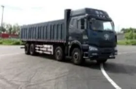 |
Information on the test vehicle.
During the test, one person drove the vehicle while another in the passenger seat recorded the nominal speed at the cone position. Because of manual reading and driving fluctuation, the recorded speed deviates somewhat from the true speed; in the following analysis the speed is further estimated from the pavement vibration signal and cross-checked.
2.3 Pavement vibration data
2.3.1 Pavement vibration response at different speeds
Figure 3 shows the time- and frequency-domain curves for the 25 t four-axle truck at 40, 50, and 60 km/h.
FIGURE 3
For the four-axle truck, the time-domain plot clearly reflects the acceleration change as each axle passes, forming four distinct peaks and troughs. As speed increases, the peak and trough amplitudes grow, and the spacing between peaks is closely related to speed: at low speed (e.g., 40 km/h) the inter-axle passage time is longer and the peaks are more widely spaced, whereas at high speed (e.g., 60 km/h) the passage time shortens and the peaks become closer. The dominant-frequency amplitude in the frequency domain also increases with speed; affected by the real pavement condition and ambient noise, the signal also contains high-frequency and random components.
2.3.2 Pavement vibration response under different loads
Figure 4 shows the time- and frequency-domain curves at a fixed speed of 40 km/h for gross weights of 25.00, 34.98, and 55.62 t.
FIGURE 4
As shown by the time-domain signals in Figure 4, the vibration amplitude increases markedly with vehicle weight: the peak-to-peak amplitude rises from about 50 mg for the 25.00 t truck to about 74 mg and 83 mg for the 34.98 t and 55.62 t trucks, directly reflecting the effect of the total vehicle weight on the pavement dynamic response. In the frequency domain, the amplitudes of both heavier vehicles are clearly higher than that of the 25.00 t truck, while for all three weights the vibration energy remains concentrated in the low-frequency band.
3 Reconstruction of pavement vibration signals
3.1 Empirical mode decomposition of the vibration signal
To further characterise the pavement vibration at different speeds, the improved EMD method CEEMDAN is used to analyse the signals captured by the accelerometers. Building on EMD, CEEMDAN adds a series of white-noise realisations to enhance the local features of the signal and make it easier to decompose and analyse (
). White noise is a fully random signal with a uniform power spectral density across all frequencies; by setting the number of noise realisations and their standard deviation, the amount and strength of the added noise can be controlled. The main steps are as follows.
Normalise the original signal (Equation 1):
where
is the standard deviation of the original signal.
2. Generate a set of white-noise realisations and apply EMD to each to obtain the noise modal components.
3. Add the noise to the original signal (Equation 2):
and apply EMD to each realisation to extract the first mode; the first modal component is then averaged as (
Equation 3):
4. Compute the remaining modes iteratively. At the kth iteration, the first k-1 modes are removed from the signal to obtain the residual, as in Equation 4:
5. For the residual, the first-mode extraction procedure is repeated using the corresponding noise modes. For each noise realisation, if it contains the k-th noise mode, that mode is first normalised, scaled by the standard deviation, and added to the residual; the components from Equation 3 are accumulated and averaged. EMD is then applied to the modified signal to extract its mode. This is repeated for every noise realisation, giving a new modal component for each, and the process continues until the residual can no longer be decomposed.
6. The normalised signal is reconstructed by summing all modes (Equation 5):
and the reconstructed signal is then de-normalised (
Equation 6):
Through this iterative process, CEEMDAN progressively extracts all significant frequency components, each step capturing the most dominant oscillation not yet extracted. The number of noise realisations is set to 200 and the noise standard deviation to 0.2, following established practice for noise-assisted decomposition (Wu and Huang, 2009; ; ; Yeh et al., 2010). The maximum number of sifting iterations per mode is 1000 (the default of the PyEMD implementation, version 1.9.0). The sensitivity of the estimates to the number of realisations and to the noise standard deviation is examined in Section 4.4.
Figure 2 shows the decomposition result for the 25 t four-axle truck at 60 km/h, together with the spectral analysis of the individual modes.
Ten modes are obtained from the decomposition. IMF1 is a high-frequency component with a dominant frequency of about 370 Hz, arising mainly from the high-frequency impact and broadband noise excited at the tire-pavement contact; although related to vehicle passage, it is sharp and fragmented in time. IMF2-IMF7 have dominant frequencies between 2 and 200 Hz and show clear non-stationary transients that are strongly correlated with the vibration induced by vehicle passage. IMF8-IMF10 are low-frequency components with substantial amplitude near 0 Hz and may contain system noise, baseline drift, or long-term trends. Further screening and processing of these IMFs allows the vibration features of a vehicle pass to be extracted more accurately and reliably.
3.2 Selection of intrinsic mode functions
3.2.1 Basis for signal screening
CEEMDAN is used to extract traffic information from the vibration signal. Based on the dominant-frequency distribution at each speed in the spectra of the original signals, the dominant-frequency band is set to 2–200 Hz. The lower limit of 2 Hz removes baseline drift and trend-type modes near 0 Hz (caused by sensor temperature drift and low-frequency environmental disturbance), which are unrelated to vehicle passage. The upper limit of 200 Hz is chosen because the measured spectra of the modes (Figure 2) show that the dominant frequencies of all vehicle-related modes do not exceed about 183 Hz, while above 200 Hz only high-frequency, low-amplitude noise modes remain. A frequency-band sensitivity check further supports this choice: when the band is widened to 0–500 Hz or 2–500 Hz, the median wheelbase error of the energy method over the ten total-wheelbase cases rises from 6.5% to 8.4% (the same for both widened bands), indicating that the 2–200 Hz screening removes noise without losing the key information needed for estimation.
3.2.2 Signal processing procedure
The screening procedure is as follows.
For each IMF, its spectrum is obtained by the fast Fourier transform (Equation 7):
The single-sided amplitude spectrum is then computed (Equation 8):and the dominant frequency of each IMF is identified (Equation 9):
IMFs whose dominant frequency lies within the screening band are retained (Equation 10):where and are the lower and upper limits of the band of interest, set to = 2 Hz and = 200 Hz. The dominant frequency of each IMF obtained in Section 3.1 is computed and screened within the 2–200 Hz band; the result is shown in Figure 5. The screening removes the high-frequency mode IMF1 (dominant frequency about 370 Hz) and the low-frequency trend components IMF8-IMF10 (dominant frequency below 2 Hz), retaining IMF2-IMF7. Although IMF1 is related to axle passage, its high-frequency transients appear as dense spikes on the energy curve and are poorly reproducible between the two sensors; they offer no benefit for axle-peak localisation and are therefore discarded.
FIGURE 5
3.3 Signal reconstruction and comparison
The IMFs retained after dominant-frequency screening (IMF2-IMF7) are summed to reconstruct the signal. Among them, IMF2-IMF4 carry about 86% of the reconstructed signal energy and correspond to the axle impacts, forming the main source of the axle peaks on the subsequent instantaneous total-energy curve; IMF5-IMF7 are low-frequency components related to vehicle passage (about 14% in total). The time- and frequency-domain comparison between the reconstructed and original signals is shown in Figure 6.
FIGURE 6
The reconstructed signal removes the baseline drift of the original signal, improving the accuracy of time- and frequency-domain analysis. Compared with the original, the high-frequency, low-amplitude vibration in the reconstructed signal is markedly reduced—particularly above 200 Hz—and the vibration energy is concentrated in the 2–200 Hz band, indicating effective high-frequency noise removal. At the same time, the impact peaks corresponding to axle passage become smoother and more pronounced, retaining more of the vibration features associated with vehicle passage.
4 Speed and wheelbase estimation from pavement vibration signals
4.1 Estimation from wavelet-domain peaks of the reconstructed signal
After CEEMDAN removes noise and non-essential vibration components, the continuous wavelet transform (CWT) with a complex Morlet wavelet as the mother wavelet is used to analyse how the reconstructed signal varies with time across frequencies. The complex Morlet wavelet has good time and frequency localisation and is commonly used to characterise transient impact features in non-stationary signals ().
Applying the CWT to the reconstructed signal gives the wavelet coefficients (Equation 11):where a is the scale parameter, b is the translation parameter, and denotes the wavelet function.
The instantaneous energy at each scale and time can be expressed as (Equation 12):and the total instantaneous energy at each time instant is the sum of the instantaneous energy over all scales (Equation 13):
The instantaneous energy, computed from the squared modulus of the wavelet coefficients, represents the energy intensity at a given time and scale; here “instantaneous” refers to the time scale used in the wavelet analysis rather than the energy at a single time point. It reveals how the frequency content evolves over time, and the resulting distribution shows how the vibration energy varies as a vehicle passes the sensor at different speeds (Figure 7). Before peak detection, the total-energy curve is smoothed with a 5-point (5 ms) moving average to suppress sample-to-sample ripple; the influence of this setting is examined in Section 4.4.
FIGURE 7
Figures 7a,c,e show the instantaneous energy time-frequency distributions of the reconstructed signals for the 25 t truck at each speed (brighter colour indicates higher energy), and (b), (d), and (f) are the corresponding instantaneous total-energy curves, which echo the time- and frequency-domain signals of the same cases in Figure 6. Both the time-frequency maps and the energy curves clearly identify high-energy regions corresponding to the four axles; as speed increases, the frequency distribution of these regions migrates from low to high frequency and the axle-peak spacing shortens accordingly. Notably, the first two axle peaks are clearly weaker than the last two, which is related to the tire configuration of the test vehicle. The two rear axles are dual-tire driving axles, with two tires on each side and a wide wheel-path coverage, so they almost always strike the embedded sensor and produce prominent, stable peaks; the two front axles are single-tire steering axles with a narrow wheel-path coverage and tend to deviate from the sensor wheel path, so in some cases their peaks are small. Based on this feature, the subsequent estimation uses the prominent axle-peak pair on the curve as the reference.
The two accelerometers along the driving direction are spaced = 2.5 m apart. As the vehicle passes, the two instantaneous total-energy curves have the same shape and are simply shifted in time. Because the two rear axles are dual-tire driving axles whose peaks are prominent and stable, the first peak of the rear-axle group (axle 3) on the two curves is paired, and the absolute difference between its peak times at the two sensors (independent of travel direction), denoted , is used to estimate the speed. Axle 3 is chosen rather than axle 4 or a multi-axle average because axle 4 is only 1.35 m from axle 3, so its energy packet partly overlaps the tail of the axle-3 packet and its peak position is less stable, whereas axle 3 is the first dual-tire axle after the largest axle spacing (4.3 m), giving an independent packet with the most stable peak. The speed is estimated as (Equation 14):
Once the speed is known, the total wheelbase is estimated from the time difference between the first and last axle peaks (axles 1 and 4) at sensor 1 (Equation 15):
Taking the true total wheelbase (axle 1 to axle 4, 7750 mm) as the unified accuracy reference, the relative wheelbase error is defined as (Equation 16):
The nominal speed recorded visually by the passenger-seat operator contains manual reading error and is not suitable as an accuracy reference, whereas the true total wheelbase is fixed by the vehicle specification and is objective and accurate. Substituting Equation 14 into Equation 15 gives : the wheelbase estimate depends on the cross-sensor time difference and on the single-sensor time difference , which are measured on different peak pairs and therefore carry independent peak-localisation errors. The relative wheelbase error is used as an integrated measure of the accuracy of the whole estimation chain because it reflects both time differences; the contribution of each, and of the sampling quantisation, is quantified in Section 4.4. When, in a few cases, the peaks of the first two axles (single-tire steering axles) are not distinct enough for a stable total-wheelbase estimate, the prominent peak pair of the rear two axles (axles 3 and 4) on the two curves is used instead: the rear-axle spacing is estimated from the time interval between the axle-3 and axle-4 peaks, and the error is evaluated against a 1350 mm reference (marked with * in Table 3).
TABLE 3
| Case (weight-speed, km/h) | Wavelet energy peak method | Envelope peak method (30 ms window) | Envelope error (%) | |||||
|---|---|---|---|---|---|---|---|---|
| Speed (km/h) | Wheelbase (mm) | Error (%) | Speed (km/h) | Wheelbase (mm) | Error (%) | 10 ms window | 60 ms window | |
| 25 t-40 | 42.5 | 8255 | 6.5 | 46.4 | 5129 | 33.8 | 2.0 | 14.3 |
| 25 t-50 | 52.3 | 8445 | 9.0 | 51.7 | 8348 | 7.7 | 10.3 | 0.3 |
| 25 t-60 | 62.5 | 8507 | 9.8 | 61.2 | 8469 | 9.3 | 11.5 | 24.9 |
| 34.98 t-40 | 43.1 | 8254 | 6.5 | 43.7 | 8459 | 9.2 | 37.9 | 3.1 |
| 34.98 t-50 | 49.5 | 7775 | 0.3 | 53.9 | 8204 | 5.9 | 18.3 | 3.6 |
| 34.98 t-60 | 57.7 | 7308 | 5.7 | 60.0 | 7583 | 2.1 | 7.5 | 19.1 |
| 45.39 t-40 | 43.7 | 8568 | 10.5 | 37.7 | 7343 | 5.2 | 46.0 | 5.6 |
| 45.39 t-50* | 49.5 | 1387 | 2.8 | 47.9 | 1290 | 4.5 | 12.5 | 8.0 |
| 45.39 t-60* | 64.7 | 1403 | 3.9 | 58.8 | 1307 | 3.2 | 0.9 | 8.2 |
| 55.62 t-40 | 39.3 | 7576 | 2.2 | 40.9 | 8011 | 3.4 | 1.0 | 6.7 |
| 55.62 t-50 | 51.4 | 8129 | 4.9 | 50.8 | 8023 | 3.5 | 4.7 | 3.8 |
| 55.62 t-60 | 54.5 | 7227 | 6.7 | 54.2 | 7154 | 7.7 | 5.4 | 8.3 |
Comparison of speed and wheelbase estimation by the two methods.
The accuracy reference is the true vehicle wheelbase, with a total wheelbase of 7750 mm (axle 1 to axle 4); for the cases marked with * (45.39 t-50/60), the peaks of the first two axles are not distinct enough, so the estimation is referred to the rear-axle pair (axle 3-axle 4, 1350 mm). For all window lengths, the envelope method uses exactly the same axle-peak extraction and pairing criteria as the 30 ms window.
The peak extraction and pairing procedure, with all thresholds, is as follows; the same procedure is applied to the envelope curves in
Section 4.2.
Candidate peaks. On each curve (clipped at zero), local maxima with a minimum separation of 50 ms and a prominence of at least 5% of the curve maximum are detected; if fewer than four peaks are found, the prominence threshold is relaxed stepwise (×0.5, ×0.25, ×0.125, ×0.06) until at least four remain. The eight most prominent peaks form the candidate pool.
Template-feasible four-peak sets. Every four-peak subset of the pool whose largest gap lies between its second and third peaks is compared with the axle-spacing template of the test vehicle (2100:4300:1350 mm). The sum of the absolute deviations of the normalised gaps from the template ratios is the template score; subsets with a score of at most 0.45 are retained.
Cross-sensor consistency check. For each pair of feasible sets, one per sensor, the four per-axle time shifts between the sensors are computed. A pair is accepted only if the spread of these shifts is at most 30 ms and their mean corresponds to a transit speed between 8 and 160 km/h. If no pair passes, the template threshold and the spread limit are relaxed to (0.60, 60 ms) and then to (0.80, 100 ms). Among the accepted pairs, the one that minimises the joint score, the sum of the two template scores plus ten times the spread in seconds, is selected.
Speed and wheelbase. is the shift of the axle-3 peak between the sensors and the interval between the axle-1 and axle-4 peaks at sensor 1; Equations 14, 15 give and .
Fallback for weak front-axle peaks. If no cross-consistent pair exists, the feasible set of the stronger sensor is shifted over the physical transit range, the shift that maximises the summed curve response at the four template positions (±15 ms tolerance) is taken, and the peaks of the weaker curve are located as local maxima within ±40 ms of the shifted positions; this guided search was needed in 1 of the 12 energy-method cases and 1 of the 12 envelope cases. For the two cases in which the front-axle peaks remain indistinct (45.39 t at 50 and 60 km/h), the rear-axle pair is used instead: peak pairs with a gap of 60–170 ms and both heights of at least 10% of the curve maximum are formed on each sensor, cross-sensor pairs with a shift spread of at most 30 ms are scored by the disagreement between the transit speed and the speed implied by the 1350 mm spacing, and the rear-axle spacing is estimated from the selected pair.
Taking the 55.62 t truck at 60 km/h as an example, Figure 8 shows the instantaneous total-energy curves of the reconstructed signals at sensors 1 and 2, with the selected rear-axle peak pair (axle 3, marked by a triangle) indicated. The two curves have the same shape and are shifted in time; the time difference of this peak pair is = 0.165 s, which by Equation 14 gives a speed of v = 54.5 km/h. The first-to-last axle-peak interval at sensor 1 is 0.477 s, which by Equation 15 gives a total wheelbase L = 7227 mm, a relative error of 6.7% from the true value of 7750 mm.
FIGURE 8
4.2 Estimation from envelope peaks of the original signal
For comparison, axle peaks are extracted directly from the envelope of the original vibration signal. The absolute value of the original acceleration signal is taken and smoothed with a moving average of window length = 30 ms to obtain the amplitude envelope (Equation 17):
The envelope removes the positive-negative oscillation of the high-frequency content and retains only the variation of vibration intensity over time, so that each passing axle forms a corresponding packet peak. On the two-sensor envelopes, four axle peaks are extracted using exactly the same criteria as in Section 4.1, the time difference is determined from the rear-axle peak pair (axle 3), and the accuracy is evaluated against the same total-wheelbase reference (7750 mm). This method requires neither CEEMDAN decomposition nor the wavelet transform and is computationally light; however, because the envelope depends directly on the time-domain amplitude, it is more sensitive to noise spikes, inter-axle impact overlap, and waveform distortion. Moreover, the moving-average envelope is essentially a low-pass filter with a cut-off frequency of about (about 33 Hz for a 30 ms window), so it retains only the slowly varying amplitude trend and discards the waveform, spectral, and phase information of the original signal within 2–200 Hz. The window length is a trade-off: too small a window cannot smooth the fluctuations of the rectified signal within the main oscillation period (about 10 milliseconds) and leaves many noise spikes and spurious peaks on the envelope, whereas too large a window merges adjacent axle peaks. A window of = 30 ms is adopted here; the sensitivity to window length is analysed in Section 4.3.
Again taking the 55.62 t truck at 60 km/h as an example, Figure 9 shows the original signals and their 30 ms moving-average envelopes at sensors 1 and 2, with the four axle peaks marked (by triangles) using the same criteria. The estimation gives v = 54.2 km/h and a total wheelbase L = 7154 mm (relative error 7.7%), close to the wavelet energy method (6.7%).
FIGURE 9
4.3 Comparison of estimation accuracy
Using the true vehicle wheelbase as the accuracy reference (the total wheelbase of 7750 mm for 10 cases, and the rear-axle spacing of 1350 mm for the 2 weak-front-peak cases; see Section 4.1 and the note to Table 3), and applying the same axle-peak extraction and pairing criteria, the estimation accuracy of the wavelet-domain energy peak method and the original-signal envelope peak method is compared over all 12 cases. The results are shown in Table 3 and Figure 10. Because the two references differ physically, the summary statistics below are reported for the ten total-wheelbase cases, and the two rear-axle cases are reported individually.
FIGURE 10
Table 3 and Figure 10 show that both methods succeed in all 12 cases and that most errors are below 10%. Over the ten total-wheelbase cases the two methods do not differ significantly in central tendency: the median errors are 6.5% (energy) and 6.8% (envelope), the energy method is more accurate in 5 of the ten cases, and a paired Wilcoxon signed-rank test gives p = 0.85. The difference lies in the dispersion and in the upper tail. The energy method has a mean of 6.2%, an interquartile range of 5.1%–8.4% and a maximum of 10.5%, whereas the envelope method has a mean of 8.8%, an interquartile range of 4.0%–8.8% and a maximum of 33.8%, the latter from the 25 t truck at 40 km/h (6.5% for the energy method in the same case). In the two rear-axle cases the energy method gives 2.8% and 3.9% and the envelope method 4.5% and 3.2%. The advantage of the energy method therefore lies in the error bound and in the spread rather than in the typical error.
The maximum error of each method deserves a separate explanation. The envelope method becomes unstable for the 25 t truck at 40 km/h, the lowest-speed and lightest-load case, whose axle peaks are the weakest of the 12 cases; the original signal also contains an isolated noise spike with an amplitude about one-third of the axle peak. The 30 ms envelope cannot fully smooth this spike and instead shifts the crests of the axle peaks and forms a spurious packet between them that is compatible with the geometric template. As a result, the true four-axle combination is rejected because its per-axle alignment scatter between the two sensors is amplified by the disturbance, and a spurious combination formed by the noise packet wins with a tighter alignment, so the wheelbase is underestimated to 5129 mm. In the other cases the axle peaks are far stronger than the noise ripple, so the true combination is simultaneously the best match to the template and the tightest in alignment, and the envelope method does not become unstable again. This failure is therefore specific to the condition in which a noise-spike amplitude approaches that of the axle peak; the continuous wavelet transform, by contrast, acts as a band-limited filter that strongly suppresses broadband, short-duration noise spikes on the 2–200 Hz energy curve, so the energy method has an error of only 6.5% in the same case.
The largest error of the energy method itself occurs for the 45.39 t truck at 40 km/h (10.5%, versus 5.2% for the envelope method). Here the wheel path deviates and the sensor-2 signal is weak, so after the squaring and multi-scale aggregation of the energy transform the crest of the axle-3 packet shifts by about 25 ms; the cross-sensor time difference is underestimated and the speed is overestimated by about 10%, whereas the envelope preserves the packet shape and its peak shifts less. The squaring operation thus amplifies the advantage of strong axle peaks but makes very weak packets more prone to distortion, which is the price the energy method pays for its noise robustness. Even so, this upper bound (10.5%) remains far below the 33.8% of the envelope method’s unstable case.
For the 45.39 t truck at 50 and 60 km/h, the wheel path deviates from the sensor and the peaks of the first two axles (single-tire steering axles) are not distinct enough on the energy curve, so the estimation uses the rear-axle prominent peak pair as described in Section 4.1 (marked with * in Table 3): the energy method gives errors of 2.8% and 3.9%, and the envelope method 4.5% and 3.2%. These results show that the proposed method can still estimate reliably when the front-axle peaks are weak.
Figure 11 shows that the accuracy of the envelope method depends on the window length. Too small a window cannot smooth the fluctuations of the rectified signal, leaving noise spikes on the envelope that cause wrong axle-peak selection (Figure 11a): at a 10 ms window the mean wheelbase error over the ten total-wheelbase cases rises from 8.8% (at 30 ms) to 14.5%, with a maximum of 46.0%. Too large a window merges adjacent axle peaks (Figure 11c): at a 60 ms window the mean error of the three 60 km/h cases rises from 6.4% to 17.4%, because at this speed the rear-axle-pair passage time is about 80 ms, comparable to the window length. The 60 ms window is instead the best of the three for the four 40 km/h cases (mean 7.4%, against 12.9% at 30 ms), and the best window differs from case to case (10 ms for 3 cases, 30 ms for 4 and 60 ms for 3). The optimal window length therefore drifts with speed; since speed is precisely the quantity to be estimated, a fixed window cannot accommodate all cases. The energy method has no comparable case-dependent parameter: its frequency band, wavelet scale grid and 5 ms energy smoothing are fixed for all cases, and Section 4.4 shows that the estimates are insensitive to the band (median error 6.5% for 2–200 Hz against 8.4% for 0–500 and 2–500 Hz over the ten cases) and to the scale grid.
FIGURE 11
In addition, the envelope method trades information loss for simplicity. As noted in Section 4.2, the moving-average envelope acts as a low-pass filter with a cut-off of about (about 33 Hz for a 30 ms window, 17 Hz for a 60 ms window), retaining only the slowly varying amplitude trend and discarding the waveform, spectral, and phase information of the original signal, which makes it hard to support any analysis beyond speed and wheelbase estimation. The energy method, by contrast, preserves signal integrity while removing noise: the CEEMDAN-reconstructed signal has a mean correlation of 0.84 with the original and retains about 74% of its energy (statistics over 24 signals from the 12 cases), with mainly high-frequency noise and baseline drift removed. Its instantaneous time-frequency energy distribution (Figure 7) can be used directly as an input feature for subsequent axle-load estimation and hidden-void detection models, which the time-domain envelope cannot provide.
The above comparison shows that the wavelet energy method and the envelope method are close in typical accuracy, but the energy method has a lower mean error and a lower upper error bound, remained stable under the noise-spike disturbance, requires no case-dependent tuning, and preserves more of the signal information; its robustness stems from CEEMDAN denoising and from the suppression of random disturbance by the multi-scale wavelet energy aggregation. Considering accuracy, noise robustness, parameter dependence and information preservation together, the wavelet energy method is the more suitable main method for speed and wheelbase estimation in embedded pavement-vibration monitoring systems, while the envelope method can serve as a lightweight complement when computing resources are limited.
The envelope peak method is the generic form of the time-domain peak-detection approach used by the published two-sensor estimators (Ye, 2019; Shi et al., 2021; ; Ye et al., 2018b): axle peaks are located on a time-domain representation of the response and the speed follows from their time difference. Both methods were run here under the same peak-extraction and pairing criteria on the same data, so the comparison isolates the effect of the signal representation. The reason for estimating both quantities from the pavement response itself is that they are prerequisites for the downstream analysis. The vibration response carries the information from which axle load and hidden voids are inferred, but its amplitude and frequency content depend strongly on vehicle speed and axle configuration, so obtaining the speed and the axle spacing first helps to separate their influence from the response. They can also be obtained from roadside equipment such as laser or camera systems, but that requires a second installation with its own time base and its own data stream. Set against the technologies compared in Table 1, the results above show that the same embedded accelerometers, and the same recorded pass, yield both quantities with the accuracy reported in Table 3, so one system provides the traffic parameters and the structural response together.
4.4 Uncertainty, parameter sensitivity and applicability range
Both time differences are read from signals sampled at 1 kHz, so each peak time is quantised to a 1 ms grid (error within ±0.5 ms) and each time difference carries a quantisation error of up to = 1 ms. Writing the estimate as and treating the errors of the two time differences as independent, first-order propagation gives (Equation 18):and for the speed (Equation 19):
For = 2.5 ms and = 7.75 m, is 150–225 ms and is 465–698 ms at 40–60 km/h, so a 1 ms quantisation error changes the speed by at most 0.7% and the wheelbase by at most 0.7% (root-sum-square) or 0.9% (worst case); for the 1350 mm rear-axle spacing the corresponding wheelbase uncertainty is 0.9%–1.4%. Quantisation therefore accounts for only a small part of the observed 0.3%–10.5% errors, which are dominated by the localisation of the energy-packet crests (Section 4.3). The cross-sensor difference enters both the speed (Equation 19) and the first term of Equation 18, whereas the single-sensor difference enters only the wheelbase.
Table 4 lists the effect of the remaining fixed parameters on the ten total-wheelbase cases, with the two rear-axle cases given separately. Repeating the CEEMDAN decomposition with 100, 200 or 500 noise realisations, with noise standard deviations of 0.1, 0.2 or 0.3 and with different random seeds gave median errors between 6.4% and 6.5%, mean errors between 6.1% and 6.4% and maximum errors between 10.5% and 11.1% (baseline: 6.5%, 6.2% and 10.5%). The number of modes and the retained set change slightly between runs, because CEEMDAN is a noise-assisted method, but for the ten total-wheelbase cases the axle-peak times, and hence the estimates, are stable. The two weak-signal rear-axle cases are more sensitive to the noise standard deviation: one of them rises to 12.0% at 0.1 and one to 15.1% at 0.3, against 2.8% and 3.9% at the baseline value of 0.2, whereas the number of realisations and the random seed leave them unchanged, consistent with their low signal-to-noise ratio. The wavelet scale grid has little influence: lowering the minimum frequency to 1 Hz (1000 scales), raising it to 5 Hz (200 scales) or halving the number of scales leaves the median unchanged and changes the mean by at most 0.2 and the maximum by at most 0.5 percentage points. Two settings do matter. A very coarse grid (100 scales) or logarithmically spaced scales degrades one of the two weak-signal rear-axle cases (Table 4), so the linear grid of 500 scales is retained. The 5 ms moving average applied to the energy curve is the setting on which the results depend most: without smoothing the mean error rises to 9.5% and the maximum to 21.4%, because the unsmoothed curve carries sample-to-sample ripple, and with a 15 ms window the mean rises to 11.3% because the packets broaden; windows of 3–9 ms give mean errors of 6.2%–6.9%. The 5 ms window is far shorter than the shortest axle-passage interval (81 ms at 60 km/h) and was the same for all cases.
TABLE 4
| Parameter | Setting | Median | Mean | Maximum | Rear-axle cases (45.39 t, 50/60 km/h) |
|---|---|---|---|---|---|
| CEEMDAN | Baseline (200 realisations, noise standard deviation 0.2) | 6.5 | 6.2 | 10.5 | 2.8/3.9 |
| CEEMDAN | 100 noise realisations | 6.5 | 6.4 | 10.5 | 2.8/3.9 |
| CEEMDAN | 200 realisations, second seed | 6.5 | 6.2 | 10.5 | 2.8/3.9 |
| CEEMDAN | 200 realisations, third seed | 6.5 | 6.2 | 10.5 | 2.8/3.9 |
| CEEMDAN | 500 noise realisations | 6.5 | 6.3 | 10.5 | 2.8/3.9 |
| CEEMDAN | Noise standard deviation 0.1 | 6.4 | 6.3 | 11.1 | 2.8/12.0 |
| CEEMDAN | Noise standard deviation 0.3 | 6.5 | 6.1 | 10.5 | 15.1/3.9 |
| CWT scale grid | Minimum frequency 1 Hz (1000 scales) | 6.5 | 6.4 | 10.5 | 2.8/3.9 |
| CWT scale grid | Minimum frequency 5 Hz (200 scales) | 6.5 | 6.3 | 10.5 | 2.8/3.9 |
| CWT scale grid | 250 scales | 6.5 | 6.3 | 11.1 | 2.8/3.9 |
| CWT scale grid | 100 scales | 6.4 | 6.2 | 10.5 | 2.8/33.8 |
| CWT scale grid | 500 logarithmically spaced scales | 6.4 | 5.9 | 10.1 | 22.2/1.4 |
| Energy-curve smoothing | 1-point (1 ms) moving average | 7.7 | 9.5 | 21.4 | 16.1/13.9 |
| Energy-curve smoothing | 3-point (3 ms) moving average | 6.6 | 6.6 | 10.5 | 3.9/12.5 |
| Energy-curve smoothing | 7-point (7 ms) moving average | 6.8 | 6.6 | 12.3 | 1.5/3.1 |
| Energy-curve smoothing | 9-point (9 ms) moving average | 6.9 | 6.9 | 15.9 | 4.2/10.0 |
| Energy-curve smoothing | 15-point (15 ms) moving average | 9.9 | 11.3 | 31.4 | 19.3/10.0 |
Sensitivity of the wavelet energy method to its fixed parameters (wheelbase relative error, %; median, mean and maximum over the ten total-wheelbase cases; the two rear-axle cases are listed separately). The baseline setting is 200 noise realisations, noise standard deviation 0.2, a maximum of 1000 sifting iterations, 500 linearly spaced scales from 2 Hz and a 5-point energy smoothing.
The upper speed limit of the method is set by the separation of the axle-3 and axle-4 energy packets. Their passage interval is , that is 122, 97 and 81 ms at 40, 50 and 60 km/h for = 1.35 ms, and 69, 61 and 49 ms at 70, 80 and 100 km/h. In the 12 cases at 40–60 km/h the two rear packets were always resolved (Figure 8). At higher speeds the interval approaches the width of the energy packets and the two rear packets are expected to merge; the method is therefore validated up to 60 km/h for this vehicle and sensor configuration. The limit scales with the smallest axle spacing and with the width of the energy packets, and may be raised by a narrower analysing wavelet or a shorter smoothing window, at the cost of noise sensitivity. The envelope method reaches the limit earlier, because its 60 ms window is already comparable to the 81 ms interval at 60 km/h (Section 4.3).
The estimation uses the axle-spacing template of a vehicle class rather than of an individual vehicle, and that template is prior knowledge. The geometry of an axle group is set by regulation: the tandem axle groups of Chinese trucks are built at a spacing of about 1.3 m, so the 1350 mm spacing of the rear-axle pair used here is known in advance. The candidate templates are taken from the axle-type coding of the vehicle classes listed in Appendix A of the Chinese specification for the design of highway asphalt pavements (), which classifies vehicles by their geometric configuration and is independent of the pavement type. This study is applied to the Chinese road network and therefore uses that coding; elsewhere the local classification is used instead, for example, the 13-category scheme F of the Traffic Monitoring Guide of the Federal Highway Administration (), and the method itself does not depend on a particular coding system. For the two- and three-axle rigid classes the total wheelbase does vary between individual vehicles, but it is not required as an input: it is the quantity estimated from the speed and the axle-1 to axle-4 time difference through Equation 15. In mixed traffic the class is selected before matching, for example, from the number of prominent peaks on the two curves and their relative spacings.
5 Conclusion
Using an asphalt-pavement vibration monitoring system built with embedded MEMS accelerometers and field loading-test data from a highway in Yunnan, this paper proposes a speed- and wheelbase-estimation method based on CEEMDAN signal reconstruction and wavelet-domain vibration energy, and compares it systematically with the original-signal envelope peak method. The main conclusions are as follows:
CEEMDAN decomposition combined with dominant-frequency screening (2–200 Hz) effectively removes high-frequency noise and low-frequency baseline drift from the asphalt-pavement vibration; the reconstruction retains all modes kept after screening (IMF2-IMF7), of which IMF2-IMF4 carry about 86% of the reconstructed signal energy and correspond to the axle impacts, providing a high-SNR signal basis for speed and wheelbase estimation.
The continuous wavelet transform instantaneous total-energy curve of the reconstructed signal exhibits energy peaks corresponding to the axles, of which the peaks of the dual-tire driving rear axles are prominent and stable. The speed is estimated from the time difference of the rear-axle peak (axle 3) between the two sensors and the known sensor spacing, the total wheelbase is then estimated from the first-to-last axle-peak interval, and the objectively known true wheelbase is used as the accuracy reference; for cases where the first two axle peaks are not distinct enough, the rear-axle-pair (axle 3-axle 4) criterion is used instead, ensuring recoverability in all cases.
In the unified, fully automatic comparison over the 12 field cases, both methods succeed in every case. Over the ten total-wheelbase cases the two methods have similar median errors (6.5% and 6.8%; Wilcoxon p = 0.85); the energy method gives a lower mean (6.2% vs. 8.8%), a narrower interquartile range and a lower maximum (10.5% vs. 33.8%), and in the two rear-axle cases both methods are within 4.5%. The energy method remained stable when the envelope was disturbed by a noise spike (6.5% vs. 33.8% for the 25 t truck at 40 km/h), was insensitive to the frequency band, the wavelet scale grid and, for the total-wheelbase cases, the CEEMDAN settings, and needed no case-dependent tuning, whereas the envelope error rose to 14.5% (mean) when the window was reduced to 10 ms and to 17.4% for the 60 km/h cases at 60 ms because of axle-peak merging. The reconstructed signal retains the waveform and spectral information of the original signal (mean correlation 0.84, about 74% of the energy), and its instantaneous time-frequency energy distribution can be reused as an input feature for subsequent models such as axle-load estimation and hidden-void detection.
The main limitations of this study are that the test vehicle is a single four-axle truck and the speed is limited to 40–60 km/h, and that the estimation relies on a known axle-spacing geometric template, so in real mixed traffic the template must be determined together with vehicle-type classification. Future work will further optimise the automatic pairing of the dual-sensor energy peaks to improve the success rate under complex conditions such as high speed (axle-peak merging) and weak axle peaks, and will extend the validation to more vehicle types and pavement structures.
Statements
Data availability statement
The raw data supporting the conclusions of this article will be made available by the authors, without undue reservation.
Author contributions
WL: Conceptualization, Project administration, Writing – original draft, Writing – review and editing, Resources, Supervision, Validation. DC: Formal Analysis, Methodology, Validation, Writing – original draft. ZY: Conceptualization, Formal Analysis, Methodology, Project administration, Software, Validation, Writing – original draft, Writing – review and editing. SY: Data curation, Formal Analysis, Investigation, Methodology, Writing – original draft. PL: Data curation, Formal Analysis, Methodology, Validation, Writing – original draft. HZ: Investigation, Methodology, Software, Writing – original draft. LW: Project administration, Resources, Supervision, Writing – review and editing.
Funding
The author(s) declared that financial support was received for this work and/or its publication. The work was supported by the Major Science and Technology Special Program of Yunnan Province (Grant No. 202302AD080007) and the Science and Technology Demonstration Project for Intelligent Construction of Tunnels under Complex Geological Conditions along the Jinsha River Expressway.
Conflict of interest
Authors LW, CD, and ZH were employed by Zhaotong Qiaoshan Expressway Investment and Development Co., Ltd.
The remaining author(s) declared that this work was conducted in the absence of any commercial or financial relationships that could be construed as a potential conflict of interest.
Generative AI statement
The author(s) declared that generative AI was not used in the creation of this manuscript.
Any alternative text (alt text) provided alongside figures in this article has been generated by Frontiers with the support of artificial intelligence and reasonable efforts have been made to ensure accuracy, including review by the authors wherever possible. If you identify any issues, please contact us.
Publisher’s note
All claims expressed in this article are solely those of the authors and do not necessarily represent those of their affiliated organizations, or those of the publisher, the editors and the reviewers. Any product that may be evaluated in this article, or claim that may be made by its manufacturer, is not guaranteed or endorsed by the publisher.
References
1
BenmhaheB.ChentoufiJ. A. (2021). Automated pavement distress detection, classification and measurement: a review. Int. J. Adv. Comput. Sci. Appl.12 (8), 82. 10.14569/ijacsa.2021.0120882
2
Cerutti-MaoriD.SikanetaI.GierullC. H. (2012). Optimum SAR/GMTI processing and its application to the radar satellite RADARSAT-2 for traffic monitoring. IEEE Trans. Geoscience Remote Sens.50 (10), 3868–3881. 10.1109/tgrs.2012.2186637
3
ChengY.WangZ.ChenB.ZhangW.HuangG. (2019). An improved complementary ensemble empirical mode decomposition with adaptive noise and its application to rolling element bearing fault diagnosis. ISA Trans.91, 218–234. 10.1016/j.isatra.2019.01.038
4
ColominasM. A.SchlotthauerG.TorresM. E. (2014). Improved complete ensemble EMD: a suitable tool for biomedical signal processing. Biomed. Signal Process. Control14, 19–29. 10.1016/j.bspc.2014.06.009
5
DongZ.MaX.ShaoX. (2018). Airport pavement responses obtained from wireless sensing network upon digital signal processing. Int. J. Pavement Eng.19 (5), 381–390. 10.1080/10298436.2017.1402601
6
DongS.ZhouY.ChenT.LiS.GaoQ.RanB. (2021). An integrated empirical mode decomposition and butterworth filter based vehicle trajectory reconstruction method. Phys. A Stat. Mech. Its Appl.583, 126295. 10.1016/j.physa.2021.126295
7
DuY.LiuC.WuD.ZhaoC. (2022). Framework of the new generation of smart highway. China J. Highw. Transp.35 (04), 203–214. 10.19721/j.cnki.1001-7372.2022.04.017
8
Federal Highway Administration (2013). Traffic monitoring guide. Washington, DC: U.S. Department of Transportation. Available online at: https://www.fhwa.dot.gov/policyinformation/tmguide/tmg_2013/ (Accessed September 23, 2026).
9
HaugenT.LevyJ. R.AakreE.TelloM. E. P. (2016). Weigh-in-Motion equipment–experiences and challenges. Transp. Res. Procedia14, 1423–1432. 10.1016/j.trpro.2016.05.215
10
HostettlerR. (2014). Traffic monitoring using road side sensors: modeling and estimation. Doctoral thesis. Luleå: Luleå University of Technology. Available online at: https://www.diva-portal.org/smash/get/diva2:990160/FULLTEXT01.pdf.
11
HouY.LiQ.ZhangC.LuG.YeZ.ChenY.et al (2021). The state-of-the-art review on applications of intrusive sensing, image processing techniques, and machine learning methods in pavement monitoring and analysis. Engineering7 (6), 845–856. 10.1016/j.eng.2020.07.030
12
HouT.LiuS.MaoW.ZhaoJ.LingJ.XingX. (2026). Stochastic vibration analysis of aircraft-rigid pavement system under random aircraft parameters. Int. J. Pavement Eng.27 (1), 2666268. 10.1080/10298436.2026.2666268
13
JamshedM. A.AliK.AbbasiQ. H.ImranM. A.Ur-RehmanM. (2022). Challenges, applications, and future of wireless sensors in internet of things: a review. IEEE Sensors J.22 (6), 5482–5494. 10.1109/jsen.2022.3148128
14
JTG D50-2017 (2017). Specifications for Design of Highway Asphalt Pavement. Beijing: China Communications Press.
15
KanhereN. K.BirchfieldS. T. (2010). A taxonomy and analysis of camera calibration methods for traffic monitoring applications. IEEE Trans. Intelligent Transp. Syst.11 (2), 441–452. 10.1109/tits.2010.2045500
16
KleykoD.HostettlerR.LyaminN.BirkW.WiklundU.OsipovE. (2016). “Vehicle classification using road side sensors and feature-free data smashing approach,” in 2016 IEEE 19th International Conference on Intelligent Transportation Systems (ITSC). IEEE, 1988–1993. 10.1109/ITSC.2016.7795877
17
LeiY.HeZ.ZiY. (2009). Application of the EEMD method to rotor fault diagnosis of rotating machinery. Mech. Syst. Signal Process.23 (4), 1327–1338. 10.1016/j.ymssp.2008.11.005
18
Leiva-PadillaP.ChapeleauX.NguyenM.-L.BlancJ.AllamS.LoisonE.et al (2024). Use of distributed fiber optic sensors for the monitoring of an accelerated pavement test. Transp. Res. Rec.2678 (10), 131–146. 10.1177/03611981241231801
19
LevenbergE. (2012). Inferring pavement properties using an embedded accelerometer. Int. J. Transp. Sci. Technol.1 (3), 229–246. 10.1260/2046-0430.1.3.229
20
LiP.YeZ.YangS.YangB.WangL. (2024). An experimental study on dynamic response of cement concrete pavement under vehicle load using IoT MEMS acceleration sensor network. Measurement229, 114502. 10.1016/j.measurement.2024.114502
21
LiangZ.XingC.XuH.TanY.QiuT.ChaiB.et al (2023). Asphalt pavement compaction and vehicle speed monitoring using intelligent aggregate. IEEE Trans. Intelligent Transp. Syst.24 (9), 10177–10185. 10.1109/tits.2023.3273598
22
LuY.YangS.LiS.ChenL. (2010). Numerical and experimental investigation on stochastic dynamic load of a heavy duty vehicle. Appl. Math. Model.34 (10), 2698–2710. 10.1016/j.apm.2009.12.006
23
ŁuczakD. (2023). Mechanical vibrations analysis in direct drive using CWT with complex morlet wavelet. Power Electron. Drives8 (1), 65–73. 10.2478/pead-2023-0005
24
MaX.DongZ.YuX.ChenF.CaoC.SunJ. (2018). Monitoring the structural capacity of airfield pavement with built-in sensors and modulus back-calculation algorithm. Constr. Build. Mater.175, 552–561. 10.1016/j.conbuildmat.2018.04.198
25
MaX.DongZ.QuanW.DongY.TanY. (2023). Real-time assessment of asphalt pavement moduli and traffic loads using monitoring data from Built-in sensors: optimal sensor placement and identification algorithm. Mech. Syst. Signal Process.187, 109930. 10.1016/j.ymssp.2022.109930
26
MousaviA. A.ZhangC.MasriS. F.GholipourG. (2022). Structural damage detection method based on the complete ensemble empirical mode decomposition with adaptive noise: a model steel truss bridge case study. Struct. Health Monit.21 (3), 887–912. 10.1177/14759217211013535
27
RievajV.VrábelJ.SynákF.BartuškaL. (2018). The effects of vehicle load on driving characteristics. Adv. Sci. Technol. Res. J.12 (1), 142–149. 10.12913/22998624/80896
28
RillingG.FlandrinP.GoncalvesP. (2003). “On empirical mode decomposition and its algorithms,” in IEEE-EURASIP Workshop on Nonlinear Signal and Image Processing. IEEE.
29
SabatoA.NiezreckiC.FortinoG. (2016). Wireless MEMS-Based accelerometer sensor boards for structural vibration monitoring: a review. IEEE Sensors J.17 (2), 226–235. 10.1109/jsen.2016.2630008
30
Sánchez-OroJ.Fernández-LópezD.CabidoR.MontemayorA.PantrigoJ. (2013). Radar-based road-traffic monitoring in urban environments. Digit. Signal Process.23 (1), 364–374. 10.1016/j.dsp.2012.09.012
31
ShannonC. E. (1949). Communication in the presence of noise. Proc. IRE37 (1), 10–21. 10.1109/jrproc.1949.232969
32
ShiB.ShenS.LiuL.WangX. (2021). Estimation of vehicle speed from pavement stress responses using wireless sensors. J. Transp. Eng. Part B Pavements147 (3), 04021028. 10.1061/jpeodx.0000288
33
SujonM.DaiF. (2021). Application of weigh-in-motion technologies for pavement and bridge response monitoring: state-of-the-art review. Automation Constr.130, 103844. 10.1016/j.autcon.2021.103844
34
TanY.ChenF. C.DongZ.LiuH. (2008). Calculation method of permanent deformation for asphalt pavement based on fiber Bragg grating sensing technology. J. Dalian Maritime Univ.34 (4), 119–122.
35
TangJ.ZhaoL.YueH.YuW.ChaiT. (2011). Vibration analysis based on empirical mode decomposition and partial least square. Procedia Eng.16, 646–652. 10.1016/j.proeng.2011.08.1136
36
WangH. P.XiangP.JiangL. Z. (2020a). Optical fiber sensing technology for full-scale condition monitoring of pavement layers. Road Mater. Pavement Des.21 (5), 1258–1273. 10.1080/14680629.2018.1547656
37
WangH.ZhaoJ.HuX.ZhangX. (2020b). Flexible pavement response analysis under dynamic loading at different vehicle speeds and pavement surface roughness conditions. J. Transp. Eng. Part B Pavements146 (3), 04020040. 10.1061/jpeodx.0000198
38
WuZ.HuangN. E. (2009). Ensemble empirical mode decomposition: a noise-assisted data analysis method. Adv. Adaptive Data Analysis1 (01), 1–41. 10.1142/s1793536909000047
39
XingX.LingJ.LiuS.TaoZ. (2026). Physics-informed neural network for thermal property inversion of airport pavement multilayer materials under icing conditions. Constr. Build. Mater.522, 146164. 10.1016/j.conbuildmat.2026.146164
40
YangX.HuS.ZhangM. (2023). Development of intelligent motorway traffic application technologies: a review. China J. Highw. Transp.36 (10), 142–164. 10.19721/j.cnki.1001-7372.2023.10.013
41
YeZ.TongX.YangH.MengL.XueW.WangL. (2018a). The strip clustering scheme for data collection in large-scale wireless sensing network of the road. Int. J. Pavement Res. Technol.11 (2), 138–145. 10.1016/j.ijprt.2017.06.005
42
YeZ.LuY.WangL. (2018b). Investigating the pavement vibration response for roadway service condition evaluation. Adv. Civ. Eng.2018 (1), 2714657. 10.1155/2018/2714657
43
YeZ. (2019). Techniques for Comprehensive Traffic Information Acquisition Based on Pavement Vibration Internet of Things Monitoring.
44
YeZ.XiongH.WangL. (2020). Collecting comprehensive traffic information using pavement vibration monitoring data. Computer‐Aided Civ. Infrastructure Eng.35 (2), 134–149. 10.1111/mice.12448
45
YeZ.WeiY.YangS.LiP.YangF.YangB.et al (2024). IoT-enhanced smart road infrastructure systems for comprehensive real-time monitoring. Internet Things Cyber-Physical Syst.4, 235–249. 10.1016/j.iotcps.2024.01.002
46
YehJ. R.ShiehJ. S.HuangN. E. (2010). Complementary ensemble empirical mode decomposition: a novel noise enhanced data analysis method. Adv. Adaptive Data Analysis2 (02), 135–156. 10.1142/s1793536910000422
47
ZengM.ZhaoH.WuD.ChenH.CaiJ. (2020). A vibration-based traffic monitoring system using distributed optical sensing technology. J. Test. Eval.48 (3), 1799–1813. 10.1520/jte20190184
48
ZhangZ.HuangY.BridgelallR.PalekL.StrommenR. (2015). Sampling optimization for high-speed weigh-in-motion measurements using in-pavement strain-based sensors. Meas. Sci. Technol.26 (6), 065003. 10.1088/0957-0233/26/6/065003
Summary
Keywords
asphalt pavement, embedded monitoring, MEMS accelerometer, vehicle speed and axle spacing estimation, vibration energy
Citation
Li W, Chen D, Ye Z, Yang S, Li P, Zhang H and Wang L (2026) Pavement vibration-based estimation of vehicle speed and axle spacing for intelligent transportation infrastructure. Front. Future Transp. 7:1918909. doi: 10.3389/ffutr.2026.1918909
Received
25 June 2026
Revised
08 September 2026
Accepted
11 September 2026
Published
14 October 2026
Volume
7 - 2026
Edited by
Konstantinos Koufos, Queen’s University Belfast, United Kingdom
Reviewed by
Yunze Wang, Shijiazhuang Tiedao University, China
Sergio Alberto Navarro-Tuch, Tecnologico de Monterrey, School of Engineering and Sciences, Mexico
Updates
Copyright
© 2026 Li, Chen, Ye, Yang, Li, Zhang and Wang.
This is an open-access article distributed under the terms of the Creative Commons Attribution License (CC BY). The use, distribution or reproduction in other forums is permitted, provided the original author(s) and the copyright owner(s) are credited and that the original publication in this journal is cited, in accordance with accepted academic practice. No use, distribution or reproduction is permitted which does not comply with these terms.
*Correspondence: Zhoujing Ye, yezhoujing@ustb.edu.cn; Linbing Wang, Linbing.Wang@uga.edu
Disclaimer
All claims expressed in this article are solely those of the authors and do not necessarily represent those of their affiliated organizations, or those of the publisher, the editors and the reviewers. Any product that may be evaluated in this article or claim that may be made by its manufacturer is not guaranteed or endorsed by the publisher.