The retrosplenial cortex: intrinsic connectivity and connections with the (para)hippocampal region in the rat. An interactive connectome

Introduction

A connectome is a comprehensive description of the network elements and connections that form the brain (Sporns et al., 2005). Such clear and comprehensive knowledge of anatomical connections lies at the basis of understanding network functions (Crick and Koch, 2003). For example, the existence of a connection between two brain regions ascertains that information transfer can occur. Likewise, when inputs from different brain regions converge onto another region, this can be interpreted as an anatomical substrate for information integration (Sporns and Tononi, 2007). Here, we review the current state of the art knowledge on connectivity of the rat retrosplenial cortex (RSC) with the hippocampal–parahippocampal region (HF–PHR). Apart from this written account, the results will be presented graphically in a comprehensive, interactive, and searchable connectome.

The RSC is the most caudal subdivision of the strip of cortex around the corpus callosum that is generally referred to as the cingulate cortex. In primates, the cingulate cortex is subdivided into an anterior and a posterior part and the most caudoventral subdivision of the posterior cingulate cortex is called RSC, whereas in rodents the RSC comprises the entire posterior cingulate cortex (Vogt and Peters, 1981). Compared to well-investigated brain regions such as the hippocampus, relatively little research has been carried out on the anatomy and functions of the RSC. Recently, discoveries that suggest an important role for the RSC in cognitive functions have sparked increased interest in its anatomy and functions. In humans, the RSC is activated in (autobiographical) memory tasks, navigation, and prospective thinking (Vann et al., 2009). These cognitive functions are also known to be affected in patients with RSC lesions, in whom topographical disorientation and learning deficits are commonly observed (Maguire, 2001). Additional evidence for the involvement of the RSC in cognitive functions stems from the observation that the RSC is a component of the so-called default mode network. The default mode network is an interconnected system of brain regions, involving the lateral and medial parietal areas, the medial frontal and medial temporal lobe region, and the RSC (Buckner et al., 2008; Greicius et al., 2009). This network of brain regions is not only active during retrieval of autobiographical memories, but also when an individual is not focused on the outside world and instead is performing internal tasks such as daydreaming, envisioning the future, retrieving memories, and probing emotions and actions of others (Buckner et al., 2008). Although the function of the default mode network and the role of the RSC within it remains elusive, it has been argued that the RSC plays an active part in memory retrieval and visualization of memories (Greicius et al., 2009).

The cognitive functions in which the RSC is engaged show a striking similarity with those that engage the medial temporal lobe system; a system that comprises the HF–PHR. The loss of cognitive capabilities as seen in patients with RSC lesions is remarkably similar to those seen in patients with HF–PHR damage (Scoville and Milner, 1957; Henderson et al., 1989; Reed and Squire, 1997; Maguire, 2001). Furthermore, in Alzheimer’s disease, both HF–PHR as well as RSC show progressive atrophy (Villain et al., 2008; Raji et al., 2009; Pengas et al., 2010).

As in humans, the RSC of rats is thought to be important for a variety of cognitive tasks. RSC lesions impair performance in spatial memory tasks (Sutherland et al., 1988), allocentric working memory tasks (Vann and Aggleton, 2004), egocentric memory tasks (Cooper and Mizumori, 1999; Whishaw et al., 2001), and tasks in which animals have to detect if a spatial arrangement is novel or familiar (Vann and Aggleton, 2002). Particularly within the field of spatial learning and memory, functional attributes of the RSC show a large overlap with those of HF–PHR. The presence of so called head direction cells in the RSC, which have been implicated in navigation, provides strong support to the notion that the RSC has a role in spatial cognition (Chen et al., 1994; Muller et al., 1996; Cho and Sharp, 2001). Head direction cells fire when the animal’s head points in a specific direction, and such neurons are also present in a number of subdivisions of PHR, in particular in the presubiculum, parasubiculum, and entorhinal cortex (Boccara et al., 2010). These three areas of PHR are reciprocally connected with RSC and in addition, they receive input from CA1 (Cornu Ammonis; see Nomenclature of HF and PHR) and subiculum (Insausti et al., 1997; Naber et al., 2001; Jones and Witter, 2007), which are both involved in navigation (O’ Keefe and Dostrovsky, 1971; Sharp and Green, 1994). The RSC also receives direct input from CA1 and subiculum (Vogt and Miller, 1983; Van Groen and Wyss, 1990b, 1992, 2003; Insausti et al., 1997).

The functional relevance of the RSC and the striking overlap with the functional connotations attributed to HF–PHR strongly suggests a functional relationship between these areas. Knowledge about the connectome that underlies this relationship is relevant, but presently not available in an accessible format. In this review, all reported anatomical connections within the RSC and between the RSC and the HF–PHR in the rat are presented. The general patterns of connectivity will be presented in a condensed written form and specific connection patterns will be highlighted to evaluate possible functional implications. Additionally, all published connections between the RSC and HF–PHR and the intrinsic connectivity of the RSC were integrated in the already published interactive diagram of all published connections of the rat HF–PHR (Van Strien et al., 2009). The current version of the interactive and now searchable diagram, represents without doubt the fullest and most detailed account ever of the brain connections between the HF, PHR, and RSC. We hope that this contribution will help to further understanding of the functional interactions between those brain structures.

Materials and Methods

Nomenclature of the RSC

Multiple definitions and nomenclatures for the rat cortical mantle exist. Krieg (1946) was the first to delineate the RSC in the rat, based on the anatomical account of Brodmann, who subdivided the RSC in rabbit and named it area (A)29 (Brodmann, 1909). For this review, the nomenclature as described by Vogt et al. (2004) is followed. According to this definition, the rat RSC is subdivided into four areas referred to as A29a, A29b, A29c, and A30. Most of the connectional papers do not separate A29a from A29b and the combined region will be referred to as A29ab in this paper (Figure 1). Where necessary, we converted the original nomenclature used in individual papers into the nomenclature of Vogt. For this purpose, a “Rosetta table” was created, which allows easy conversion between different nomenclatures of the RSC (Table 1).

FIGURE 1

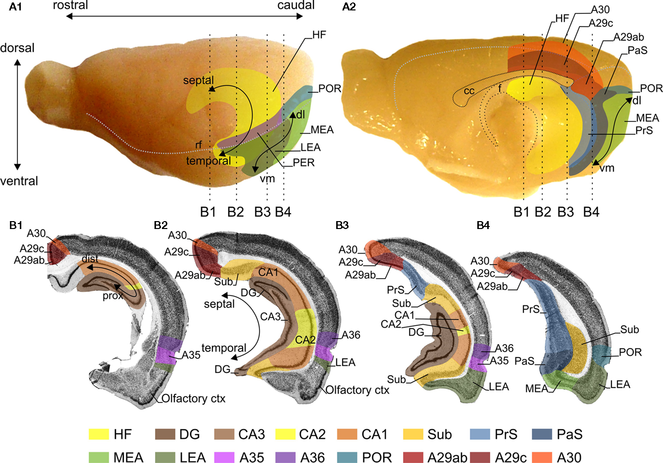
Figure 1. Representations of the retrosplenial cortex (RSC), hippocampal formation (HF) and the parahippocampal region (PHR) in the rat brain. Lateral (A1) and midsagittal (A2) views of the rat brain. The RSC is subdivided into A29ab, A29c, and A30. For orientation a rostrocaudal and dorsoventral axis is indicated (A1). The HF consists of the dentate gyrus (DG), CA3, CA2, CA1, and the subiculum (Sub). The PHR is subdivided into the presubiculum (PrS), parasubiculum (PaS), the entorhinal cortex, which has a lateral (LEA) and a medial (MEA) subdivision, the perirhinal cortex (PER; consisting of Brodmann areas (A)35 and A36) and the postrhinal cortex (POR). For orientation in HF the long or septotemporal axis is used [also referred to as the dorsoventral axis; (A1,B2)]. Another commonly used axis is referred to as the proximodistal axis which indicates a position closer to DG or closer to PHR, respectively (B1). The main axis applied in case of PrS and PaS is also the septotemporal axis, in PER and POR a rostrocaudal axis and in the entorhinal cortex is a dorsolateral-to-ventromedial axis [dl and vm; (A1,A2)]. The dashed vertical lines in panels (A1,A2) indicate the levels of four coronal sections (B1–B4), which are shown in (B). The gray stippled line in (A1) represents the position of the rhinal fissure (rf) and in (A2) they represent the global delineation from the dorsal surface of the brain with the midsagittal and occipital surfaces. (B) Four coronal sections of the rat brain; the levels of these sections are indicated in (A). The subfields of the HF, PHR and RSC are color-coded, see color panel below (B).

TABLE 1

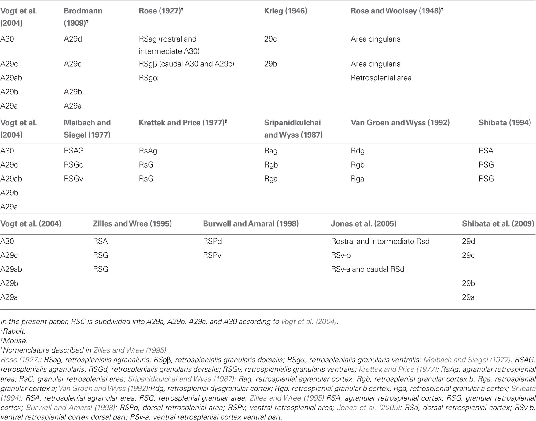
Table 1. Comparison of nomenclatures of the retrosplenial cortex (RSC).

Delineation of RSC

The RSC is a neocortical structure situated in the midline of the cerebrum. It arches around the dorsocaudal half of the corpus callosum in the rat, where it is bordered rostrally by the anterior cingulate cortex, caudoventrally by the PHR and laterally by the parietal and visual cortices. The coordinate system that defines position within the RSC is explained in Figure 1. The delineation of the subareas of RSC is based on cytoarchitectonic features (Figure 2). A29a is the most ventral subdivision and it differs from the dorsally adjacent A29b since it lacks a fully differentiated layered structure. Cytoarchitectonically, A29a has a homogenous layer II/III, while in A29b this layer is divided into a thin superficial densely packed zone and a less dense deeper zone (Vogt and Peters, 1981). A29a and A29b are distinguished from A29c most strikingly in layer III, which in A29ab has cells arranged in bands parallel to the pial surface, while in A29c layer III is thinner and the pyramidal cell bodies are randomly spaced (Van Groen and Wyss, 1990b). An additional way to compare sub-regions is by looking at chemoarchitectonic features. A29ab shows parvalbumin stained cells in layers II, V, and VI, which are not as apparent in A29c (Jones et al., 2005). In AChE stained sections A29c layer IV shows a widening and increased strength of AChE staining compared to layer IV of A29b (Vogt and Peters, 1981; Sripanidkulchai and Wyss, 1987; Van Groen and Wyss, 1990b; Jones et al., 2005). Cytoarchitectonically, A30 shows an abrupt widening and a less dense packing of layer II/III compared to A29b and A29c (Vogt and Peters, 1981; Sripanidkulchai and Wyss, 1987; Van Groen and Wyss, 1992; Jones et al., 2005). Also, A30 layer IV is wider than in A29b/A29c and A30 layer V neuronal cell bodies tend to be larger (Krieg, 1946; Van Groen and Wyss, 1992). In AChE stained sections, layer I–IV of A30 are evenly and darkly stained (Van Groen and Wyss, 1992), whereas in A29c superficial and deep parts of layer I and layer IV are most densely stained (Sripanidkulchai and Wyss, 1987).

FIGURE 2

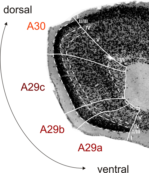
Figure 2. Cytoarchitecture of rat retrosplenial cortex (RSC). Photomicrograph of a coronal section stained for NeuN (high power image taken from the section shown in Figure 1B2), illustrating the cytoarchitectonic characteristics of A29a, A29b, A29c, and A30. A29a has a homogenous layer II/III and lacks fully differentiated deep layers. In A29b layer II/III is divided into a thin superficial densely packed zone and a less dense deeper zone. A29c has a more differentiated layer V and a more equally dense layer II/III compared to A29b and a thinner layer IV compared to A30. A30 shows a widening and a less dense packing of layer II/III and layer V neuronal cell bodies tend to be larger. Layer VI is mostly developed in A30 and A29c and almost absent in A29a and b (for more details see Vogt et al., 2004; Jones et al., 2005).

Nomenclature of HF and PHR

The HF is a C-shaped structure situated bilaterally in the caudal part of the brain. It is subdivided into the dentate gyrus (DG), the Cornu Ammonis (subdivided into CA3, CA2, and CA1), and the subiculum (Sub). The HF consists of three layers, a deep polymorph layer, a more superficial cell layer and on the outside a molecular layer that is almost devoid of neurons. The deep layer is called hilus in the DG and stratum oriens in CA and is not really differentiated in Sub. In DG the cell layer consists of granule cell bodies. In CA and Sub, the cell layer contains pyramidal cells. The superficially positioned molecular layer in DG and Sub is not further subdivided, whereas in CA3, it is divided into three sub-layers: stratum lucidum, stratum radiatum, and stratum lacunosum-moleculare. The lamination of CA2 and CA1 is the same, with the exception that the stratum lucidum is missing.

The PHR borders HF caudally and medially. It is subdivided into the presubiculum (PrS), the parasubiculum (PaS), the entorhinal cortex (EC), further subdivided into the medial and lateral entorhinal area (MEA and LEA respectively), the perirhinal cortex (PER; divided into Brodmann’s areas 35 and 36) and the postrhinal cortex (POR). The PHR is generally described as having six layers. The delineation and the HF–PHR connections are extensively described in earlier publications (Witter and Amaral, 2004; Van Strien et al., 2009). The coordinate system that defines position within the HF and the PHR is explained in Figure 1.

Data Collection and Visualization

A search was performed on publications reporting tract-tracing studies on intrinsic RSC and RSC – HF–PHR connections in PubMed¹ and Embase² (see www.temporal-lobe.com for queries). The following inclusion criteria were used: (1) tract-tracing studies or studies which report intracellular filling of single cells; (2) studies which used healthy, genetically un-altered, untreated adult rats were included; (3) publications written or translated into English or in a language using roman print. The database queries retrieved 816 papers of which 46 contained relevant information. The connectional information was retrieved from these papers, including information from tables and figures, using the following criteria: (1) it was clear where anterogradely filled terminals or retrogradely labeled cell bodies were located; (2) the location of the injection site was clearly described; (3) injection sites did not include multiple brain areas or fiber bundles; (4) lesion studies were discarded; (5) explicitly reported non-excitatory projections were excluded; (6) contralateral projections were excluded. The information about these connections was stored in a custom-made relational database (Microsoft Access; Microsoft Corporation, WA, USA). Before data was entered into this database, the accuracy was verified by at least two of the authors.

Next, results from independent retrograde and anterograde experiments were combined, such that both the layers of origin and termination could be determined. The connections were added to the existing HF–PHR connectome (Van Strien et al., 2009) which was drawn in Visio (Microsoft Corporation, WA, USA) and exported to PDF (Adobe Acrobat Pro; Adobe Systems Inc., CA, USA), see Figure 3 for an overview of the connectome. In total, the database now includes 223 references in 710 records, describing approximately 2600 connections. Compared to the initial interactive connectome, the usability of the current version is improved by adding a search dialog, help section and a tutorial, developed using AcroDialogs and AcroButtons (Windjack Solutions, Inc., OR, USA). Updated and extended support information (e.g., manual, references, and RSC nomenclature) is available on http://www.temporal-lobe.com.

FIGURE 3

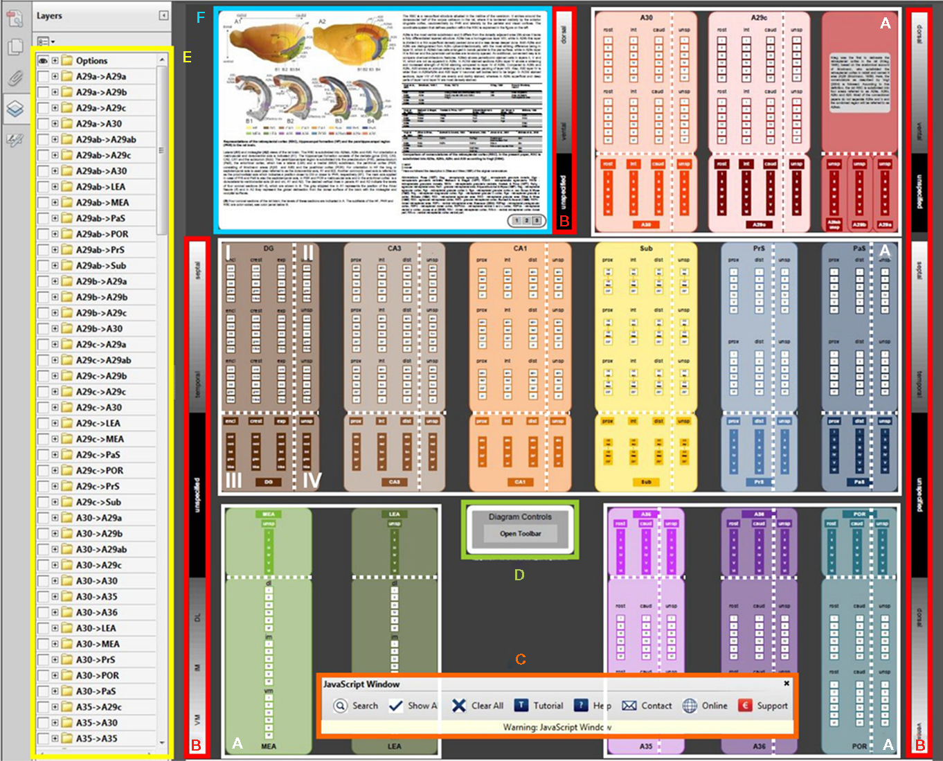
Figure 3. Retrosplenial and hippocampal–parahippocampal connectome. The connectome (see ratbrain_connectome.pdf in Supplementary Material) consists of 14 large, color-coded boxes, which represent the sub-regions of the hippocampal formation, parahippocampal region, and retrosplenial cortex. In this figure, the user interface elements of the connectome are indicated with color-coded outlines and their meaning/purpose is explained. (A) In the white outlines, the 14 anatomical sub-regions are displayed. (B) The 14 anatomical sub-regions are three-dimensionally organized. However, the origin and termination of connections are not always described in full detail in the literature. Therefore, area boxes are divided into four quadrants. Quadrant I has full topological information, whereas the other quadrants have less topological detail. In quadrant I, the vertical axis in the connectome represents the septotemporal axis of dentate gyrus (DG), Cornu Ammonis (CA3 and CA1), subiculum (Sub), presubiculum (PrS) and parasubiculum (PaS), and the dorsoventral axis of medial and lateral entorhinal area (MEA and LEA), retrosplenial cortex (A29 and A30), perirhinal cortex (A35 and A36) and postrhinal cortex (POR). The sidebars (B) display the dorsoventral and septotemporal axes of the anatomical sub-regions. The horizontal axis within quadrant I and III represents the proximodistal axis in CA3, CA1, Sub, PrS, and PaS; the rostrocaudal axis in A29c, A30, A35, A36, and POR and the DG is subdivided into the inner/outer blades and crest region. Within the area boxes, the layers for each specific subarea are outlined. In quadrant II, the information of the vertical axis and the layers are specified, but no details of the horizontal axis are presented. In quadrant III the horizontal axis and the layers are represented, while in quadrant IV, only layer information is present. (C) The interactive connectome allows visualization of detailed connectivity patterns within and between sub-regions. To search for connections, use the search button on the toolbar (C). The toolbar has eight buttons (from left to right): Search for connections, show all connections, clear all connections, a short tutorial on how to search for connections, a help section, contact information, a link to the project website www.temporal-lobe.com and information about how to support this project. (D) If the toolbar is closed, clicking the “open toolbar” button will restore it. (E) After a search is carried out, the retrieved connections will be drawn in the diagram between the appropriate areas and quadrants. Additionally, an eye-icon will appear in the layers panel on the left (E). This is an alphabetically sorted list of “from → to” connection groups that can also be switched on or off manually. In front of each group is a “+” icon. Clicking this icon expands the list of individual connections that make up the group, allowing one to select connections originating from a specific cortical layer or according to a specific three-dimensional projection pattern. (F) The figure panel provides a detailed anatomical description of the retrosplenial cortex, the hippocampal formation and the parahipppcampal region, together with translation tables for nomenclature. Use the buttons in this panel to switch between the figures.

Results

In the following section, the intrinsic connections between RSC subdivisions and connections between RSC subdivisions and the HF and PHR are summarized in a condensed written form (for a condensed overview see Table 2). These connections are also visually presented in the interactive connectome (Supplementary Material).

TABLE 2

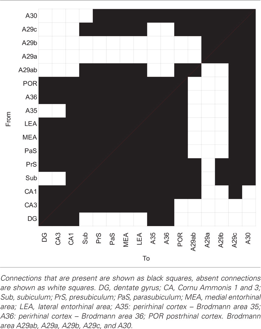
Table 2. Anatomical connections between subareas of the hippocampal formation, the parahippocampal region and the retrosplenial cortex.

Connections within RSC

A29a and A29b

Intrinsic projections are those confined to a defined cytoarchitectonic subarea. In case of A29a and A29b, reports either describe those separately or the two areas have been combined into one A29ab. We therefore deal with the two areas in this section together. The intrinsic projections of A29a originate in layer III–VI and terminate in layers I, II, III, and V. Those of A29b follow a rostral-to-rostral and a caudal-to-caudal pattern. Rostral projections originate in layers II, III, V, and VI and terminate rostrally in all layers. Caudal projections terminate caudally in layers I, II, III, and V (Shibata et al., 2009). The A29a projection to rostral and caudal A29b originates in all cell layers and terminates in layers I, II, III, and V (Shibata et al., 2009). Caudal A29b projects to caudal A29a and rostral A29b projects to rostral A29a and the projections originate in all cell layers and terminate in layers I, II, III, and V (Shibata et al., 2009). The terminal patterns, when combined, are essentially in line with the reported terminal distribution in layers I, III, V, and VI for the combined area A29ab (Van Groen and Wyss, 1990b; Jones et al., 2005; Miyashita and Rockland, 2007).

Both A29a and A29b project to the entire rostrocaudal extent of A29c (Vogt and Miller, 1983; Shibata et al., 2009). Projections that arise from layer V of caudal A29a terminate in layers I, II, III, and VI of the intermediate rostrocaudal and caudal parts of A29c. Rostral A29b projects to rostral and intermediate rostrocaudal A29c, and caudal A29b projects to caudal A29c. Projections originate in layers II, III, V, and VI and terminate in all layers of A29c. When described together (Van Groen and Wyss, 1990b, 2003; Jones et al., 2005; Miyashita and Rockland, 2007), the only striking deviation from the combined separate patterns is that the terminal distribution of the projection from A29ab to rostral A29c is restricted to layers II and III (Van Groen and Wyss, 1990b).

Neurons in layers V and VI of the caudal part of A29a project to caudal levels of A30, terminating in layers I, II, III, and V (Shibata et al., 2009). In case of A29b these projections arise from the entire rostrocaudal extent, but also target caudal portions of A30, showing the same laminar distribution as those of A29a (Vogt and Miller, 1983; Shibata et al., 2009). In line with these observations, the projections from A29ab originate caudally in layer VI and more rostrally in layers III–V projecting to the midrostrocaudal portion of A30 (Van Groen and Wyss, 1990b, 1992; Jones et al., 2005).

A29c

The intrinsic connections of A29c arise from the entire rostrocaudal extent and project to the entire rostrocaudal extent (Vogt and Miller, 1983; Van Groen and Wyss, 2003; Jones et al., 2005; Miyashita and Rockland, 2007; Shibata et al., 2009). These projections originate in layers II, III, V, and VI and terminate in layers I–V. Projections from A29c to caudal A29a exist (Shibata et al., 2009) and the caudal and midrostrocaudal origin is in layer V and that of the rostrally originating projections in layers V and VI. The projections from A29c to A29ab or A29b arise from the entire rostrocaudal extent and project to the entire rostrocaudal extent (Van Groen and Wyss, 1990b, 2003; Jones et al., 2005; Miyashita and Rockland, 2007; Shibata et al., 2009). Rostrally, projections arise from layers V and VI, whereas in caudal A29c projections arise from layers II, III, V, and VI. Termination of these projections in A29b occurs in layers I, II, III, and V. The projection from A29c to A30 originates and terminates in all layers (Vogt and Miller, 1983; Sripanidkulchai and Wyss, 1987; Audinat et al., 1988; Van Groen and Wyss, 1992, 2003; Jones et al., 2005; Shibata et al., 2009). A topographical organization is present, such that rostral A29c projects to rostral and mid-rostrocaudal A30 and caudal A29c projects to the entire rostrocaudal extent of A30.

A30

The intrinsic connections of A30 arise from the entire rostrocaudal extent and project to the entire rostrocaudal extent, whereby layers II–VI project to all layers (Vogt and Miller, 1983; Audinat et al., 1988; Van Groen and Wyss, 1992; Jones et al., 2005; Shibata et al., 2009). Projections to A29a arise from the entire rostrocaudal extent of A30 and terminate caudally (Vogt and Miller, 1983; Shibata et al., 2009). At rostral and intermediate rostrocaudal levels, the projections originate in layer V, whereas caudally the projections arise from layer II–VI. A30 also projects to A29b (Vogt and Miller, 1983; Shibata et al., 2009). This projection arises rostrally from layers V and VI and caudally from layers II–VI. Termination in A29b occurs in layers I, II, III, and V. The caudal and midrostrocaudal projections of A30 to A29ab terminate in all layers (Van Groen and Wyss, 1992; Jones et al., 2005). A30 projects to A29c and the projection does not show a topographical rostrocaudal organization. Projections arise from layers II, III, V, and VI and terminate in all layers of A29c (Vogt and Miller, 1983; Van Groen and Wyss, 1992, 2003; Jones et al., 2005; Shibata et al., 2009).

RSC Projections to the PHR

A29a and A29b

A29ab projects to all subdivisions of PHR. Dense projections exist from A29ab to PrS (Van Groen and Wyss, 1990a,b,d; Shibata, 1994; Jones and Witter, 2007). More specifically, layers II and V of A29ab target PrS layers I, III, V, and VI. The A29ab projection to PrS is topographically organized, such that caudal A29ab targets the entire septotemporal extent of PrS, whereas rostral A29ab targets septal PrS only. The projection to PaS originates in layers II, III, and V and the caudal A29ab projects to the whole septotemporal axis of the PaS (Van Groen and Wyss, 1990a,b; Shibata, 1994; Jones and Witter, 2007). The projections to PER originate in caudal and intermediate rostrocaudal A29ab and terminate in layers V and VI (Shibata, 1994; Jones and Witter, 2007). The POR projection originates in layer II and V and terminates in all layers (Jones and Witter, 2007). The projection to LEA layers I, II, III, V, and VI and MEA layers I, V, and VI originates in caudal A29ab (Jones and Witter, 2007).

A29c

A29c also projects to all subdivisions of PHR. The projection to PrS is topographically organized along the rostrocaudal axis, such that caudal A29c projects to the entire septotemporal extent of PrS, intermediate A29c projects to intermediate and septal PrS, whereas rostral A29c only projects to septal PrS (Meibach and Siegel, 1977; Vogt and Miller, 1983; Van Groen and Wyss, 1990a,d, 2003; Shibata, 1994; Gonzalo-Ruiz and Bayona, 2001; Jones and Witter, 2007). Projections to temporal PrS originate in layers II and V, whereas projections that terminate in septal PrS are reported to originate only in layer V. Termination has been reported in all layers of PrS. The projection to PaS originates in layer V and terminates in all layers (Vogt and Miller, 1983; Finch et al., 1984; Van Groen and Wyss, 1990a; Shibata, 1994; Jones and Witter, 2007). Whether or not this projection shows a topographical organization is unclear. The projection to PER that arises from midrostrocaudal A29c terminates in layer V and VI of PER, whereas the caudal A29c projection terminates in all layers of PER (Guldin and Markowitsch, 1983; Shibata, 1994; Jones and Witter, 2007). The projection to POR originates in layers II and V of A29c and terminates in all layers (Burwell and Amaral, 1998; Jones and Witter, 2007). Both MEA and LEA are targeted by projections that originate in caudal A29c. Termination in EC has been reported to include both superficial layers and deep layers (Shibata, 1994; Jones and Witter, 2007).

A30

Similar to A29ab and A29c, A30 also projects to all subdivisions of the PHR. The projections to PrS originate in layers II and V and terminate in layers I, II, III, V, and VI (Vogt and Miller, 1983; Van Groen and Wyss, 1990a, 1992; Shibata, 1994; Jones and Witter, 2007). The topographical organization of this projection is such that rostral A30 projects to septal PrS, whereas caudal and midrostrocaudal A30 project to the entire septotemporal extent of PrS. The projection to PaS originates along the entire rostrocaudal extent of A30 (Vogt and Miller, 1983; Van Groen and Wyss, 1992; Shibata, 1994; Jones and Witter, 2007). The layers from which these projections originate have not been determined, and the projections terminate in all layers of PaS. The projections to PER originate from the rostrocaudal extent of A30. Rostral A30 projections to PER show terminal labeling in layers V and VI. Caudal projections originate in layers II, III, and V and terminate in all layers of PER (Deacon et al., 1983; Shibata, 1994; Burwell and Amaral, 1998; Jones and Witter, 2007). A30 projections to POR originate in layers II and V and terminate in all layers of POR. No topographical organization has been reported (Burwell and Amaral, 1998; Jones and Witter, 2007). A30 to EC projections show the following pattern: Layer V of A30 projects to all layers of MEA. However, caudal A30 was shown to project to LEA and MEA layers V and VI, whereas intermediate rostrocaudal A30 was shown to project to MEA layers I, II, and III (Van Groen and Wyss, 1992; Shibata, 1994; Burwell and Amaral, 1998; Jones and Witter, 2007).

PHR Projections to the RSC

A29a and A29b

Some PHR sub-regions send return projections to A29ab. Septal and temporal PrS layer V neurons project to A29ab layers I–V (Finch et al., 1984; Van Groen and Wyss, 1990a,b,d). A projection from EC to A29ab has been reported, but topographical information for this projection is absent (Miyashita and Rockland, 2007). Although PaS, PER, and POR receive connections from A29ab, return projections have not been described.

A29c

Neurons in PrS layer V project to layers I and III of A29c. Septal PrS projections terminate in the whole rostrocaudal extent of A29c (Vogt and Miller, 1983; Finch et al., 1984; Van Groen and Wyss, 1990a,d, 2003). Neurons in PaS layer V project to layer II and III of A29c (Vogt and Miller, 1983; Finch et al., 1984). Similarly, projections from PER (A35, A36) and POR to A29c have been reported, but no additional information about these projections is available (Agster and Burwell, 2009). Finally, layer V of both LEA (Agster and Burwell, 2009) and MEA (Frohlich and Ott, 1980; Insausti et al., 1997; Agster and Burwell, 2009) project to A29c. MEA is known to project to layers I, II, and IV of A29c (Frohlich and Ott, 1980; Insausti et al., 1997).

A30

Neurons in layers V and VI of septal PrS project to layers I, III, IV, and V of A30 (Vogt and Miller, 1983; Finch et al., 1984; Witter et al., 1990; Van Groen and Wyss, 1992). PaS layer V projects to A30, but the layers of termination are unknown (Vogt and Miller, 1983). A35 and A36 also project to A30 (Agster and Burwell, 2009), where caudal A36 projects to caudal A30. POR projects to A30, but layer specific information is absent (Agster and Burwell, 2009). Finally, both LEA (Agster and Burwell, 2009) and MEA (Insausti et al., 1997; Agster and Burwell, 2009) have been reported to project to A30, but only for MEA a termination in layers I and II of A30 has been described (Insausti et al., 1997).

RSC Projection to the HF

A29a and A29b

Neurons in layer V of A29ab project to Sub in the HF (Van Groen and Wyss, 1990b; Shibata, 1994). This projection is topographically organized such that caudal A29ab projects to temporal Sub, where termination occurs in the stratum moleculare and stratum pyramidale, whereas rostral and intermediate A29ab projects to intermediate septotemporal levels of Sub, where termination occurs in the stratum pyramidale.

A29c

Also for A29c, Sub is the only HF target (Meibach and Siegel, 1977; Shibata, 1994; Gonzalo-Ruiz and Bayona, 2001; Van Groen and Wyss, 2003). This projection is topographically organized along the rostrocaudal axis, such that rostral A29c projects to septal and intermediate septotemporal levels of Sub, intermediate A29c projects to intermediate septotemporal levels and caudal A29c projects to temporal and intermediate septotemporal levels of Sub. Caudal projections to temporal Sub have been described to terminate in stratum moleculare and stratum pyramidale, whereas projections from rostral A29c to intermediate septotemporal Sub terminate in stratum pyramidale.

HF Projections to the RSC

A29a and A29b

The HF projections to A29ab originate in Sub and CA1. Sub projections to A29ab terminate in layers I, II, and III and mimic the topographical organization of the retrosplenial projections to Sub. The projection from CA1 to A29ab originates from the septal portion (Van Groen and Wyss, 1990b; Naber and Witter, 1998; Miyashita and Rockland, 2007).

A29c

The HF projections to A29c also originate in Sub and CA1. The proximal part of the septal Sub projects to rostral A29c. Intermediate septotemporal and distal Sub project to caudal A29c (Vogt and Miller, 1983; Finch et al., 1984; Naber and Witter, 1998; Van Groen and Wyss, 2003; Miyashita and Rockland, 2007). These projections typically terminate in layers II and III. No information about temporal Sub to A29c projections has been published. The distal portion of septal CA1 also projects to A29c. The projection originates in neurons in stratum pyramidale and at the border between stratum moleculare and stratum radiatum and terminates in layers II, III, and IV (Meibach and Siegel, 1977; Van Groen and Wyss, 1990c, 2003; Naber and Witter, 1998; Miyashita and Rockland, 2007).

A30

The HF projections to A30 only originate in Sub. The distal portion of the septal Sub, as well as the intermediate proximodistal portion of intermediate septotemporal Sub project to layers I and II of A30 (Vogt and Miller, 1983; Finch et al., 1984; Kohler, 1985; Witter et al., 1990).

Summary of Intrinsic RSC Connections

There are strong intrinsic connections within the RSC subdivisions. All rostrocaudal levels within both A29c and A30 issue projections to their respective rostrocaudal extents. A29b projections have a strict topography from rostral-to-rostral and from caudal-to-caudal; A29a only has a caudal-to-caudal projection. There are also strong reciprocal connections between the RSC subdivisions. All rostrocaudal levels of one subdivision project to all rostrocaudal levels of all other subdivisions, but there are some exceptions: (1) caudal A29a projects only to caudal A29b, A29c, and A30; (2) caudal A29b does not project to rostral A29c; (3) rostral A29c does not project to caudal A30; (4) rostral and midrostrocaudal A30 only projects to caudal A29b and the return projection from A29b only terminates in caudal A30.

Summary of RSC – HF/PHR Connections

The RSC projects to all PHR subdivisions and Sub. Only the projections of RSC to PrS and Sub show a topographical organization such that the rostrocaudal axis of origin in RSC correlates to a septotemporal terminal distribution in PrS and Sub. The projections to PrS are among the densest of RSC–PHR connections (Jones and Witter, 2007) and this is particularly true for projections from caudal RSC (Shibata, 1994). A topographical pattern for reciprocal connections has not been identified. Areas 30 and 29c receive input from the whole PHR and Sub, while PrS and Sub are the only areas which project to A29b and A29ab. Dorsal CA1 projects only to A29ab and A29c.

Discussion

The connectome of the rat brain should describe all network elements and connections in a clear and comprehensible way. Compared to the comprehensiveness that a connectome implies, current knowledge is in its infancy. When considering the vast number of neurons in the rat nervous system and their connections, together with the currently available technologies to collect and handle information about them, creating a connectome is an expensive, time consuming, and complicated task. Scientists will eventually have a comprehensive map of the rat brain available, and just like the usefulness of an easily accessible map of all the roads in the world, such a connectome will be an indispensible foundation for basic and applied neurobiological research (Sporns et al., 2005). Therefore, regardless of the complexity and duration of the undertaking to create a connectome, the challenge to create a connectome of the mouse, rat, monkey, and human brain has been readily accepted by scientists [e.g., Brain Architecture Management System (BAMS), CoCoMac, The Rodent Brain Workbench, BrainNavigator, Blue Brain Project, The Allen brain atlas, Neuroscience Information Network (NIF). For a complete overview of projects see the International Coordinating Facility (INCF)].

With this publication, we present the current version of our partial rat brain connectome, which to the best of our knowledge represents all current information on the ipsilateral pathways within and between the HF, PHR, and RSC. A different approach from that of a traditional meta-analysis was taken, to create this connectome. In a traditional meta-analysis, typically only a subset of data is selected, summarized, and organized according to the author’s views. The resulting reduction in detail of anatomical networks is useful for creating scientific hypotheses, but contradicts with a fundamental characteristic of a connectome: to be an exhaustive knowledge resource. Therefore, we chose the approach to present the anatomical data of the selected regions in the fullest available detail, which allows scientists to prune this information themselves to match their hypotheses, or design competing anatomical hypotheses.

We realize that the current state of knowledge is not exhaustive and hence one could argue that the connectome presented here is not a real connectome. Nevertheless, the connectome presented here provides the best approximation of a full connectome at the current point in time. With future publications we aim to continually update and expand the database. Still, users of connectomes should always keep a perspective on where the current state of knowledge stands compared to having absolute knowledge. For this reason, this discussion will first touch upon some of the challenges of anatomical connectomes that remain to be resolved, after which the potentials of connectomes will be exemplified using the information presented in this review.

Challenge 1: Borders in the Brain

Combining data produced by many researchers, over 100 years, using many different techniques in a great number of tract-tracing experiments, leads to a number of challenges on demarcation of brain areas and designation of names in research reports. Such nomenclature issues exist not only for the RSC, but for almost all brain regions. These issues have arisen because different histological techniques produce different definitions of borders in the brain, or simply because researchers disagree on the demarcation.

Krieg (1946) was the first to delineate the RSC in the rat. Based on the nomenclature of Brodmann (1909) who subdivided the RSC in rabbit and dubbed it A29, Krieg divided it into a ventral subdivision (A29b) and a dorsal subdivision (A29c) in the rat (Table 1). In the 1970s of the last century, Krettek and Price (1977) divided the RSC in a granular and an agranular subdivision, the RsG and the RsAg. The granular part was further differentiated into a dorsal and a ventral part by Meibach and Siegel (1977). Vogt and Peters (1981) divided the granular subdivision into three areas, A29a, b, and c based on termination patterns of callosal fibers. In this century, Jones et al. (2005), Jones and Witter (2007) delineated the RSC borders based on parvalbumin stainings and classified the most caudal part of A29ab with A30 into the dorsal retrosplenial cortex (RSd). Although no standardization of nomenclatures has become apparent, dealing flexibly with the diverse nomenclatures may allow to efficiently generate inspiring insights into the organization of the RSC. Therefore, in the current HF–PHR–RSC connectome, we selected one nomenclature to express ourselves. For RSC we used the nomenclature of Vogt et al. (2004) and for HF–PHR the nomenclature of Witter and Amaral (2004). We provided what we call a “Rosetta table” of nomenclatures. The “Rosetta table” of nomenclatures is a necessary translation tool that lists all available nomenclatures (for a given structure in a given species) and facilitates translating between different nomenclatures. For such translations, different methods have been developed, and we applied careful comparison of all cyto- and chemoarchitectural features described in the original publications (Bota and Swanson, 2010).

Challenge 2: Level of Detail

Aspecific reporting

Even when using technically advanced methods to clarify projection patterns, the usefulness of a scientific report on anatomical connections depends to a great extent on how detailed the authors report their results and the way they present the data in figures to support their observations. When reviewing the projections from RSC to HF and PHR, only in a few studies information was provided on the layers of origin or termination, or specific projection patterns. For example, projections from A29ab, A29c, and A30 to LEA and MEA exist (Van Groen and Wyss, 1992; Burwell and Amaral, 1998; Jones and Witter, 2007) and although LEA and MEA show an overall dorsolateral-to-ventromedial connectional and functional gradient, none of these reports provide comparable termination information. Even less specific accounts inform us that RSC projects to the EC, without indicating if the projections terminated in the lateral or medial subdivision (Audinat et al., 1988; Van Groen and Wyss, 1990b; Shibata, 1994). This is regrettable, since more detailed information about the origin and termination could be related to the function of a connection. It is known that functional differences between the LEA and MEA exist. Neurons in the MEA exhibit spatial selectivity, while LEA cells display only weak spatial modulation (Fyhn et al., 2004; Hargreaves et al., 2005). Since projections from RSC to EC mainly target MEA, it could be hypothesized that this input is relevant to spatial firing properties of MEA neurons. Unfortunately, the current level of detail is such that almost nothing is known about the topography and lamination of the HF and PHR projections to the RSC and vice versa. In our connectome, this information is displayed as connecting areas with an unspecified origin or termination. This lack of detailed information makes it difficult to predict the function of projections or small networks. Fortunately, more advanced methods to explore brain networks are continuously being developed, making it likely that future expansions of the connectome can include for example, information about the nature of postsynaptic targets or the distribution of synapses on the dendritic tree.

Displaying layer specificity

To obtain information about layer specificity of projections, ideally anterograde and retrograde tract-tracing experiments are combined. For example, an anterograde tracer injection is placed in midrostrocaudal A30, thereby discovering regions of termination including layers I, II, III, and V of rostral A29c. This experiment should be completed by placing a retrograde tracer in rostral A29c, to reveal the layers of origin of this projection in midrostrocaudal A30, i.e., layer II, III, V, and VI (Shibata et al., 2009). A strength of our current approach is that a database of connections allows easy combination of anterograde and retrograde experiments, even across publications. But when representing this information in a connectome, should one draw projections from all origin layers to all target layers, or could it be that a more specific pattern exists, e.g., that layer II cells only project to layer V of the target region? Therefore, only when single cells are fully traced (e.g., Honda et al., 2011), one can accurately describe layer specificity of projections.

Displaying projection topographies

Apart from layer specificity, projections may be topographically organized. For example, the rostral RSC projects weaker to EC than caudal RSC. Often, such topographies show a gradient in projection strength, but one cannot rigorously claim that only caudal RSC projects to EC. In the current version of our connectome, such topographies are not visible since no information on relative density is included. We chose this approach, in view of the risk that by emphasizing some brain connections over others, the less emphasized ones may be erased from the scientific working memory. However, users should not forget that brain connections typically have different strengths and may show topographical gradients that are not apparent in the interactive connectome.

Challenge 3: Functional Connectivity

When using our connectome, it is important to keep in mind that two connections symbolized by two similar looking lines may be different from one another for a number of reasons.

Excitatory – inhibitory, modulation

Our connectome is based on tract-tracing data and thus comes with certain limitations related to this technique. One important limitation is that tract-tracing does not reveal if a connection is excitatory or inhibitory, whereas this information is of functional relevance. By combining immunohistochemistry with either confocal or electron microscopy, it can be established if a projection is excitatory or inhibitory (Van Haeften et al., 1997). Alternatively, electrophysiological data can help determine this functional property and such information will eventually be incorporated into the connectome.

In our current connectome, known GABA-ergic connections are not specifically included, although some projections are likely GABA-ergic. There is a dense GABA-ergic projection from CA1 to the RSC, starting from all layers except the stratum lacunose-moleculare (Miyashita and Rockland, 2007). Non-pyramidal cells, which could be GABA-ergic, of the septal Sub are projecting to layer I of the RSC as well (Van Groen and Wyss, 1992, 2003; Miyashita and Rockland, 2007). Hippocampal GABA-ergic neurons also project intra-hippocampally (Jinno, 2009). Inhibitory GABA-ergic projections are involved in regulation of neural oscillations (Somogyi and Klausberger, 2005). Theta oscillations (4–12 Hz) for instance, have been postulated to support memory formation in the HF and the cortex (Klausberger et al., 2003). Theta oscillations have also been recorded in the RSC (Borst et al., 1987; Talk et al., 2004) and are in coherence with oscillations in CA1 (Young and Mcnaughton, 2009). Although this coherence may be a product of volume conduction from the hippocampus, the GABA-ergic projections from CA1 and Sub to RSC could play a role as well.

Weak – strong connections

Most anatomical reports contain subjective descriptions of the strengths of projections. Such subjective reports are impossible to quantify and therefore such information cannot be incorporated in the connectome. Yet, in reality differences in strengths exist. For instance, the projection from A29ab to MEA is reported to terminate in both superficial and deep layers. When assessing this connection in detail, clear differences between superficial and deep layers exist. There is dense terminal labeling in layer V of MEA, whereas terminal labeling in layer III is very light (Jones and Witter, 2007). Therefore, it would be reasonable to suggest that the major effect of A29ab on MEA is mediated through layer V, not through layer III. Moreover a strong projection could arise from a small number of neurons that supply a highly collateralized terminal plexus, but a similarly strong projection may also result from many cells sending less collateralized axons to the target area. This type of information is almost never available in the literature. Yet a connectome ideally would describe this information.

Challenge 4: Not Reported or No Connection?

Another challenge is how to interpret “negative information.” There are two types of negative information: (1) there is data that indicate that a connection between area A and area B is very unlikely, or (2) a connection between area A and area B was not reported, but may exist. For example, the current literature assessment shows that A29c and A29ab both project to Sub, whereas data on a projection from A30 to Sub are lacking. Should one now conclude that a projection from A30 to Sub is not present in the rat brain, or could it be that this projection is present, but perhaps remained undetected or was detected but not reported? This issue has been dealt with in other databases, where connections that are explicitly reported to not exist have been collated (Stephan et al., 2000; Bota and Arbib, 2004). In a future version of our database we plan to implement a similar solution. Currently, some caution is required when drawing conclusions on the basis of the connectome alone.

Challenge 5: Inclusion of Incorrect Data

Although it is assumed that researchers aim to report as accurately as possible the results of their tract-tracing experiments, it does not exclude the possibility that brain connections are reported that do not exist. Tract-tracing techniques were much refined over time, such that injections of modern tracers such as Phaseolus Vulgaris-leucoagglutinin or biotinylated dextran-amine can now be injected region or cell layer selective (Gerfen and Sawchenko, 1984; Wouterlood and Jorritsma-Byham, 1993). Compared to modern tract-tracing studies, many of the old reports are coarse and provide little information for the current connectome. Such reports are only of interest when they seem valid and provide the only available source of knowledge about a particular connection.

A bigger problem occurs when a report provides many connection details, but too little evidence is presented to confirm the claims of authors. In such cases, one can only trust the author’s interpretation of the data, in the absence of proof against it. However, when sufficient proof against the existence of a connection is available, such information is registered in our connection database, but excluded or removed from the connectome. An example of a connection that was reported but is not in the current connectome is based on an injection in A30 and A29c with terminal labeling in Sub, septal PrS and PaS (Vogt and Miller, 1983) or an injection in Sub, PrS, and CA1 (Long et al., 1995). These data were excluded from the connectome because the tracer injections covered more than one defined region or targeted fiber bundles. Another possible confounder occurs if described results do not match those in the referred figures or tables. In such cases they were either corrected to match the figure or table or if that was impossible, they were excluded entirely. Nevertheless, such “false positive” reports are taken up in the reference tables on our website, which displays in which papers connections were reported, such that scientists can evaluate such reports for themselves.

Advantage 1: Education

Apart from scientific value, a connectome is useful as an educational tool to get an overview of an ever increasing amount of literature. Instead of having to search through many papers, basic anatomical facts such as the three dimensional organization of a structure, but also complex issues such as differences in nomenclature and perhaps most complex, the numerous connections between brain regions, are neatly organized, such that users can easily get an exhaustive overview of information at the level of detail that they choose. This is useful for novice researchers who just started to learn about the organization of the brain, as well as researchers who wish to expand their research into new brain regions that are charted in the connectome.

Advantage 2: Scientific Value

There are several scientific uses of connectomes. A connectome can help detect knowledge gaps, it will improve the interpretation of experimental results and may facilitate the design of new experiments. Depending on the level of detail of the available information, the scientific value varies between these uses. If little information is available, a connectome will mainly help detect knowledge gaps. When a reasonable amount of details are known, it will help better understand completed experiments. The true potential of a connectome becomes apparent only when the level of detail of information goes beyond the point where one can easily keep track of all the known facts.

Detection of knowledge gaps

Even though the current connectome may look overwhelming already, a close look immediately points to gaps in our knowledge. For example, there are no experiments evaluating the topographical organization of the connections between A29a or A29b and HF–PHR. Anterograde or retrograde injections in A29a or A29b and the topography of terminating patterns or labeling of neurons in PHR have not yet been described. Similarly, injections in HF–PHR and descriptions of the terminating patterns in A29a or A29b are missing. Another example concerns the topography of the projection from PrS to RSC. It is known that temporal PrS projects specifically to A29ab, whereas septal PrS projects to all RSC subdivisions. It is likely that a more specified topography exists, for example along the rostrocaudal axis of RSC, but such information is presently unknown.

Understanding experiments

Another useful scientific application is the graphical representation of hypotheses. Sometimes it is easier to understand a hypothesis by looking at a graphical representation of the connections. For example, it was hypothesized that information transfer between the RSC and PHR–HF is crucial for adequate navigation and spatial memory. This is supported by the observation that extensive lesions, including A29ab and A29c disrupt spatial memory tasks (Pothuizen et al., 2010). However, it is also likely that different subdivisions of the RSC have different roles in navigation and spatial memory, since lesioning A29c and A30 results in impaired performance on spatial learning tests, whereas selective lesions of A29ab do not interfere with the performance in spatial tasks (Van Groen et al., 2004; Vann and Aggleton, 2005). When looking at the connectome, it can be seen that A29ab receives information from septal and temporal PrS, septal and temporal Sub and septal CA1, whereas A30 and A29c receive inputs from LEA, MEA, A35, A36, POR, PaS, next to input from PrS, Sub, and CA1. These connectional differences may partially explain the lesion data, but likely will also lead to new concepts or new experiments.

Another example of an inferred experiment, based on the connectome follows from the topography observed in the RSC – HF–PHR projections. The traditional emphasis on the topography of RSC – HF–PHR projections relies on the observation that there is a gradient in the RSC to HF–PHR projections, such that rostral RSC (A29c) projects primarily to septal parts of HF–PHR (PrS) and caudal RSC (A29c/A30) projects both to septal and temporal HF–PHR (PrS). Upon close inspection, a more striking topography is apparent in the projections of Sub to A29c. The transverse axis of Sub relates to the rostrocaudal axis in A29c such that proximal Sub projects to the rostral part of A29c and distal Sub projects to the caudal of A29c. This topography could be of functional relevance, since LEA projects to proximal parts of Sub, whereas MEA projects distally (Tamamaki and Nojyo, 1995; Naber et al., 2001; Baks-Te Bulte et al., 2005). This suggests that MEA related input is selectively transferred to caudal portions of A29c and LEA related input to more rostral levels. Since the projections from CA1 to Sub follow a matching proximodistal organization and CA1 also projects to A29c, it would be of interest to know whether the CA1 to A29c projection is in register, such that distal CA1 projects to rostral A29c and proximal CA1 projects to caudal A29c.

The current connectome, as presented here, is far from complete and differences exist in the amount of information that is available about anatomical demarcation and connectivity of different brain areas. The HF connectivity is relatively well covered, followed by the PHR – HF connections and least is known about HF – RSC connectivity. As indicated, the amount of available information is largely decisive for the type of questions a connectome can assist with. We do not see these issues as shortcomings undermining the value of this approach. Connectomes can continuously be updated and extended and therefore will always provide an exhaustive and up to date account of the current knowledge. These two factors precisely define the value of connectomes. Moreover, anatomical connectivity characterizes the brain at an intermediate information level, allowing to easily link this to, e.g., functional properties of individual cells or effective connectivity (Friston, 2011). Such linking is a key prerequisite to fully understand brain function. A connectome therefore does not only describe the architecture of the brain, it also is a key linking system to understand brain function at multiple scales.

Conflict of Interest Statement

The authors declare that the research was conducted in the absence of any commercial or financial relationships that could be construed as a potential conflict of interest.

Acknowledgments

We like to thank Ingrid Riphagen for designing and performing the initial literature searches. Niels M. van Strien was supported by the Norwegian Research Council, Independent projects – Biology and Biomedicine grant number 197245. Menno P. Witter and Jørgen Sugar received support from the Kavli Foundation and the Norwegian Research Council, centre of excellence grant number 145993.

Supplementary Material

The Supplementary Material for this article can be found online at http://www.frontiersin.org/Neuroinformatics/10.3389/fninf.2011.00007/abstract

Footnotes

1. ^www.PubMed.gov
2. ^www.embase.com

References

Agster, K. L., and Burwell, R. D. (2009). Cortical efferents of the perirhinal, postrhinal, and entorhinal cortices of the rat. Hippocampus 19, 1159–1186.

Pubmed Abstract | Pubmed Full Text | CrossRef Full Text

Audinat, E., Conde, F., and Crepel, F. (1988). Cortico-cortical connections of the limbic cortex of the rat. Exp. Brain Res. 69, 439–443.

Pubmed Abstract | Pubmed Full Text | CrossRef Full Text

Baks-Te Bulte, L., Wouterlood, F. G., Vinkenoog, M., and Witter, M. P. (2005). Entorhinal projections terminate onto principal neurons and interneurons in the subiculum: a quantitative electron microscopical analysis in the rat. Neuroscience 136, 729–739.

Pubmed Abstract | Pubmed Full Text | CrossRef Full Text

Boccara, C. N., Sargolini, F., Thoresen, V. H., Solstad, T., Witter, M. P., Moser, E. I., and Moser, M. B. (2010). Grid cells in pre- and parasubiculum. Nat. Neurosci. 13, 987–994.

Pubmed Abstract | Pubmed Full Text | CrossRef Full Text

Borst, J. G., Leung, L. W., and Macfabe, D. F. (1987). Electrical activity of the cingulate cortex. II. Cholinergic modulation. Brain Res. 407, 81–93.

Pubmed Abstract | Pubmed Full Text | CrossRef Full Text

Bota, M., and Arbib, M. A. (2004). Integrating databases and expert systems for the analysis of brain structures: connections, similarities, and homologies. Neuroinformatics 2, 19–58.

Pubmed Abstract | Pubmed Full Text | CrossRef Full Text

Bota, M., and Swanson, L. W. (2010). Collating and curating neuroanatomical nomenclatures: principles and use of the brain architecture knowledge management system (BAMS). Front. Neuroinform. 4:3. doi: 10.3389/fninf.2010.00003.

Pubmed Abstract | Pubmed Full Text | CrossRef Full Text

Brodmann, K. (1909). Vergleichende Lokalisationslehre der Grosshirnrinde in ihren Prinzipien dargestellt auf Grund des Zellenbauers. Leipzig: Verlag von Johann Ambrosius Barth.

Buckner, R. L., Andrews-Hanna, J. R., and Schacter, D. L. (2008). The brain’s default network: anatomy, function, and relevance to disease. Ann. N. Y. Acad. Sci. 1124, 1–38.

Pubmed Abstract | Pubmed Full Text | CrossRef Full Text

Burwell, R. D., and Amaral, D. G. (1998). Cortical afferents of the perirhinal, postrhinal, and entorhinal cortices of the rat. J. Comp. Neurol. 398, 179–205.

Pubmed Abstract | Pubmed Full Text | CrossRef Full Text

Chen, L. L., Lin, L. H., Green, E. J., Barnes, C. A., and Mcnaughton, B. L. (1994). Head-direction cells in the rat posterior cortex. I. Anatomical distribution and behavioral modulation. Exp. Brain Res. 101, 8–23.

Pubmed Abstract | Pubmed Full Text | CrossRef Full Text

Cho, J., and Sharp, P. E. (2001). Head direction, place, and movement correlates for cells in the rat retrosplenial cortex. Behav. Neurosci. 115, 3–25.

Pubmed Abstract | Pubmed Full Text | CrossRef Full Text

Cooper, B. G., and Mizumori, S. J. (1999). Retrosplenial cortex inactivation selectively impairs navigation in darkness. Neuroreport 10, 625–630.

Pubmed Abstract | Pubmed Full Text | CrossRef Full Text

Crick, F., and Koch, C. (2003). A framework for consciousness. Nat. Neurosci. 6, 119–126.

Pubmed Abstract | Pubmed Full Text | CrossRef Full Text

Deacon, T. W., Eichenbaum, H., Rosenberg, P., and Eckmann, K. W. (1983). Afferent connections of the perirhinal cortex in the rat. J. Comp. Neurol. 220, 168–190.

Pubmed Abstract | Pubmed Full Text | CrossRef Full Text

Finch, D. M., Derian, E. L., and Babb, T. L. (1984). Afferent fibers to rat cingulate cortex. Exp. Neurol. 83, 468–485.

Pubmed Abstract | Pubmed Full Text | CrossRef Full Text

Friston, K. J. (2011). Functional and effective connectivity: a review. Brain Connect. 1, 13–36.

Frohlich, J., and Ott, T. (1980). Autoradiographic analysis of projections from the medial entorhinal cortex to limbic areas. Folia Morphol. (Praha) 28, 240–245.

Pubmed Abstract | Pubmed Full Text

Fyhn, M., Molden, S., Witter, M. P., Moser, E. I., and Moser, M. B. (2004). Spatial representation in the entorhinal cortex. Science 305, 1258–1264.

Pubmed Abstract | Pubmed Full Text | CrossRef Full Text

Gerfen, C. R., and Sawchenko, P. E. (1984). An anterograde neuroanatomical tracing method that shows the detailed morphology of neurons, their axons and terminals: immunohistochemical localization of an axonally transported plant lectin, Phaseolus vulgaris leucoagglutinin (PHA-L). Brain Res. 290, 219–238.

Pubmed Abstract | Pubmed Full Text | CrossRef Full Text

Gonzalo-Ruiz, A., and Bayona, I. (2001). Localization of excitatory amino acid and neuropeptide markers in neurons of the subicular complex projecting to the retrosplenial granular cortex of the rat. Eur. J. Anat. 5, 119–132.

Greicius, M. D., Supekar, K., Menon, V., and Dougherty, R. F. (2009). Resting-state functional connectivity reflects structural connectivity in the default mode network. Cereb. Cortex 19, 72–78.

Pubmed Abstract | Pubmed Full Text | CrossRef Full Text

Guldin, W. O., and Markowitsch, H. J. (1983). Cortical and thalamic afferent connections of the insular and adjacent cortex of the rat. J. Comp. Neurol. 215, 135–153.

Pubmed Abstract | Pubmed Full Text | CrossRef Full Text

Hargreaves, E. L., Rao, G., Lee, I., and Knierim, J. J. (2005). Major dissociation between medial and lateral entorhinal input to dorsal hippocampus. Science 308, 1792–1794.

Pubmed Abstract | Pubmed Full Text | CrossRef Full Text

Henderson, V. W., Mack, W., and Williams, B. W. (1989). Spatial disorientation in Alzheimer’s disease. Arch. Neurol. 46, 391–394.

Pubmed Abstract | Pubmed Full Text

Honda, Y., Furuta, T., Kaneko, T., Shibata, H., and Sasaki, H. (2011). Patterns of axonal collateralization of single layer V cortical projection neurons in the rat presubiculum. J. Comp. Neurol. 519, 1395–1412.

Pubmed Abstract | Pubmed Full Text | CrossRef Full Text

Insausti, R., Herrero, M. T., and Witter, M. P. (1997). Entorhinal cortex of the rat: cytoarchitectonic subdivisions and the origin and distribution of cortical efferents. Hippocampus 7, 146–183.

Pubmed Abstract | Pubmed Full Text | CrossRef Full Text

Jinno, S. (2009). Structural organization of long-range GABAergic projection system of the hippocampus. Front. Neuroanat. 3:13. doi: 10.3389/neuro.05.013.2009

Pubmed Abstract | Pubmed Full Text | CrossRef Full Text

Jones, B. F., Groenewegen, H. J., and Witter, M. P. (2005). Intrinsic connections of the cingulate cortex in the rat suggest the existence of multiple functionally segregated networks. Neuroscience 133, 193–207.

Pubmed Abstract | Pubmed Full Text | CrossRef Full Text

Jones, B. F., and Witter, M. P. (2007). Cingulate cortex projections to the parahippocampal region and hippocampal formation in the rat. Hippocampus 17, 957–976.

Pubmed Abstract | Pubmed Full Text | CrossRef Full Text

Klausberger, T., Magill, P. J., Marton, L. F., Roberts, J. D., Cobden, P. M., Buzsaki, G., and Somogyi, P. (2003). Brain-state- and cell-type-specific firing of hippocampal interneurons in vivo. Nature 421, 844–848.

Pubmed Abstract | Pubmed Full Text | CrossRef Full Text

Kohler, C. (1985). Intrinsic projections of the retrohippocampal region in the rat brain. I. The subicular complex. J. Comp. Neurol. 236, 504–522.

Pubmed Abstract | Pubmed Full Text | CrossRef Full Text

Krettek, J. E., and Price, J. L. (1977). The cortical projections of the mediodorsal nucleus and adjacent thalamic nuclei in the rat. J. Comp. Neurol. 171, 157–191.

Pubmed Abstract | Pubmed Full Text | CrossRef Full Text

Krieg, W. J. (1946). Connections of the cerebral cortex; the albino rat; structure of the cortical areas. J. Comp. Neurol. 84, 277–323.

Pubmed Abstract | Pubmed Full Text | CrossRef Full Text

Long, Y., Hardwick, A. L., and Frederickson, C. J. (1995). Zinc-containing innervation of the subicular region in the rat. Neurochem. Int. 27, 95–103.

Pubmed Abstract | Pubmed Full Text | CrossRef Full Text

Maguire, E. A. (2001). The retrosplenial contribution to human navigation: a review of lesion and neuroimaging findings. Scand. J. Psychol. 42, 225–238.

Pubmed Abstract | Pubmed Full Text | CrossRef Full Text

Meibach, R. C., and Siegel, A. (1977). Subicular projections to the posterior cingulate cortex in rats. Exp. Neurol. 57, 264–274.

Pubmed Abstract | Pubmed Full Text | CrossRef Full Text

Miyashita, T., and Rockland, K. S. (2007). GABAergic projections from the hippocampus to the retrosplenial cortex in the rat. Eur. J. Neurosci. 26, 1193–1204.

Pubmed Abstract | Pubmed Full Text | CrossRef Full Text

Muller, R. U., Ranck, J. B. Jr., and Taube, J. S. (1996). Head direction cells: properties and functional significance. Curr. Opin. Neurobiol. 6, 196–206.

Pubmed Abstract | Pubmed Full Text | CrossRef Full Text

Naber, P. A., Lopes Da Silva, F. H., and Witter, M. P. (2001). Reciprocal connections between the entorhinal cortex and hippocampal fields CA1 and the subiculum are in register with the projections from CA1 to the subiculum. Hippocampus 11, 99–104.

Pubmed Abstract | Pubmed Full Text | CrossRef Full Text

Naber, P. A., and Witter, M. P. (1998). Subicular efferents are organized mostly as parallel projections: a double-labeling, retrograde-tracing study in the rat. J. Comp. Neurol. 393, 284–297.

Pubmed Abstract | Pubmed Full Text | CrossRef Full Text

O’ Keefe, J., and Dostrovsky, J. (1971). The hippocampus as a spatial map. Preliminary evidence from unit activity in the freely-moving rat. Brain Res. 34, 171–175.

CrossRef Full Text

Pengas, G., Hodges, J. R., Watson, P., and Nestor, P. J. (2010). Focal posterior cingulate atrophy in incipient Alzheimer’s disease. Neurobiol. Aging 31, 25–33.

Pubmed Abstract | Pubmed Full Text | CrossRef Full Text

Pothuizen, H. H., Davies, M., Aggleton, J. P., and Vann, S. D. (2010). Effects of selective granular retrosplenial cortex lesions on spatial working memory in rats. Behav. Brain Res. 208, 566–575.

Pubmed Abstract | Pubmed Full Text | CrossRef Full Text

Raji, C. A., Lopez, O. L., Kuller, L. H., Carmichael, O. T., and Becker, J. T. (2009). Age, Alzheimer disease, and brain structure. Neurology 73, 1899–1905.

Pubmed Abstract | Pubmed Full Text | CrossRef Full Text

Reed, J. M., and Squire, L. R. (1997). Impaired recognition memory in patients with lesions limited to the hippocampal formation. Behav. Neurosci. 111, 667–675.

Pubmed Abstract | Pubmed Full Text | CrossRef Full Text

Rose, J. E., and Woolsey, C. N. (1948). Structure and relations of limbic cortex and anterior thalamic nuclei in rabbit and cat. J. Comp. Neurol. 89, 279–347.

Pubmed Abstract | Pubmed Full Text | CrossRef Full Text

Rose, M. (1927). Gyrus limbicus anterior und Regio retrosplenialis (Cortex holoprotoptychos quinquestratificatus). Vergleichende Architektonik bei Tier und Mensch. J. Psychol. Neurol. 35, 65–173.

Scoville, W. B., and Milner, B. (1957). Loss of recent memory after bilateral hippocampal lesions. J. Neurol. Neurosurg. Psychiatry 20, 11–21.

Pubmed Abstract | Pubmed Full Text | CrossRef Full Text

Sharp, P. E., and Green, C. (1994). Spatial correlates of firing patterns of single cells in the subiculum of the freely moving rat. J. Neurosci. 14, 2339–2356.

Pubmed Abstract | Pubmed Full Text

Shibata, H. (1994). Terminal distribution of projections from the retrosplenial area to the retrohippocampal region in the rat, as studied by anterograde transport of biotinylated dextran amine. Neurosci. Res. 20, 331–336.

Pubmed Abstract | Pubmed Full Text | CrossRef Full Text

Shibata, H., Honda, Y., Sasaki, H., and Naito, J. (2009). Organization of intrinsic connections of the retrosplenial cortex in the rat. Anat. Sci. Int.

Somogyi, P., and Klausberger, T. (2005). Defined types of cortical interneurone structure space and spike timing in the hippocampus. J. Physiol. 562, 9–26.

Pubmed Abstract | Pubmed Full Text | CrossRef Full Text

Sporns, O., and Tononi, G. (2007). “Structural determinants of functional brain dynamics,” in Handbook of Brain Connectivity, eds V. K. Jirsa and A. R. Mcintosh (Berlin: Springer-Verlag), 117–148.

Sporns, O., Tononi, G., and Kotter, R. (2005). The human connectome: a structural description of the human brain. PLoS Comput. Biol. 1, e42. doi: 10.1371/journal.pcbi.0010042

Pubmed Abstract | Pubmed Full Text | CrossRef Full Text

Sripanidkulchai, K., and Wyss, J. M. (1987). The laminar organization of efferent neuronal cell bodies in the retrosplenial granular cortex. Brain Res. 406, 255–269.

Pubmed Abstract | Pubmed Full Text | CrossRef Full Text

Stephan, K. E., Zilles, K., and Kotter, R. (2000). Coordinate-independent mapping of structural and functional data by objective relational transformation (ORT). Philos. Trans. R. Soc. Lond. B Biol. Sci. 355, 37–54.

Pubmed Abstract | Pubmed Full Text | CrossRef Full Text

Sutherland, R. J., Whishaw, I. Q., and Kolb, B. (1988). Contributions of cingulate cortex to two forms of spatial learning and memory. J. Neurosci. 8, 1863–1872.

Pubmed Abstract | Pubmed Full Text

Talk, A., Kang, E., and Gabriel, M. (2004). Independent generation of theta rhythm in the hippocampus and posterior cingulate cortex. Brain Res. 1015, 15–24.

Pubmed Abstract | Pubmed Full Text | CrossRef Full Text

Tamamaki, N., and Nojyo, Y. (1995). Preservation of topography in the connections between the subiculum, field CA1, and the entorhinal cortex in rats. J. Comp. Neurol. 353, 379–390.

Pubmed Abstract | Pubmed Full Text | CrossRef Full Text

Van Groen, T., Kadish, I., and Wyss, J. M. (2004). Retrosplenial cortex lesions of area Rgb (but not of area Rga) impair spatial learning and memory in the rat. Behav. Brain Res. 154, 483–491.

Pubmed Abstract | Pubmed Full Text | CrossRef Full Text

Van Groen, T., and Wyss, J. M. (1990a). The connections of presubiculum and parasubiculum in the rat. Brain Res. 518, 227–243.

CrossRef Full Text

Van Groen, T., and Wyss, J. M. (1990b). Connections of the retrosplenial granular a cortex in the rat. J. Comp. Neurol. 300, 593–606.

CrossRef Full Text

Van Groen, T., and Wyss, J. M. (1990c). Extrinsic projections from area CA1 of the rat hippocampus: olfactory, cortical, subcortical, and bilateral hippocampal formation projections. J. Comp. Neurol. 302, 515–528.

CrossRef Full Text

Van Groen, T., and Wyss, J. M. (1990d). The postsubicular cortex in the rat: characterization of the fourth region of the subicular cortex and its connections. Brain Res. 529, 165–177.

CrossRef Full Text

Van Groen, T., and Wyss, J. M. (1992). Connections of the retrosplenial dysgranular cortex in the rat. J. Comp. Neurol. 315, 200–216.

Pubmed Abstract | Pubmed Full Text | CrossRef Full Text

Van Groen, T., and Wyss, J. M. (2003). Connections of the retrosplenial granular b cortex in the rat. J. Comp. Neurol. 463, 249–263.

Pubmed Abstract | Pubmed Full Text | CrossRef Full Text

Van Haeften, T., Wouterlood, F. G., Jorritsma-Byham, B., and Witter, M. P. (1997). GABAergic presubicular projections to the medial entorhinal cortex of the rat. J. Neurosci. 17, 862–874.

Pubmed Abstract | Pubmed Full Text

Van Strien, N. M., Cappaert, N. L., and Witter, M. P. (2009). The anatomy of memory: an interactive overview of the parahippocampal-hippocampal network. Nat. Rev. Neurosci. 10, 272–282.

Pubmed Abstract | Pubmed Full Text | CrossRef Full Text

Vann, S. D., and Aggleton, J. P. (2002). Extensive cytotoxic lesions of the rat retrosplenial cortex reveal consistent deficits on tasks that tax allocentric spatial memory. Behav. Neurosci. 116, 85–94.

Pubmed Abstract | Pubmed Full Text | CrossRef Full Text

Vann, S. D., and Aggleton, J. P. (2004). Testing the importance of the retrosplenial guidance system: effects of different sized retrosplenial cortex lesions on heading direction and spatial working memory. Behav. Brain Res. 155, 97–108.

Pubmed Abstract | Pubmed Full Text | CrossRef Full Text

Vann, S. D., and Aggleton, J. P. (2005). Selective dysgranular retrosplenial cortex lesions in rats disrupt allocentric performance of the radial-arm maze task. Behav. Neurosci. 119, 1682–1686.

Pubmed Abstract | Pubmed Full Text | CrossRef Full Text

Vann, S. D., Aggleton, J. P., and Maguire, E. A. (2009). What does the retrosplenial cortex do? Nat. Rev. Neurosci. 10, 792–802.

Pubmed Abstract | Pubmed Full Text | CrossRef Full Text

Villain, N., Desgranges, B., Viader, F., De La Sayette, V., Mezenge, F., Landeau, B., Baron, J. C., Eustache, F., and Chetelat, G. (2008). Relationships between hippocampal atrophy, white matter disruption, and gray matter hypometabolism in Alzheimer’s disease. J. Neurosci. 28, 6174–6181.

Pubmed Abstract | Pubmed Full Text | CrossRef Full Text

Vogt, B. A., and Miller, M. W. (1983). Cortical connections between rat cingulate cortex and visual, motor, and postsubicular cortices. J. Comp. Neurol. 216, 192–210.

Pubmed Abstract | Pubmed Full Text | CrossRef Full Text

Vogt, B. A., and Peters, A. (1981). Form and distribution of neurons in rat cingulate cortex: areas 32, 24, and 29. J. Comp. Neurol. 195, 603–625.

Pubmed Abstract | Pubmed Full Text | CrossRef Full Text

Vogt, B. A., Vogt, L., and Farber, N. B. (2004). “Cingulate cortex and disease models,” in The Rat Nervous System, 3rd Edn, ed. G. Paxinos (San Diego, CA: Elsevier Academic Press), 705–727.

Whishaw, I. Q., Maaswinkel, H., Gonzalez, C. L., and Kolb, B. (2001). Deficits in allothetic and idiothetic spatial behavior in rats with posterior cingulate cortex lesions. Behav. Brain Res. 118, 67–76.

Pubmed Abstract | Pubmed Full Text | CrossRef Full Text

Witter, M. P., and Amaral, D. G. (2004). “Hippocampal formation,” in The Rat Nervous System, 3rd Edn. ed. G. Paxinos (Oxford: Elsevier Academic Press), 635–704.

Witter, M. P., Ostendorf, R. H., and Groenewegen, H. J. (1990). Heterogeneity in the dorsal subiculum of the rat. Distinct neuronal zones project to different cortical and subcortical targets. Eur. J. Neurosci. 2, 718–725.

Pubmed Abstract | Pubmed Full Text | CrossRef Full Text

Wouterlood, F. G., and Jorritsma-Byham, B. (1993). The anterograde neuroanatomical tracer biotinylated dextran-amine: comparison with the tracer Phaseolus vulgaris-leucoagglutinin in preparations for electron microscopy. J. Neurosci. Methods 48, 75–87.

Pubmed Abstract | Pubmed Full Text | CrossRef Full Text

Young, C. K., and Mcnaughton, N. (2009). Coupling of theta oscillations between anterior and posterior midline cortex and with the hippocampus in freely behaving rats. Cereb. Cortex 19, 24–40.

Pubmed Abstract | Pubmed Full Text | CrossRef Full Text

Zilles, K., and Wree, A. (1995). “Cortex: areal and laminar structure,” in The Rat Nervous System, 2nd Edn, ed. G. Paxinos (San Diego, CA: Elsevier Academic Press), 649–685.