The R package EchoviewR for automated processing of active acoustic data using Echoview

Introduction

Active acoustics is a tool widely used for seabed mapping, seabed type classification, underwater tracking and resource monitoring. A suite of active acoustic instruments are available to carry out imaging (e.g., scanning sonars) and more quantitative tasks (e.g., multibeam and scientific echosounders). Echosounders have evolved from being instruments used primarily for mapping and navigation, to precision instruments capable of resolving organisms a few millimeters in length and providing quantitative estimates of, for example, biomass.

This advance has seen widespread use of echosounders to detect organisms in the upper water column of both freshwater and marine environments for commercial fisheries and scientific purposes. In the marine environment, echosounders are routinely used to provide data informing commercial fishery stock assessments (Gerlotto et al., 1999) and to investigate ecological relationships such as predator-prey interactions (Benoit-Bird et al., 2013). Oceanographic applications include seabed habitat mapping (Brown et al., 2004) and environmental monitoring, e.g., oil seep and methane bubble monitoring after the Deepwater Horizon oil spill (Weber et al., 2014). Echosounders are commonly used in conjunction with image/video (McGonigle et al., 2009) and sediment sampling (Van Walree et al., 2005) to verify seabed type, or trawls to verify a biological species' presence, size and target strength (McGonigle et al., 2009).

Echosounder transducers are most commonly embedded in a ship's hull or drop keel, although other platforms such as landers (Johansen et al., 2009), gliders (Guihen et al., 2014), and autonomous underwater vehicles (Brierley et al., 2002) have been used. Regardless of platform, datasets from active acoustics are invariably extremely large and time consuming to process.

In active acoustic surveys, a conventional split-beam echosounder collecting data to a range of 500 m and pinging once per second typically collects around 8 GB of data per day (Note: this depends on settings such as range resolution and pulse repetition rate). This may be compounded by the need to use multiple echosounder frequencies, sometimes more than six, operating simultaneously, further inflating the size of the raw data sets. Moreover, the routine use of broadband systems like the Simrad EK80 on board scientific and commercial vessels is not far away. The amount of data from such systems vastly exceeds those from conventional sounders, and will again push storage and processing capacity. With advances in data storage capacity, data storage is no longer a significant constraint and enhanced computational power has enabled the development of powerful acoustic data processing software.

There are several software packages suitable for the processing of echosounder data e.g., Echoview (Myriax, Hobart; www.echoview.com), LSSS (MAREC, Christian Michelsen Research, Norway, http://www.cmr.no/index.cfm?id=421565) and Sonar5-Pro (University of Oslo, Norway, http://folk.uio.no/hbalk/sonar4_5/). However, processing acoustic data remains time consuming and frequently requires subjective, often undocumented, decisions to be made by the user, such as removal of noise or bad data and allocation of backscatter to targets. Subjective decisions can potentially bias outputs from processed active acoustic data, for example biomass estimates.

Here we present the R package EchoviewR as a tool to: (1) reduce the processing time requiring a human operator, (2) document processing steps thereby generating reproducible methodology, and (3) provide a framework within which additional functionality can be built by members of the acoustics community, so reducing the number of subjective decisions. The EchoviewR package is an interface between the widely used and freely available R program (http://www.R-project.org/) and Echoview (Myriax, Hobart; www.echoview.com). The methods used are generic and can be transferred to other acoustic processing software with scripting options, but the package as such is incompatible with other acoustic software.

EchoviewR uses Component Object Model (COM) scripting to run Echoview using R. This removes a large portion of the manual processing time and enables entire acoustic surveys to be mostly processed automatically. It also increases consistency in processing because the same methods and thresholds can be applied in exactly the same way to multiple data sets. Hence EchoviewR provides a reproducible and transparent automated method for processing acoustic data using Echoview. Some examples of its use include filtering of data, automated biomass estimation and detection of krill swarms.

Using two examples, we illustrate EchoviewR functionality. Both examples are based on data collected during surveys of Antarctic krill (Euphausia superba; herein krill) using a Simrad EK60 echosounder (Horten, Norway) with downward facing hull-mounted transducers. The first example estimates regional krill biomass, and the second example detects krill swarms.

EchoviewR is intended to speed up processing of already clean acoustic data and is not currently capable of removing false bottom effects, time varied gain or noise spikes although the package can access Echoview virtual variables to do some of these tasks, e.g., “Background noise removal algorithm” virtual variable (De Robertis and Higginbottom, 2007). The package is intended only as a method of automating processing using Echoview and is not a standalone method for processing acoustic data.

Methods

Implementation and Dependencies

EchoviewR was created using R 3.1 (R Development Core Team, 2014; available from http://cran.r-project.org/) with R-Studio 0.98.932 (Rstudio, 2014; available from http://www.rstudio.com/), and Echoview 6.1 (Myriax, 2015; available from http://www.echoview.com/). Both R and Echoview are required to use the package. COM objective handling is achieved using the RDCOMClient package. Additional EchoviewR functionality uses the sp, lubridate, geosphere, maptools, and rgeos R libraries (Pebesma and Bivand, 2005; Grolemund and Wickham, 2011; Hijmans, 2014; Bivand and Lewin-Koh, 2014; Bivand and Rundel, 2014). To run Echoview via COM the following modules are required: base, bathymetric, analysis export, and scripting. Worked example one also requires the virtual echogram module and worked example two requires the virtual echogram and schools detection modules.

The EchoviewR package is available open source on the GitHub repository (https://github.com/lisamarieharrison/EchoviewR) and can be downloaded and installed as an R package using the “install from.zip file” option in R, or via devtools:install_github().

Expected Data Input for the Package and Worked Examples

EchoviewR can work with any data type accommodated in Echoview that is accessible via COM. The worked examples provided here have been built using data collected using a Simrad EK60 echosounder (www.simrad.com/ek60). In itself, EchoviewR does not create Echoview templates or calibration files, but can use both of these via COM.

Functions of the Package

There are 46 functions available in EchoviewR, which are described in Table 1. A working example for each of these functions is given in the package documentation in the Supplementary Material. Not all Echoview functions are currently available in the package; however any functionality in Echoview that has COM accessibility could be added by the user.

TABLE 1

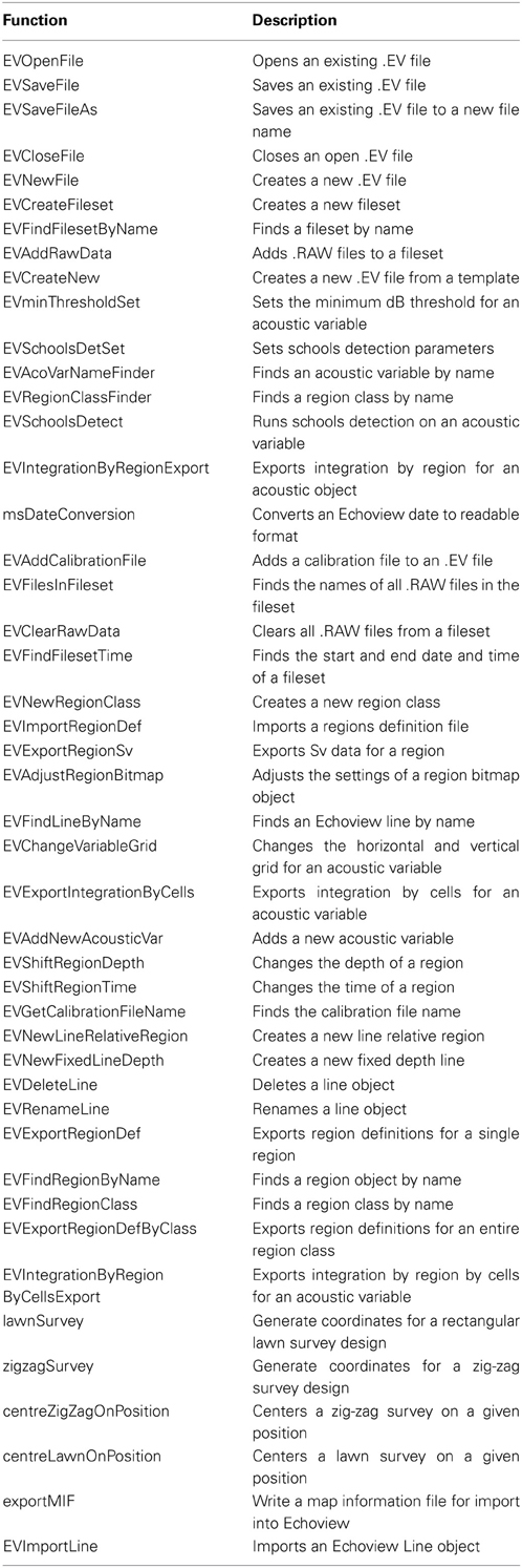
Table 1. Functions available in EchoviewR.

Examples

Here we present two examples using EchoviewR: (1) krill biomass estimation, and (2) krill swarm detection and classification. The purpose of these examples is to demonstrate that these analyses can be run automatically using EchoviewR and to show how Echoview output can be seamlessly linked to analyses carried out using R. Both examples assume that the reader is familiar with Echoview and are not intended to be a tutorial on Echoview. It is also assumed that the reader is familiar with R and programming concepts such as for loops.

The data are a subset of the EK60 split-beam data collected during the Krill Acoustics and Oceanography Survey (KAOS) carried out from RV Aurora Australis. The KAOS survey was undertaken in January–March 2003 off North Eastern Antarctica. Data from 38, 120, and 200 kHz were written to RAW files. For clarity in the worked examples, we have used the 38 and 120 kHz data because these frequencies are the most useful for detecting and identifying the example species, Antarctic krill.

To demonstrate that biomass estimation and swarm detection can be automatically run on multiple transects where the data are too large to practically read in to Echoview at once, as is the case for most acoustic surveys, segments of six KAOS transects are provided and each 10–20 km transect segment is processed separately (Figure 1).

FIGURE 1

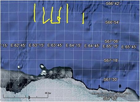
Figure 1. Map showing location of 6 the example transects in yellow. Map created using Google Earth 7.1.2.2041.

Both these examples have been tested using R Studio and 0.98.932 and Echoview 6.1.32.26088. The data to run these examples are available at the Australian Antarctic Division Data Centre [doi: 10.4225/15/54CF081FB955F]. An example of the data flow for the template used in this example is available as Figure S1 in the Supplementary Material.

Before running each example some pre-processing is demonstrated to get the data in to a convenient format for analyzing each transect in a separate .EV file. In this pre-processing phase, the six transects are imported separately into Echoview and the following tasks are performed:

1. Create a new .EV file for the transect using the Echoview template file;

2. Import the EK60 .RAW data files for that transect;

3. Add an Echoview.ecs calibration file;

4. Import .evr region definitions files to remove off effort data;

5. Import a seabed exclusion line (lineKAOS .evl);

6. Close and save the file and repeat for remaining transects.

These steps and the code to run them are demonstrated in the “Read data using the R package EchoviewR to control Echoview via COM” pdf vignette that is available with the Supplementary Material. Pre-processing must take place before examples 1 and 2 are run.

Example 1—Krill Biomass Estimation

Automated biomass estimation of krill is demonstrated by processing the six transects separately in Echoview and exporting the data into R for density and biomass calculation. For each transect, the following steps are taken in Echoview:

1. Open the transect's .EV file.

2. Set the grid for 38 and 120 kHz noise removed values to 50 ping * 5 m depth.

3. Export integration by cells for 38 and 120 kHz noise removed values.

This produces two .csv files for each transect, one containing 38 kHz and one containing 120 kHz integrated data (i.e., a mean volume backscattering strength value for each cell. Then, the following steps are taken in R.

1. Import the 38 and 120 kHz files for the transect.

2. Remove no data values (set -999 and 999 dB as NA) and depths <0.

3. Calculate the krill difference window of 120–38 kHz for each integration cell using the following formula:

$△S{v}_{ij}=S{v}_{{120}_{ij}}-S{v}_{{38}_{ij}}$

where Sv_120ij = mean 120 kHz backscattering strength for cell at interval j at depth i and Sv_38ij = mean 38 kHz backscattering strength for cell at interval j at depth i.

4. Apply the dB difference technique (e.g., Watkins and Brierley, 2002) by setting Sv_120ij values outside the survey-specific dB difference range of 1.04 > = ΔSv_ij < = 14.75 dB to NA as these windows are unlikely to contain krill.

5. Convert the backscattering strength, Sv_120ij for each cell to linear scale, Sv_120ij (Echoview uses a log scale by default):

$s{v}_{ij}={10}^{\frac{S{v}_{ij}}{10}}$

6. Calculate mean volume backscattering strength (MVBS) across all depths for each 50 ping integration interval using the following formula:

$MVB{S}_j=10{\log }_{10}\frac{1}{n_j}{\displaystyle \sum _{i=0}^{n_j}s{v}_{{120}_{ij}}}$

where j = integration interval, n = maximum depth within integration interval j and Sv_120ij = backscattering strength at 120 kHz for interval j at depth i.

7. Calculate estimates of krill density, $\widehat{p}$_j, for each integration interval:

${\widehat{p}}_j=n_j^{\ast }{10}^{\left\{\frac{MVB{S}_j-TS}{10}\right\}}$

where n_j = maximum depth of integration interval j, MVBS_j = mean volume backscattering strength for interval j as calculated above and TS = target strength for 1 kg of krill at 120 kHz.

8. Calculate the overall transect density, $\widehat{p}$_k for transect k:

${\widehat{p}}_k=\frac{1}{s_k}{\displaystyle \sum _{j=1}^{s_k}{\widehat{p}}_j}$

where j = integration interval, k = transect and s_k = number of integration intervals within transect k.

9. The full survey density is then estimated using the Jolly and Hampton (1990) method, which uses the weighted density of each transect by length to calculate total survey density. Note that the formula has been modified to remove stratum as no strata were used in the KAOS example survey design:

$\widehat{p}=w_k{\widehat{p}}_k$

where k = transect, ${\text{w}}_k=\frac{L_k}{L}$, L_k = length of transect k in km, L = length of all survey transects in km and $\widehat{p}$_k = estimated density for transect k.

10. The full survey biomass estimate, $\widehat{b}$, is then calculated by multiplying the weighted survey density by survey area:

$\widehat{b}=\widehat{p}A$

where $\widehat{p}$ = estimated survey biomass and A = survey area in km².

Both the Echoview and R components above are run within loops to allow each transect to be run separately. This is done to demonstrate how looping over transects or days of a large survey is possible, rather than manually loading and processing each set of files. The EchoviewR and R code for the above analysis is shown in the “Biomass estimation using the R package EchoviewR to control Echoview via COM” pdf vignette that is available with the Supplementary Material. Table 2 shows the estimated density, length and biomass for the sample transects and survey area.

TABLE 2

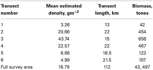
Table 2. Estimated transect krill areal density and survey biomass for the six example transects.

Example 1 has demonstrated the use of EchoviewR to automatically process and extract data by transect from Echoview. Krill density and biomass are then calculated in R using the extracted .csv files.

Example 2—Swarm Detection and Classification

Automated swarm detection and classification of krill aggregations is demonstrated here using EchoviewR. The code for this example is available in the “Schools detection using the R package EchoviewR to control Echoview via COM” pdf vignette file available with the Supplementary Material. Each transect is processed separately to demonstrate how a full survey can be processed automatically using loops. Schools detection is run in Echoview and then detected aggregations are classified and clustered in R. The following steps are undertaken in Echoview using EchoviewR:

1. Open the transect's .EV file.

2. Run schools detection on the variable 120 7x7 convolution, assigning all detected schools to the region class “aggregations.”

3. Export 120 and 38 kHz data for regions of class “aggregations” to a .csv file using the EVIntegrationByRegionExport function. This exports a single mean Sv for each aggregation.

In this example, all detected aggregations are exported. However, it is also possible to export only aggregations classified as krill using the 120-38 aggregation dB difference filter variable included in the template. The filter sets the Krill aggregations data to NULL if the 120-38 aggregation dB difference value for that cell is outside the [1.04, 14.75] dB difference window for the KAOS survey.

The exported aggregations can now be classified and clustered in R. Each transect is run separately using a loop:

1. Import the 120 and 38 kHz export by regions files.

2. Remove null values (-999).

3. Calculate the 120–38 kHz difference window and subset data to only include difference values between [1.04, 14.75].

4. If no aggregations were classified as krill, exit here and move to next transect.

5. If krill aggregations are found, run cluster analysis using the ClusterSim library using selected metrics.

6. Print a summary table of the number of aggregations assigned to each identified cluster. Table 3 shows the number of krill swarms identified and the number of clusters detected for each transect.

TABLE 3

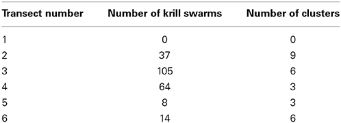
Table 3. Number of unique krill aggregation clusters identified for each transect.

This example has demonstrated how school detection, data export and cluster analysis can be run automatically for an entire acoustic survey.

Discussion and Future Directions

EchoviewR is a free interface between R and Echoview that provides automated acoustic data processing. It drastically decreases manual processing time and reduces subjectivity by providing an easy way to implement exactly the same method across surveys. This package enables reproducible methodology, which is a vital part of the scientific method. We have given examples of automated krill biomass estimation and school detection using EchoviewR that demonstrate the use of the package on a subset of the KAOS survey. This method can easily be extended to run a full survey by transect, day or any other subset required.

There are a number of limitations to the package. Currently it is only available for use for single and split beam echo sounder data. EchoviewR is also unable to handle removal of noise and false bottom effects, which must be completed prior to using the package. Not all functions in Echoview are currently available using EchoviewR, however any COM functionality in Echoview can be implemented in R. The COM hierarchy help page is a useful starting point for those wishing to add extra functions.

EchoviewR is accessible as free software from the EchoviewR GitHub repository (https://github.com/lisamarieharrison/EchoviewR) and is readily available for community development. An important next step is the implementation of false bottom and noise removal using EchoviewR, and it is our hope that the acoustic community will take the tools that we are providing and extend the package to include the functionality that they require. We also underline that the methods described here are generic, and hope the work can inspire the implementation of scripting interface in other acoustic processing software.

Conflict of Interest Statement

The authors declare that the research was conducted in the absence of any commercial or financial relationships that could be construed as a potential conflict of interest.

Acknowledgments

We would like to thank Echoview for their support of this project. This research is a contribution to Australian Antarctic Division science programme Project 4104 and project 4102. MC is funded by Australian Research Council grant FS11020005. LH is funded by a Macquarie University Research Excellence Scholarship.

Supplementary Material

The Supplementary Material for this article can be found online at: http://www.frontiersin.org/journal/10.3389/fmars.2015.00015/abstract

Figure S1. Screenshot of the Echoview data flow used for the examples. Template made using Echoview 6.0.

References

Benoit-Bird, K. J., Battaile, B. C., Heppell, S. A., Hoover, B., Irons, D., Jones, N., et al. (2013). Prey patch patterns predict habitat use by top marine predators with diverse foraging strategies. PLoS ONE 8:e53348. doi: 10.1371/journal.pone.0053348

Pubmed Abstract | Pubmed Full Text | CrossRef Full Text | Google Scholar

Bivand, R., and Lewin-Koh, N. (2014). maptools: Tools for Reading and Handling Spatial Objects. R Package Version 0.8-29. Available online at: http://CRAN.R-project.org/package=maptools

Bivand, R., and Rundel, C. (2014). rgeos: Interface to Geometry Engine - Open Source (GEOS). R package version 0.3-4. Available online at: http://CRAN.R-project.org/package=rgeos

Brierley, A. S., Fernandes, P. G., Brandon, M. A., Armstrong, F., Millard, N. W., McPhail, S. D., et al. (2002). Antarctic krill under sea ice: elevated abundance in a narrow band just south of ice edge. Science 295, 1890–1892. doi: 10.1126/science.1068574

Pubmed Abstract | Pubmed Full Text | CrossRef Full Text | Google Scholar

Brown, C. J., Hewer, A. J., Meadows, W. J., Limpenny, D. S., Cooper, K. M., and Rees, H. L. (2004). Mapping seabed biotopes at hastings shingle bank, eastern English Channel. Part 1. Assessment using sidescan sonar. J. Mar. Biol. Ass. U.K. 84, 481–488. doi: 10.1017/S002531540400949Xh

CrossRef Full Text | Google Scholar

De Robertis, A., and Higginbottom, I. (2007). A post-processing technique to estimate the signal-to-noise ratio and remove echosounder background noise. ICES. J. Mar. Sci. 64, 1282–1291. doi: 10.1093/icesjms/fsm112

CrossRef Full Text | Google Scholar

Gerlotto, F., Soria, M., and Fréon, P. (1999). From two dimensions to three: the use of multibeam sonar for a new approach in fisheries acoustics. Can. J. Fish. Aqua. Sci. 56, 6–12. doi: 10.1139/cjfas-56-1-6

CrossRef Full Text | Google Scholar

Grolemund, G., and Wickham, H. (2011). Dates and times made easy with lubridate. J. Stat. Softw. 40, 1–25.

Google Scholar

Guihen, D., Fielding, S., Murphy, E. J., Heywood, K. J., and Griffiths, G. (2014). An assessment of the use of ocean gliders to undertake acoustic measurements of zooplankton: the distribution and density of Antarctic krill (Euphausia superba) in the Weddell Sea. Limnol. Oceanogr. 12, 373–389. doi: 10.4319/lom.2014.12.373

CrossRef Full Text | Google Scholar

Hijmans, R. J. (2014). geosphere: Spherical Trigonometry. R Package Version 1.3-8. Available online at: http://CRAN.R-project.org/package=geosphere

Johansen, G. O., Godø, O. R., Skogen, M. D., and Torkelsen, T. (2009). Using acoustic technology to improve the modelling of the transportation and distribution of juvenile gadoids in the Barents Sea. ICES. J. Mar. Sci. 66, 1048–1054. doi: 10.1093/icesjms/fsp081

CrossRef Full Text | Google Scholar

Jolly, G., and Hampton, I. (1990). A stratified random transect design for acoustic surveys of fish stocks. Can. J. Fish. Aquat. Sci. 47, 1282–1291. doi: 10.1139/f90-147

CrossRef Full Text | Google Scholar

McGonigle, C., Brown, C., Quinn, R., and Grabowski, J. (2009). Evaluation of image-based multibeam sonar backscatter classification for benthic habitat discrimination and mapping at Stanton Banks, UK. Estuar. Coast. Shelf Sci. 81, 423–437. doi: 10.1016/j.ecss.2008.11.017

CrossRef Full Text | Google Scholar

Myriax. (2015). Echoview. Hobart, TAS. Available online at: http://www.echoview.com/

Pebesma, E. J., and Bivand, R. S. (2005). Classes and methods for spatial data in R. R News 5 (2), Available online at: http://cran.r-project.org/doc/Rnews/

R Development Core Team. (2014). R: A Language and Environment for Statistical Computing. Vienna: R Foundation for Statistical Computing.

Rstudio. (2014). RStudio: Integrated Development Environment for R (version 0.98.932). Boston, MA. Available online at: http://www.rstudio.com/

Van Walree, P. A., Têgowski, J., Laban, C., and Simons, D. G. (2005). Acoustic seafloor discrimination with echo shape parameters: a comparison with the ground truth. Cont. Shelf Res. 25, 2273–2293. doi: 10.1016/j.csr.2005.09.002

CrossRef Full Text | Google Scholar

Watkins, J. L., and Brierley, A. S. (2002). Verification of the acoustic techniques used to identify Antarctic krill. ICES. J. Mar. Sci. 59, 1326–1336. doi: 10.1006/jmsc.2002.1309

CrossRef Full Text | Google Scholar

Weber, T. C., Jerram, K., and Mayer, L. (2014). “Acoustic sensing of gas seeps in the deep ocean with split-beam echosounders,” in Proceedings of Meetings on Acoustics (Edinburgh, EB), 17.

Google Scholar