Scaling Precipitation Input to Spatially Distributed Hydrological Models by Measured Snow Distribution

1. Introduction

The spatial distribution of snow depth can vary on scales of a few meters and from winter to winter. Different precipitation patterns, redistribution by wind, temperature and solar radiation strongly control snow distribution. The seasonal snow cover in alpine terrain accumulates and stores a large amount of water and has a major influence on the release and availability of water throughout the year. The water stored in snow is essential for hydro-power (Schaefli et al., 2007), water supply and recreational activities (Koenig and Abegg, 1997). Additionally, the development of flora and fauna in the alpine and lower elevated areas is influenced by the snow cover (Wipf et al., 2009) and the formation of avalanches is substantially influenced by the spatial and temporal distribution of the snow cover (Schweizer et al., 2003).

Using numerical models, snow distribution in alpine terrain can be simulated (Liston and Sturm, 1998; Gauer, 2001; Winstral et al., 2002; Vionnet et al., 2014). Simulations can be used to understand hydrological processes (Comola et al., 2015), for fore- and now-casting (Lehning et al., 1999; Bellaire et al., 2011) or the assessment of climate change (Bavay et al., 2009). The spatially distributed, physics-based model Alpine3D is suitable for simulations of snow in steep, alpine terrain (Lehning et al., 2006, 2008). It accounts for the most relevant processes leading to snow accumulation, ablation, metamorphism and the energy exchanges with soil, vegetation and the atmosphere. As simulations may become computationally expensive, not all processes can be explicitly accounted for in a simulation. Effects caused by wind, such as snow transport and preferential deposition, can be included (Lehning et al., 2008), but the computational demand increases dramatically. These effects are therefore often neglected, leading to errors in snow distribution. Also a detailed representation of the energy fluxes (Michlmayr et al., 2008) limits the applicability of large-scale simulations with high spatial resolution. Uncertainties in and lack of measurements of meteorological observations, which are usually used as input, contribute to errors in the simulation of snow distribution (Schölgl et al., 2016) and the measurements are often not representative for the vicinity of the automatic weather station (AWS) (Grünewald and Lehning, 2015).

Various simple methods to allocate precipitation to account for wind drift have been tested in previous studies. Most of them use topographic features such as elevation, slope, aspect and/or curvature (Schuler et al., 2007; Huss et al., 2008; Magnusson et al., 2014). More complex parameters are also calculated, e.g., topographic openness (Hanzer et al., 2016). The most successful topographic parameter is the Winstral redistribution parameter (Winstral et al., 2002, 2013), which has been shown to give good results even in fairly difficult conditions if at least the mean wind direction is known (Schirmer et al., 2011).

Recent advances in remote sensing techniques enable us to acquire information about the earth surface with high vertical accuracy and high spatial resolution and allow new quantitative insight in snow distribution (Trujillo et al., 2007; Deems et al., 2013). Terrestrial laser scanning (TLS) can be used to measure the snow surface continually (Grünewald et al., 2010; Deems et al., 2013) and with very high accuracy (less than 20 cm error on average Prokop et al., 2008). However, this method is labor intensive and limited to small areas only (Bühler et al., 2013). Airborne mounted scanning devices are well suited to gather information about the spatial distribution and thickness of the snow cover for large areas. Using an opto-electric scanner for large areas is cheaper than using laser scanning (Bühler et al., 2013). With an opto-electric scanner, stereo images are acquired and can be combined to a digital surface model (DSM) (Kresse and Danko, 2012; Bühler et al., 2015). If snow free DSMs are subtracted from DSMs with snow covered areas, maps of spatial snow distribution can be generated. Such maps of snow depth, temporally close to the maximum seasonal snow depth, have been acquired in recent years for the region of Davos, Switzerland (Bühler et al., 2012, 2013). Such maps can be used for validation purposes of the performance of numerical models. They also offer the potential to be included as model input to improve the model performance (e.g., Revuelto et al., 2016). They used TLS data to adjust snow depths on dates where TLS scans were available in simulations throughout different winters. This method allows to correct the snow depth at time steps where TLS information is available and it was shown to improve the simulation of snow depth. However, the method either requires multiple TLS scans per winter, or it will only provide an accurate snow depth distribution on or directly after the TLS scan and during melting periods. During snow accumulation periods, TLS information is essential to improve simulation performance. Furthermore, snowpack layering and snow microstructure may not be well represented when simulated snow depth deviates from actual snow depth for extended periods of time.

In this work, a simple method of precipitation scaling using remote sensing datasets is presented. The method aims to achieve an accurate simulation of seasonal snow cover with one simulation run only. A characteristic of the model is that it distinguishes between different precipitation patterns depending on the precipitation phase. A comparison of the scaling methods with non-scaling methods and an iterative scaling approach is made to quantify the gain in accuracy based on the scaling. Problems and limitations of the methods are investigated and described.

2. Methods

2.1. Site Description

To investigate the potential of precipitation scaling the area around the town Davos, Switzerland was chosen. For this area, several airborne digital sensor (ADS) remote sensing datasets of seasonal snow distribution are available (Bühler et al., 2015). This area has been the basis for numerous research projects and numerical simulations have been run in this area for various applications (e.g., Zappa et al., 2003; Bavay et al., 2009; Mott et al., 2011). The simulation domain covers an area of 21.5 × 21.5 km centered around the Dischma valley south-east of Davos (cf. Figure 1). The mean elevation of the domain is 2256 m.a.s.l. with a minimum elevation of 1255 m.a.s.l. and the highest peak at 3218 m.a.s.l. The lower areas, below ~1800 m.a.s.l., are mostly covered by forest (13.2% of the domain) and infrastructure and buildings of Davos (1.3% of the domain). The higher areas are mostly covered by alpine meadow (21.8% of the domain), changing into rocky and glacial areas in the highest elevations of the domain. The glacial areas cover 2.9% of the domain. The most dominant precipitation pattern is determined by the elevation gradient. Precipitation amounts at the Weissfluhjoch are about twice as high as in Davos (Wever, 2015).

FIGURE 1

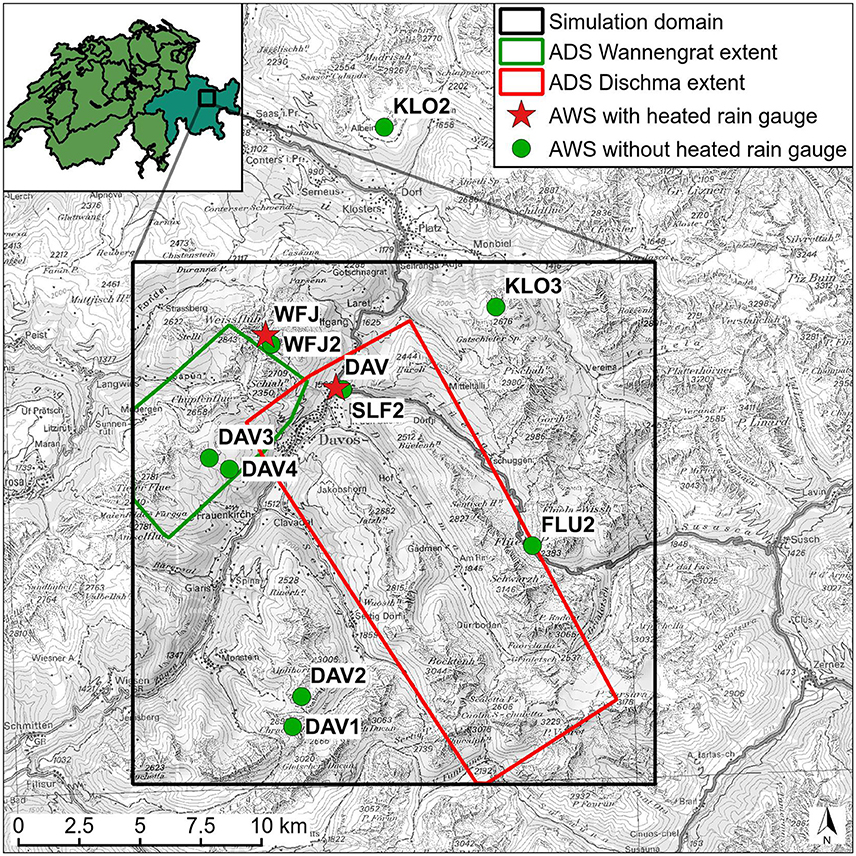
Figure 1. Overview of the simulation domain in the area of Davos, Switzerland (black frame), the ADS (airborne digital sensor) Wannengrat extent (green frame) and the ADS Dischma extent (red frame). The AWSs used for Alpine3D input with (red stars) and without heated rain gauge (green dots). Maps reproduced by permission of swisstopo (JA100118).

Several meteorological stations are located within the simulation domain (cf. Figure 1). Most of them belong to the Intercantonal Measurement and Information System, a permanently operating network for avalanche warning (Lehning et al., 1999). These stations measure general meteorological parameters such as air, soil and snow temperatures, wind speed and direction, relative humidity and snow depth and reflected short-wave radiation but not precipitation. A meteorological station at the Weissfluhjoch (WFJ, 2540 m.a.s.l.) and one in Davos (DAV, 1596 m.a.s.l.), belonging to the SwissMetNet from MeteoSwiss (Heimo et al., 2007) are equipped with heated rain gauges, providing information about precipitation at different elevations. These stations are also equipped with sensors to measure incoming short-wave radiation and incoming long-wave radiation. Figure 1 gives an overview of the location and extent of the simulation domain and ADS extents, including the locations and code names of the AWS sites.

2.2. Remote Sensing Data

The maps of measured spatial snow depth distribution were generated using information acquired by the ADS technology (Bühler et al., 2015). The opto-electric line scanners ADS80 and ADS100 from Leica Geosystems were used to acquire summer and winter stereo images for different years over the Dischma and Wannengrat area near Davos (cf. Figure 1). The ADS dataset covering the Wannengrat area (~3.5 × 7.5 km) and the Dischma area (~7 × 17 km) are merged and handled as one dataset. The acquired images were processed to digital surface models (DSM) for summer and winter (Bühler et al., 2012). Subtracting the winter DSM from the summer DSM provides to maps of snow depth. The resolution of the final snow depth maps is 2 m with an average vertical accuracy of ±30 cm (Bühler et al., 2015).

To use the ADS data for scaling, it was resampled to a 100 m resolution by averaging when more than 50% of the grid points contained data. If more than 50% of the grid points contained no data, also the resampled grid point was set to no data. Snow depth in areas covered with forest, scrub, buildings and water bodies can not be determined using ADS technology (Bühler et al., 2015) and are therefore masked out from the datasets. ADS datasets from 20 March 2012, 15 April 2013 and 17 April 2014 were used in this study. All snow depth maps were calculated using a summer DSM from 3 September 2013. Figure 2 shows the ADS data for 20 March 2012 at 100 m resolution.

FIGURE 2

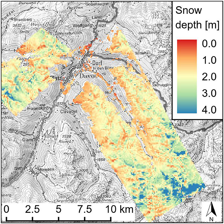
Figure 2. ADS snow depth map from 20 March 2012 resampled at 100 m resolution. Legend shows snow depth [m] and correspond to the 2–98 cumulative percentage of data. Map reproduced by permission of swisstopo (JA100118).

2.3. Numerical Modeling

2.3.1. Models

Alpine3D is an Open Source model of mountain surface processes with a special focus on snow cover. It has been designed for hydrological, meteorological and avalanche warning applications in steep, alpine terrain (Lehning et al., 2006). It consists of several modules simulating various processes: a module for snow transport (Lehning et al., 2008; Groot Zwaaftink et al., 2011), a module to simulate the radiation fields in complex terrain (Michlmayr et al., 2008; Helbig, 2009) or a module to provide runoff data in order to couple it with an hydrological routing scheme (Gallice et al., 2016). As the snow transport module requires the computation of 3D wind fields and comes at a very high computational cost, it has not been used for the simulations in this work. Similarly, the radiation fields have been treated by a simpler module that accounts for shading effects, atmospheric attenuation and a simplified representation of the radiation reflected by the surrounding terrain based on a view factors approach (similarly to Anslow et al., 2008; Endrizzi et al., 2014).

At its core, Alpine3D is a distributed version of the SNOWPACK model (Bartelt and Lehning, 2002; Lehning et al., 2002a,b): 1D simulations are run for all grid points in the simulation domain and then processed by the other modules. The SNOWPACK model describes physical processes in and between soil, snow and vegetation and the atmospheric boundary layer with high accuracy (Wever et al., 2014, 2015). It can for example simulate the deposition and resublimation of surface hoar, the shortwave penetration into the snow cover and local phase changes. It uses a variable number of layers with a typical thickness of less than 2 cm and gives an overall reliable representation of the local snow mass balance if accurate forcing data is available.

The meteorological forcing data are taken from AWS. These raw data are filtered and preprocessed (more in Section 2.3.2) using the Open Source MeteoIO library (Bavay and Egger, 2014) before entering the core of the model. Since the MeteoIO library computes the distributed meteorological forcing, the precipitation scaling method presented here has been directly implemented into MeteoIO as another spatial interpolation algorithm. Alpine3D is used as a framework here to determine the potential of precipitation input scaling to improve the accuracy of spatial snow distribution in numerical models.

2.3.2. Input Data

For the simulations presented here, all input data are taken from AWSs and interpolated on the simulation domain. The two SwissMetNet stations are used for incoming short-wave radiation and incoming long-wave radiation. Precipitation input is chosen depending on the simulation and is explained later. The other parameters are interpolated from all AWS. Depending on the number of input sources, different interpolation methods are applied to distribute the observations on the domain. If none or only one source is available, a default or constant value (CST) or a predefined lapse rate (CST-LAPSE) are used to generate distributed input. Additionally, if at least two sources are available, a lapse rate can be calculated (LAPSE). If more than two sources are available, a combination of inverse distance weighting and a lapse rate (IDW-LAPSE) can be applied for interpolation (Bavay and Egger, 2014). For most input data except precipitation IDW-LAPSE is used for interpolation. For precipitation, generally only few inputs are available and IDW-LAPSE is rarely used.

In this study, we used two different interpolation methods for precipitation. For simulations with two rain gauges we interpolated with lapse rate only. For simulations with more than two precipitation inputs, we used a combination of inverse distance weighting and lapse rate (Bavay and Egger, 2014). For the simulations presented here two different precipitation input sources are used. Simulations using hourly observations from two heated rain gauges, interpolated on the simulation domain are called [PSUM], as they use precipitation sums as input. Simulations where precipitation is generated from snow depth changes measured by AWSs (Lehning et al., 1999; Wever et al., 2015) are called [HS]. Using SNOWPACK, a precipitation rate corresponding to the observed change in snow depth is calculated, considering snow density and settling. In total 9 AWS are used to provide precipitation input. The [PSUM] and [HS] simulations are traditional, non-scaling methods used as reference to compare to the scaling methods and serve as the baseline precipitation field for the scaling methods. The interpolation methods for the different input sources are summarized in Table 1.

TABLE 1

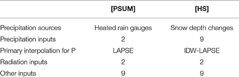
Table 1. Overview of the inputs and interpolation methods used in the simulations.

When using the heated rain gauges as precipitation input, the data from winter 2012/13 and 2013/14 are corrected for undercatch according to Goodison et al. (1998). Unusual meteorological circumstances in winter 2011/12 with strong winds and associated increased snow transport, led to a situation where undercatch correction was not necessary in order to accurately represent the snow depth at the WFJ and DAV measurement sites (Wever et al., 2015), and therefore, the undercatch correction was not applied for any simulations in this winter.

2.3.3. Direct Scaling Method

The direct scaling method is designed to scale precipitation input with one simulation run only and can be applied to any precipitation input. Here the [PSUM] and [HS] inputs are used to test direct scaling. First, precipitation is interpolated using LAPSE ([PSUM]) or IDW-LAPSE ([HS]) to provide the initial guess of the precipitation field over the total simulation domain. In a second step, the precipitation is redistributed using the snow depth information from the ADS data according to Equation (1):

$\begin{array}{ll}{P}_{i,t}=\frac{P_{avg,t}}{H{S}_{avg}}·H{S}_i& (1)\end{array}$

P_{i, t} is the amount of scaled precipitation distributed on a grid point i at time t. P_{avg, t} is the spatial average interpolated precipitation at time t, HS_avg is the average snow depth of the ADS data for the same domain and HS_i is the ADS snow depth at grid point i. The redistribution of precipitation is done only for grid points where ADS information is available. P_{avg, t} is calculated only for the area where ADS information is available to guarantee mass conservation. ADS information (e.g., HS_avg, HS_i) is always taken from one of the three ADS datasets available, depending on the simulated winter. This simple scaling assumes that the spatial precipitation correction factor is time-invariant. This scaling approach leads to a separation between the total precipitation input and scaling the distribution. The total precipitation mass interpolated on the domain is strictly conserved while being redistributed and scaled onto the domain.

To account for the different precipitation patterns of solid and liquid precipitation, the precipitation is redistributed and scaled only when the air temperature (TA) on the grid cell is below a certain threshold value. Therefore, TA is interpolated over the simulation domain using IDW-LAPSE. If the air temperature at a grid point is above this threshold, only liquid precipitation is assumed and no scaling is applied, assuming the interpolation is already a good approximation for rainfall patterns. If the air temperature is below the threshold, a distribution according to Equation (1) is applied. The threshold for all simulations conducted in this study is set to 1.2°C. Figure 3 schematically shows the structure of the scaling method. The simulations scaling [PSUM] input are called [PAT] (from PSUM-ADS-Threshold), the simulation scaling [HS] input are called [HAT] (from HS-ADS-Threshold).

FIGURE 3

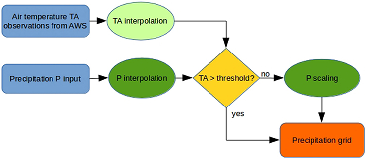
Figure 3. Flow chart of the direct scaling method. An air temperature (TA) and a precipitation (P) field are generated for every time step from local time series at AWSs. Depending on the air temperature at each grid point, a decision is made if the interpolated precipitation is scaled according to the ADS data or not.

2.3.4. Iterative Scaling Method

The results from an initial scaling may be improved considerably by an additional iteration step, which takes into account the deviation between simulated and measured snow depth after a first model run. The additional computational costs may be justified for applications were a precise snow depth distribution is important as well as simultaneously maintaining a correct spatial and timely simulation of individual snow fall events (e.g., snow avalanche prediction). Here, we also investigate the improvement in snow depth distribution by an iterative scaling approach [ALS2] (from Airborne Landscape Scans with 2 simulation runs), compared to direct scaling.

For [ALS2] simulations precipitation grids are calculated for each time step and fed into the model by assessing the precipitation on each grid point proportional to the ratio between the average snow depth in the ADS data at the elevation of a rain gauge (cf. Equation 2).

$\begin{array}{ll}{P}_{i,t}=\frac{P_{DAV,t}}{H{S}_{1595}}·H{S}_i& (2)\end{array}$

P_{i, t} is the amount of precipitation allocated to grid point i at time step t, P_{DAV, t} is the measured amount of precipitation at time t at station Davos (DAV), HS₁₅₉₅ is the average snow depth of all grid points at 1595 m.a.s.l. (± 10 m), which is the elevation of the station Davos and HS_i is the ADS snow depth on grid point i. It is assumed that the average snow depth at this elevation is represented by the precipitation measured at DAV.

From the resulting snow distribution at the date where the ADS dataset was acquired, a correction grid is calculated (cf. Equation 3). With this correction grid, all precipitation input grids from the first simulation are corrected (cf. Equation 4). The simulation is re-run using the corrected precipitation input grids.

$\begin{array}{rcll}{f}_{c,i}& =& \frac{H{S}_i}{H{S}_{ALS,i}}& (3)\end{array}$

$\begin{array}{rcll}{P}_{2,i,t}& =& P_{i,t}·f_{c,i}& (4)\end{array}$

P_{2, i, t} is the corrected precipitation for grid point i at time t. P_{i, t} is the original precipitation field used in the first simulation run (cf. Equation 2), f_{c, i} is the correction factor for grid point i, HS_i is the ADS snow depth and HS_{ALS, i} is the snow depth resulting from the first run at grid point i. This iterative method requires substantially more effort and model adjustment because simulations have to be carried out twice.

2.4. Simulation Setups

For the two precipitation sources described above, non-scaling simulations ([PSUM] and [HS]) were run. For the same precipitation inputs used in [PSUM] and [HS], simulations were run using the direct scaling, which results in the experiments [PAT] and [HAT]. [PAT] is the scaled simulation of [PSUM] and [HAT] is the scaled simulation of [HS]. Additionally, simulations for the iterative scaling method [ALS2] were conducted. For all simulation setups only the precipitation input was varied. All other inputs remained unchanged and were equal for any simulation. Simulations were conducted for the winters 2011/12, 2012/13, and 2013/14. ADS data from March 2012, April 2013 and 2014 were used for scaling. Simulations were run from August to July. To assess the potential of inter-annual scaling, the direct scaling simulations were run using all ADS datasets to scale all simulated winters e.g., winter 2011/12 was simulated using the corresponding ADS dataset 2012 for scaling, but also the datasets from 2013 and 2014. The same was done for winter 2012/13 and 2013/14. This inter-annual scaling can be considered as a cross-validation variant but is also of practical interest as it should show, how snow distribution acquired with quite some effort in a particular year can then be used in other years.

2.5. Data Analysis

The analysis of the simulation results was done for the dates of ADS data acquisitions. From simulated snow depths and ADS data, relative and absolute errors are calculated for each grid point and compared. The absolute errors are calculated according to Equation (5) and the relative errors according to Equation (6).

$\begin{array}{rcll}\Delta HS& =& H{S}_{sim}-H{S}_{ADS}\left[m\right]& (5)\end{array}$

$\begin{array}{rcll}\delta HS& =& \frac{H{S}_{sim}-H{S}_{ADS}}{H{S}_{ADS}+0.0001m}\left[-\right]& (6)\end{array}$

ΔHS is the absolute error in snow depth, δHS is the relative error in snow depth, HS_sim is the snow depth simulated with Alpine3D at the same date where the ADS data is acquired and HS_ADS is the snow depth information from the 100 m ADS dataset. To avoid divisions by zero, 0.0001 m of snow depth where added to the ADS snow depth when calculating the relative errors. Additionally relative errors larger than 5 and smaller than −5 are classified as outliers and excluded from data analysis. At small snow depths, the relative error is highly sensitive and small absolute errors in snow depth can lead to very high relative errors. Nevertheless, the relative error is helpful to identify errors in snow depth simulations in complex terrain on the small scale, e.g., along ridges or depressions. Here we concentrate on the absolute error and maps of absolute errors of different simulations are shown. Maps of relative errors can be found in the Supplementary Material.

3. Results and Discussion

3.1. Non-scaling Simulations

In non-scaling [PSUM] simulation for winter 2011/12 the local snow depth is over- and underestimated but maximum errors remain smaller than ±2 m. The strongest underestimations occurred in the highest elevations in the south-east of the simulation domain (cf. Figures 4A,B). This area is also most distant from the rain gauges. Overestimation occurred at all elevations and mostly in north facing slopes. Distributions of the errors for the winters 2012/13 and 2013/14 are similar (cf. Table 2). Figure 4B shows that small snow depths at low elevations are generally overestimated by the simulation. At higher elevations, underestimations occur almost with the same frequency as overestimations and the error magnitude increases with elevation. The mean absolute error is 0.044 m with a standard deviation of 0.569 m. The mean snow mass is distributed very accurately by the two rain gauges. Given the fact that other studies (e.g., Grünewald and Lehning, 2011) found that two stations generally are not able to accurately represent elevation gradients in a mountain catchment, we consider it a coincidence that these two rain gauges are able to represent the mass distributed in this catchment accurately. A dependency of errors on the aspect of the slopes is present but not very strong. Small snow depths are generally found in south facing slopes whereas the largest snow depths are found in north facing slopes. Results for the winter 2012/13 are similar and summarized in Table 2 and Figure 5. For winter 2013/14 the mean error was 0.174 m and the standard deviation was 0.399 m.

FIGURE 4

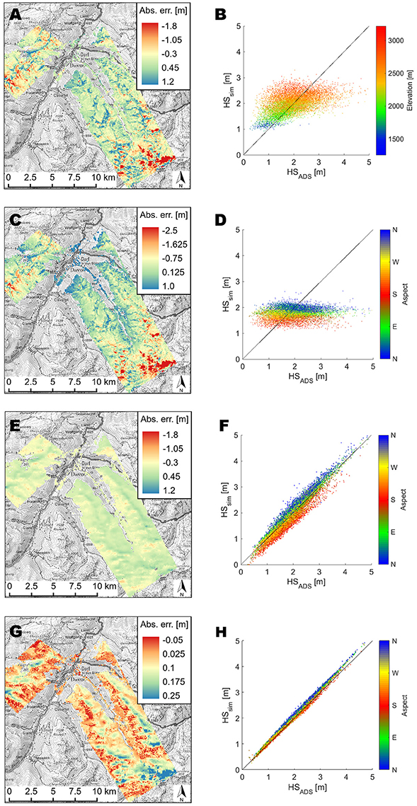
Figure 4. (A,C,D,E,G) Maps of absolute errors in snow depth between simulation results and ADS dataset for 20 March 2012. (B,D,F,H) Scatter plots of simulated against ADS snow depth for 20 March 2012. The plots show [PSUM], [HS], [PAT], and [ALS2] simulation results from winter 2011/12. The range of the absolute errors show the 2–98 cumulative percentage of data for [PSUM], [HS], and [ALS2]. For [PAT] the data range is identical to the [PSUM] data range. Colors in scatter plots correspon to elevation in [PSUM] and aspect of the grid point for others. Maps reproduced by permission of swisstopo (JA100118).

TABLE 2

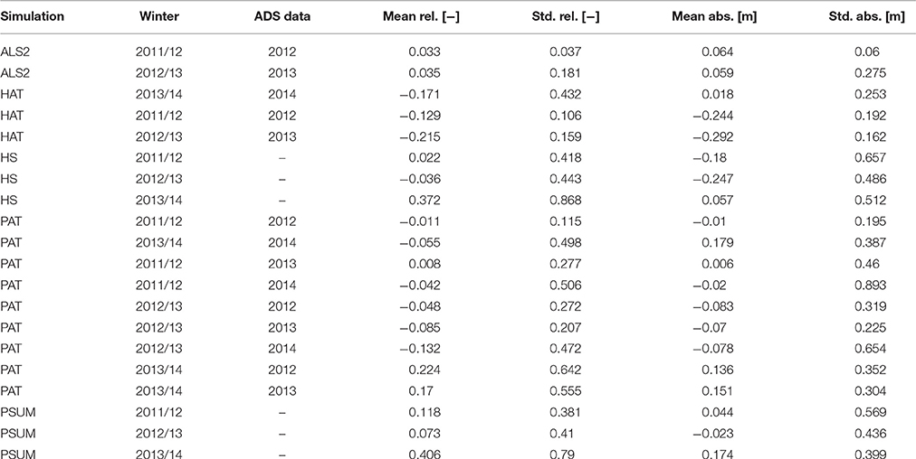
Table 2. Overview on the statistics of the relative (rel) and absolute (abs) errors [mean and standard deviation (std)] for all simulations conducted.

FIGURE 5

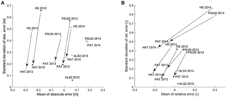
Figure 5. (A) Plot of mean absolute error and standard deviation, (B) Plot of the mean relative error and standard deviation for non-scaling and scaling simulations for the winters 2011/12, 2012/13, and 2013/14. Arrows indicate the effect of the scaling. Simulations from winter 2011/12 are colored in red.

In [HS] simulations, the range of the absolute error is similar to the [PSUM] simulations. Most negative errors in snow depth are present in high alpine terrain and most positive errors occur at lower elevations (cf. Figure 4C). Figure 4D shows the deviation of snow depth from the ADS 2012 dataset for each grid point. It is clear that the range of snow depths of the simulation is limited between 1.5 and 2.5 m, whereas the ADS snow depths vary between 0.5 and more than 4 m. This indicates that an inadequate elevation gradient of precipitation has been calculated from the snow depth stations. Small snow depths at lower elevations are generally overestimated, high snow depths are generally underestimated. The mean absolute error is at -0.18 m with a standard deviation of 0.657 m. The smaller snow depths are generally simulated in south facing slopes whereas the largest snow depths are found in north facing slopes. Results for winter 2012/13 are similar to the ones from winter 2011/12. For winter 2013/14 the absolute mean error was 0.057 m only with a standard deviation of 0.512 m (cf. Table 2).

3.2. Direct scaling

The simulation using the [PAT] scaling approach represents the snow depth on average well (mean absolute error for winter 2011/12 = −0.01 m). Also the standard deviation of the error is rather low at 0.195 m. Small snow depths are generally slightly underestimated whereas large snow depths are slightly overestimated (cf. Figures 4E,F). An over- and underestimation depending on the slopes aspect is visible. The north facing slopes are generally overestimated whereas the snow depths in south facing slopes are underestimated. Results from other winters are similar and are shown in Table 2.

The results of the [HAT] simulation are similar to the [PAT] results, but generally underestimating the snow depths. The mean absolute error is -0.24 m with a standard deviation of 0.19 m for the winter 2011/12. For the winter 2012/13 the mean error was slightly lower and the standard deviation was reduced from 0.486 m to 0.162 m. For the winter 2013/14 the standard deviations were in the same range as for the other winters but with the lowest mean error of 0.018 m.

Comparing the non-scaling simulations to the direct scaling simulations with the same precipitation input (cf. Figure 5A), it can be stated that for any simulation using scaling the standard deviation is strongly reduced. For the winters 2011/12 and 2012/13 it is reduced to less than 0.23 m for all scaling experiments. For the winter 2013/14 for the rain gauge driven simulations no significant reduction in standard deviation of the absolute error results. This is mainly due to rather small snow depths in this winter and an overestimation of the total precipitation in the [PSUM]/[PAT] simulations. This effect becomes visible when considering the change of relative errors (cf. Figure 5B). It can be seen that the standard deviation of the relative errors is significantly reduced. For all simulations, a reduction of total snow depth of about 10 cm is evident for the winters 2011/12 and 2012/13.

3.3. Iterative Scaling

Using the results from the first run to correct the precipitation field, the mean error and standard deviation are reduced remarkably in [ALS2] to a very good representation of snow depth distribution (cf. Figures 4G,H). After the second, iterative simulation run, the snow depths in south facing slopes are generally slightly underestimated whereas in the north facing slopes they are slightly overestimated. The mean absolute error in winter 2011/12 is 0.064 m with a standard deviation of 0.06 m. For winter 2012/13 the mean error is similar with 0.059 m with a standard deviation of 0.12 m (cf. Table 2). For winter 2013/14 no simulation was run.

3.4. Discussion of Scaling Influence

The results of the simulations show that large variations in the results are obtained, depending on the precipitation input chosen and the applied scaling method. The non-scaling methods have the problem that the effective range of snow depths in the domain up to more than 4 m is not correctly represented. They typically occur as a result of local processes (e.g., snow transport) and/or geographical precipitation gradients that are not captured by the interpolation mechanisms.

As only two rain gauges are used in [PSUM] simulations, no IDW is applied and the interpolation cannot account for the climatological north-south gradient in the domain. Therefore, we assume that the interpolation using a lapse rate only is not able to represent the total range of the snow distribution for the simulation domain. As the average error in snow depth is rather small it can also be stated that the precipitation observations do represent the total precipitation well but the correct spatial allocation is missing. The accurate interpolation of total precipitation from two rain gauges also is coincidence since earlier investigations in the catchment (Grünewald and Lehning, 2011, 2015) have shown that individual stations are usually not representative in this type of terrain.

In the [HS] simulations the interpolation is done using IDW-LAPSE. Even though 9 precipitation inputs are interpolated, the range of snow depths was found to be not represented. We hypothesize that this is mainly due to the fact that the measured snow depths by AWSs show limited representativeness for the stations' vicinity (Grünewald and Lehning, 2015) and therefore also the calculated precipitation is not a sufficient input for the whole simulation domain. This shows that the precipitation input needs to be representative for a larger area than only the point where the observation is made. Also the stations are not located at very exposed locations and their data cannot account for the wind blown, shallow snowpack along ridges nor the drift-filled gullies in their vicinity, where generally no station is placed.

The [ALS2] method leads to the best results in terms of spread of the errors (standard deviation = 0.06 m) and a very small mean error of 0.064 m for 2011/12. This is mainly attributed to the fact that there is an iteration, in contrast to the other methods. This makes this method the most reliable one tested in this study, but requires two simulation runs to achieve good results. The small errors still evident in the [ALS2] result from the non-linear settling of the snow cover. A reduction of the precipitation by a factor of 2 does not lead to a reduction of the snow depth by a factor of 2, but a little less. With the adjustment of the precipitation, the settling caused by the snow covers own weight is influenced most. When snow mass is reduced, settling is disproportionately reduced due to missing mass and vice versa, leading to small errors in snow depth simulation. As the iterative approach is independent of direct precipitation measurements, the mean precipitation can be estimated with highest accuracy of all methods tested.

The direct scaling method redistributes the precipitation calculated by the base method [PSUM] or [HS]. Therefore, the influence of the scaling on the mean error is small and depends a lot on the precipitation input. The total precipitation mass allocated by the base method is not influenced and changes in the mean errors occur only due to the redistribution of the precipitation mass to other grid points, which are then influenced differently by temperature, radiation, rain or metamorphism, which all influence settling and lead to a change in snow depth.

For all scaling runs, it is evident that for south facing slopes the snow depth is mostly underestimated whereas it is mostly overestimated in north facing ones. The influence of the aspect on the results will be discussed below.

Looking at the absolute error for the simulations [PSUM] and [PAT] the errors are strongly reduced. The mean error only varies slightly due to the mass conservation in the scaling method but the standard deviation is reduced by a factor of 2.9 from 0.569 m to 0.195 m, leading to errors less than ±1 m overall. The effect of the [HAT] method on the errors is comparable to the [PAT] method. The standard deviation of the absolute error is reduced by a factor of 3.4 to 0.192 m only. The mean error slightly shifts into a more negative area. This shift is mainly due to the redistribution of precipitation to other grid points leading to differences in settling as discussed above.

Figure 5A shows the improvement in spatial representation of the snow depths when using scaling methods. For any precipitation input, the standard deviation of the error is reduced up to a factor of 3.4 for the winter 2011/12 and a factor of 2 for the winter 2012/13. Only for the rain gauge driven simulations of the winter 2013/14 the effect of the scaling is rather small. This is due to the generally small snow depths in the ADS data of this winter (cf. Figure 6). When looking at the relative error (cf. Figure 5B), the standard deviation is reduced strongly also for the winter 2013/14. Still these values need to be looked at with caution. The relative error is very sensitive at small snow depths, where a little absolute error can produce a large relative error. This clearly shows that both, the relative and the absolute error need to be considered when investigating the model performance, especially when small snow depths are present frequently.

FIGURE 6

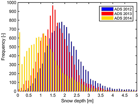
Figure 6. Frequencies of snow depths for all ADS datasets. The blue bars represents the ADS 2012, the red bars the ADS 2013 and the yellow bars the ADS 2014 dataset. Bin sizes of the histogram is 10 cm. X-axis is cut at 5 m to increase readability.

For the snow depth driven simulations for winter 2013/14, the effect of scaling is also clearly visible in the change of the absolute errors. We assume that not only the ADS data is crucial for good scaling results, but that also the total precipitation mass is important. If too much precipitation is allocated, the scaling will be less effective due to excessive supply of precipitation which leads to a smoothing of the snow cover. The smoothing stems from the fact that the proportional settling of deeper snow is larger than for thinner snow. If the correct or too little precipitation is allocated the scaling has a stronger effect on the correct redistribution. This can be seen when comparing the two simulations for winter 2013/14.

For all simulations using scaling, a negative drift of the mean error is evident. This is despite the fact that the scaling mechanism conserves the total precipitation mass allocated by the basic, non-scaling method (cf. Equation 1). The shift comes from the settling and melting information in the ADS datasets. The dataset represents a snow distribution toward the end of the winter but is applied to scale precipitation throughout the whole winter. The ADS data already accounts for settled snow depths and partial melting. If it is used for scaling precipitation throughout the whole winter and the model itself accounts for settling and melting on the snow cover too, these effects are overrepresented and lead to an overall reduction of snow volume. Also the local redistribution of precipitation due to scaling leads to different settling effects compared to the base method, leading to a decrease in overall snow depth. The average loss in snow depths is about 10 cm, independent of the precipitation input method.

For all the results presented here, the variation in the simulation setup is only in precipitation input and its interpolation and scaling. All other inputs are kept identical for any simulation. This allows us to best quantify the influence of variations in precipitation input and scaling. On the other hand, we did not quantify the influence and errors in simulation results due to other input quantities and their interpolation. An extended sensitivity analysis on various input quantities using Alpine3D in the Davos area has been conducted by Schölgl et al. (2016). The average vertical accuracy of the ADS data is estimated to ±30 cm (Bühler et al., 2015). For the simulations presented here, we had to assume the ADS data as being accurate to be able to scale precipitation and assess scaling performance. As the scaling methods presented here absolutely require ADS information, the quality of the simulation results highly depend on the available ADS data quality.

3.5. Inter-Annual scaling

If no ADS data is available to scale a specific winter, another dataset can be used. To assess the model performance for such a setting, the winters 2011/12, 2012/13, and 2013/14 have been simulated using [PAT] and were scaled with a different ADS dataset. The influence of a scaling with an ADS dataset from a different winter can be seen in Figure 7. The results from a non-scaling [PSUM] method are also shown for comparison.

FIGURE 7

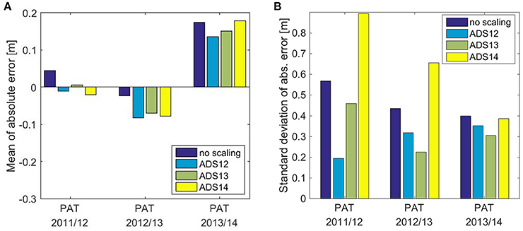
Figure 7. (A) Means and (B) standard deviations of absolute errors of non-scaling simulations (violet) with inter-annual scaling simulations for the winters 2011/12–2013/14. Each scaling simulation was scaled using ADS 2012 (blue), 2013 (green), and 2014 (yellow) dataset for any year simulated.

Figure 7B shows the standard deviation of the absolute error in snow depth for the different simulations. The standard deviation is lowest for any simulation when it was scaled with the ADS dataset from the same year, except for winter 2013/14. Additionally, when being scaled with a different dataset, the standard deviation is lower compared to a non-scaling method, except when using the ADS 2014 dataset to scale the winters 2011/12 and 2012/13.

Comparing the standard deviation for the winters 2011/12 and 2012/13 and the associated ADS datasets only, it can be stated that the scaling method leads to better results than the non-scaling method. This is due to the fact that the ADS snow distribution patterns in the winter 2011/12 and 2012/13 were similar and scaling with either dataset is possible (cf. Figure 6). Using the ADS 2014 dataset to scale other winters leads to worse results than using a non-scaling method. In March and April 2014 the air temperature reached maximum values of over 7°C at 2500 m.a.s.l. for several weeks, leading to intense melting of the snow cover below 2500 m.a.s.l. This information is conserved in the ADS 2014 dataset which was acquired after this period. Therefore, scaling of other winters with this dataset leads to large errors in snow depth distribution with highest errors below 2500 m.a.s.l. in south facing slopes (not shown). Looking at Figure 6, it can be seen that in the ADS 2014 dataset a lot of grid points were already snow free. This influences the scaling strongly as no precipitation is allocated to these grid points. Therefore, the direct scaling mechanism presented here is not suitable to scale precipitation when grid points are snow free. For such cases, the scaling algorithm should be adapted or ADS data must be acquired earlier in the winter when these grid points are still snow covered.

The tests with inter-annual scaling show that the method has the potential to be used with a generalized ADS dataset to scale multiple winters. As only three ADS datasets were available, it was not possible to identify a generally valid snow distribution for the simulation domain. Nevertheless, results shown here indicate that ADS datasets 2012 and 2013 have the potential to be used as a general dataset to scale precipitation in the Davos area. The 2014 dataset was acquired too late and is not suitable for general snow scaling. Further studies using repeat ADS datasets within one winter are needed to find optimal scaling datasets and to assess the temporal consistency of ADS data within one winter and between winters.

3.6. Aspect-Dependency of Scaling Error

For all scaling simulations a relation between error in snow depth and the aspect of the grid point is evident. In north facing slopes the error in snow depth is generally smaller than in south facing slopes (cf. Figure 8B). Looking at non-scaling simulations such as [PSUM] (cf. Figure 8A), we find, however, only a small effect of aspect. For the iterative scaling approach [ALS2], this relation of error and aspect is also still evident (cf. Figure 9). However, compared to our other scaling simulations the amplitude of the error is smaller. We offer three possible explanations for these observations:

1. Using ADS data acquired toward the end of a winter, effects of settling and melting may be overestimated: The information about snow depth stored in the ADS datasets is based on the snow cover toward the end of the winter. Processes causing settling and melting throughout the winter are therefore represented by ADS data and applied on the distribution of precipitation. When the precipitation is distributed on the simulation domain, the model itself also calculates settling and melting. This leads to the problem that these effects are overestimated in the scaled simulations and lead to a strong underestimation of snow depth in slopes where settling is strong and melt has already occurred e.g., in south facing slopes. This can be confirmed when looking at the snow densities in the simulation domain. An analysis of settling and melting occurrence can be found in the Supplementary Material. It can be stated that the error is more dependent on the aspect than on the snow depth. We could show that high densities are more strongly related to thin snow covers in south facing slopes than to thick snow covers in north facing slopes. It is therefore assumed that the effect of radiation influences the snow density more than the gravitation effects due to a thick snow cover. It is therefore concluded that the aspect related errors are mainly caused by the snow settling due to radiation and temperature. Barely any melting had occurred until the date of ADS 2012 data acquisition (analysis of SNOWPACK profiles; not shown). Therefore, we assume that melting effects are negligible compared to settling in this year.

2. The settling of the snow cover is non-linear. Therefore, scaling precipitation does not lead to the same scaling effect in the snow cover. When more precipitation is distributed on a grid point, more snow mass is generated there. The more mass, the more the snow cover is compacted by its own weight. This leads to a disproportional settling of the snow cover.

3. The radiation module used in Alpine3D may calculate too much radiation in south facing slopes: All simulations are run using the simple radiation module in Alpine3D, in which a clearness index is used to split the radiation into direct and diffuse radiation, which is known to sometimes produce unrealistic distributions (Lanini, 2010). If the splitting is overestimating the direct radiation, too much energy is distributed on a grid point, leading to disproportional settling.

FIGURE 8

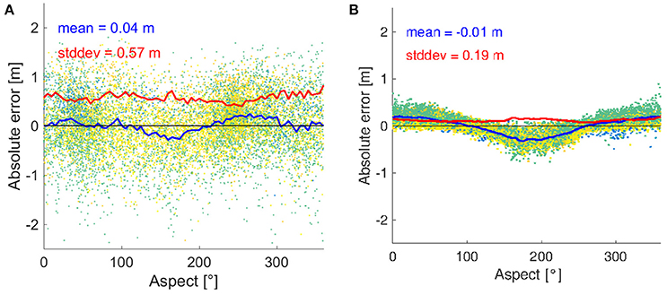
Figure 8. Scatter plot of absolute error of (A) [PSUM] and (B) [PAT] simulations for the winter 2011/12 against aspect. The blue (red) line shows the moving average (standard deviation) for different aspects. The colors indicate land use classification of the grid points (green: rock, yellow: alpine meadow, blue: bush).

FIGURE 9

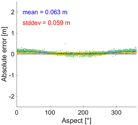
Figure 9. Scatter plot of absolute error of [ALS2] simulation for the winter 2011/12 against aspect. The blue (red) line shows the moving average (standard deviation) for different aspects. The colors indicate land use classification of the grid points (green: rock, yellow: alpine meadow, blue: bush).

To estimate how much of the aspect related error is caused by the three effects described above, a comparison of [PAT] and [HAT] simulations with [ALS2] is suitable. As the iterative [ALS2] scaling is based on the correction of gridded precipitation data for each time step, it is independent of the settling information stored in the ADS datasets (1). Since this comparison shows that iterative scaling has a much smaller remaining error, it can be concluded that effect (1) dominates the aspect-dependent systematic error but that the other effects (2,3) are not negligible.

The error due to the scaling with ADS acquired late in the winter is larger than with an earlier acquisition. An option could be that ADS data is acquired earlier in the winter when less settling (and melting) has occurred. The error due to the radiation partitioning could be reduced by making the partitioning methods more robust. Even though the scaling leads to an aspect-dependent error as discussed, the mean error in distributed snow depths is reduced for most of the scaling methods and simulated winter.

4. Conclusions and Outlook

In this study, a simple precipitation scaling approach was developed and tested with the aim to improve the representation of the spatial distribution of snow in distributed numerical models, while maintaining low computational costs. This method has the potential to significantly improve spatial snow representation in distributed snow modeling without the need for spatially explicit modeling of wind transport (Lehning et al., 2008; Vionnet et al., 2014), which either suffers from high computational demand, limited accuracy or both.

The performance of traditional simulation setups without scaling were tested and it was found that methods such as the [PSUM] or [HS] are able to generally represent the total snow mass in the simulation domain with good accuracy. However, these methods were found to not represent the total variability of the snow cover and often underestimate large snow depths at high elevations in particular whereas small snow depths are generally overestimated by the methods. Our proposed scaling approach reduced the standard deviation of the absolute error in spatial snow distribution significantly (up to a factor of 3.4) to less than 0.23 m. By choosing an appropriate base method to allocate the precipitation, the mean error of the snow cover could also be reduced to a few centimeters for the simulation domain. For these promising results, only one simulation run is required and one remote sensing dataset is sufficient for scaling. This shows that with the simple scaling method presented here, the overall performance in snow distribution modeling with Alpine3D or other snow models can be significantly improved. An iterative scaling approach [ALS2] is able to further compensate for errors generated in a first simulation run and the mean snow depth as well as the spatial variability are represented with very high accuracy. Drawbacks of iterative scaling are a high computational demand and the necessity to write, store and re-read large amounts of data.

Tests with inter-annual scaling showed that scaling approaches based on ADS measurements from a different year lead to good results as long as the relative snow distribution is represented in the remote sensing data used for scaling. It is therefore possible to use one remote sensing dataset to scale various winters (Lehning et al., 2011). scaling becomes less accurate only when the remote sensing data set has a large portion of little snow and snow free grid points. Then the risk of assigning too little or no precipitation to a grid point increases dramatically.

The performance of the scaling method depends on the quality of the remote sensing data. As this data fully determines how the precipitation is distributed and where a snow cover develops, its quality is critical in obtaining accurate snow depth distributions in the simulation. Errors in ADS data are difficult to identify, if the simulation output is compared to the remote sensing data. Therefore, it is important to use independent observations to verify the simulations results. In this respect, our inter-annual experiments can be seen as a successful cross-validation. To compare the simulation outputs with independent data, observations from AWSs are in principle a good choice. However, the station must be representative for its vicinity to allow a direct comparison, which is generally difficult for this type of terrain (Grünewald and Lehning, 2015). A very high grid resolution facilitates such a comparison. In this work it was not possible to find a suitable AWS to compare with the simulation results at the grid resolution of 100 m. Due to the extensive size of the simulation domain it was not feasible to further increase the simulation grid resolution within the context of this study.

In this study, it could be shown that the scaling method can substantially increase simulation performance regarding snow distribution although this method also brings along undesired effects leading to errors. The major drawback of the method is that it is sensitive to snow settling, melting and the date of ADS data acquisition. If remote sensing data are acquired from a snow cover where settling or melting has occurred, these effects influence the model and too little precipitation is allocated. This leads to an underestimation of the snow depth in certain areas. This not only decreases the performance of the spatial snow distribution simulation but can also have a major influence on the total snow volume in the simulation domain. To date, it was not possible to solve this issue, but it is assumed that with earlier snow depth acquisitions, the errors can further be reduced. Solving this issue is an important but also a challenging task in order to make more operational use of our scaling method in numerical snow modeling.

As an outlook on further work, a next step is to acquire more snow depth maps following individual storms and earlier in the winter. As briefly discussed above and shown in the Supplementary Material, a reasonable validation of time-resolved snow depth development at local weather stations is currently not possible. Based on temporal snow depth maps, the seasonal development can be studied in more detail and some of the errors discussed in our contribution can certainly be reduced. Along these lines, it is also interesting to decompose the weighting factor into a more regional simple trend, which takes larger-scale moisture gradients as well as the classical elevation into account. This base field can be applied to liquid and solid precipitation. The finer scale patterns, which can be seen as residuals from the larger-scale field, are then only be applied to snowfall. Finally, it should be studied, in how far spatial estimation of meteorological input other than precipitation amount can be improved to allow an optimized rain—snow distinction, which has a critical influence on our results.

Author Contributions

All authors contributed to this work. This main paper was written by CV and is based on his master thesis. ML designed the study and supervised the working process. NW and MB also supervised the working process and gave assistance using Alpine3D, analysing results and implementing the scaling algorithm. All authors contributed written sections to this paper.

Funding

The paper is based on a master thesis by the first author and institutional funding from SLF Davos as well as EPFL is acknowledged. Furthermore, data and collaborators have partially been funded by the Swiss National Science Foundation (SNF) grants 200021_150146 and 200021E-160667.

Conflict of Interest Statement

The authors declare that the research was conducted in the absence of any commercial or financial relationships that could be construed as a potential conflict of interest.

Acknowledgments

Leica Geosystems (Hexagon) supported us by flying the ADS camera free of charge. We thank Yves Bühler and Mauro Marty for the processing of the ADS data, Charles Fierz and Peter Molnar for the scientific inputs during the realization of the study and Marcia Phillips for proofreading the manuscript. We thank the two Referees and the Editor for their interest in our work and for the helpful comments that helped to improve the manuscript quality. Various institutions contributed with input data for model simulations such as MeteoSwiss, FOEN (Federal Office for the Environment) and the Canton of Grisons. The Alpine3D, MeteoIO and SNOWPACK source code is available under the (L)GPL version 3 at http://models.slf.ch.

Supplementary Material

The Supplementary Material for this article can be found online at: https://www.frontiersin.org/article/10.3389/feart.2016.00108/full#supplementary-material

References

Anslow, F. S., Hostetler, S., Bidlake, W. R., and Clark, P. U. (2008). Distributed energy balance modeling of South Cascade Glacier, Washington and assessment of model uncertainty. J. Geophys. Res. 113:F02019. doi: 10.1029/2007JF000850

CrossRef Full Text | Google Scholar

Bartelt, P., and Lehning, M. (2002). A physical SNOWPACK model for the Swiss avalanche warning: part I: numerical model. Cold Regions Sci. Technol. 35, 123–145. doi: 10.1016/S0165-232X(02)00074-5

CrossRef Full Text | Google Scholar

Bavay, M., and Egger, T. (2014). MeteoIO 2.4.2: a preprocessing library for meteorological data. Geosci. Model Dev. 7, 3135–3151. doi: 10.5194/gmd-7-3135-2014

CrossRef Full Text | Google Scholar

Bavay, M., Lehning, M., Jonas, T., and Löwe, H. (2009). Simulations of future snow cover and discharge in Alpine headwater catchments. Hydrol. Process. 23, 95–108. doi: 10.1002/hyp.7195

CrossRef Full Text | Google Scholar

Bellaire, S., Jamieson, J. B., and Fierz, C. (2011). Forcing the snow-cover model SNOWPACK with forecasted weather data. Cryosphere 5, 1115–1125. doi: 10.5194/tc-5-1115-2011

CrossRef Full Text | Google Scholar

Bühler, Y., Marty, M., Egli, L., Veitinger, J., Jonas, T., Thee, P., et al. (2015). Snow depth mapping in high-alpine catchments using digital photogrammetry. Cryosphere 9, 229–243. doi: 10.5194/tc-9-229-2015

CrossRef Full Text | Google Scholar

Bühler, Y., Marty, M., and Ginzler, C. (2012). High resolution DEM generation in high-alpine terrain using airborne remote sensing techniques. Trans. GIS 16, 635–647. doi: 10.1111/j.1467-9671.2012.01331.x

CrossRef Full Text | Google Scholar

Bühler, Y., Marty, M., and Ginzler, C. (2013). Grossflächige hochaufgelöste Schneehöhenkarten aus digitalen Stereoluftbildern. Geomatik Schweiz Geoinformation und Landmanagement 111, 508–510.

PubMed Abstract

Comola, F., Schaefli, B., Ronco, P. D., Botter, G., Bavay, M., Rinaldo, A., et al. (2015). Scale-dependent effects of solar radiation patterns on the snow-dominated hydrologic response. Geophys. Res. Lett. 42:2015GL064075. doi: 10.1002/2015GL064075

CrossRef Full Text | Google Scholar

Deems, J. S., Painter, T. H., and Finnegan, D. C. (2013). Lidar measurement of snow depth: a review. J. Glaciol. 59, 467–479. doi: 10.3189/2013JoG12J154

CrossRef Full Text | Google Scholar

Endrizzi, S., Gruber, S., Dall'Amico, M., and Rigon, R. (2014). GEOtop 2.0: simulating the combined energy and water balance at and below the land surface accounting for soil freezing, snow cover and terrain effects. Geosci. Model Dev. 7, 2831–2857. doi: 10.5194/gmd-7-2831-2014

CrossRef Full Text | Google Scholar

Gallice, A., Bavay, M., Brauchli, T., Comola, F., Lehning, M., and Huwald, H. (2016). StreamFlow 1.0: an extension to the spatially distributed snow model Alpine3D for hydrological modeling and deterministic stream temperature prediction. Geosci. Model Dev. Discuss. 167, 1–51. doi: 10.5194/gmd-2016-167

CrossRef Full Text | Google Scholar

Gauer, P. (2001). Numerical modeling of blowing and drifting snow in Alpine terrain. J. Glaciol. 47, 97–110. doi: 10.3189/172756501781832476

CrossRef Full Text | Google Scholar

Goodison, B., Louie, P., and Yang, D. (1998). WMO Solid Precipitation Measurement Intercomparison–Final Report. Technical Report 67, WMO/TD 872.

Grünewald, T., and Lehning, M. (2011). Altitudinal dependency of snow amounts in two small alpine catchments: can catchment-wide snow amounts be estimated via single snow or precipitation stations? Ann. Glaciol. 52, 153–158. doi: 10.3189/172756411797252248

PubMed Abstract | CrossRef Full Text | Google Scholar

Grünewald, T., and Lehning, M. (2015). Are flat-field snow depth measurements representative? A comparison of selected index sites with areal snow depth measurements at the small catchment scale. Hydrol. Process. 29, 1717–1728. doi: 10.1002/hyp.10295

CrossRef Full Text | Google Scholar

Grünewald, T., Schirmer, M., Mott, R., and Lehning, M. (2010). Spatial and temporal variability of snow depth and ablation rates in a small mountain catchment. Cryosphere 4, 215–225. doi: 10.5194/tc-4-215-2010

CrossRef Full Text | Google Scholar

Groot Zwaaftink, C. D., Löwe, H., Mott, R., Bavay, M., and Lehning, M. (2011). Drifting snow sublimation: a high-resolution 3-D model with temperature and moisture feedbacks. J. Geophys. Res. 116:D16107. doi: 10.1029/2011JD015754

CrossRef Full Text | Google Scholar

Hanzer, F., Helfricht, K., Marke, T., and Strasser, U. (2016). Multilevel spatiotemporal validation of snow/ice mass balance and runoff modeling in glacierized catchments. Cryosphere 10, 1859–1881. doi: 10.5194/tc-10-1859-2016

CrossRef Full Text | Google Scholar

Heimo, A., Calpini, B., Konzelmann, T., and Suter, S. (2007). SwissMetNet: The New Automatic Meteorological Network of Switzerland. Technical report, MeteoSwiss, Zurich.

Helbig, N. (2009). Application of the Radiosity Approach to the Radiation Balance in Complex Terrain. Dissertation, University of Zürich, Zürich.

Huss, M., Bauder, A., Funk, M., and Hock, R. (2008). Determination of the seasonal mass balance of four Alpine glaciers since 1865. J. Geophys. Res. 113:F01015. doi: 10.1029/2007JF000803

CrossRef Full Text | Google Scholar

Koenig, U., and Abegg, B. (1997). Impacts of climate change on winter tourism in the Swiss alps. J. Sustain. Tour. 5, 46–58. doi: 10.1080/09669589708667275

CrossRef Full Text | Google Scholar

Kresse, W., and Danko, D. M. (2012). Springer Handbook of Geographic Information. Dordrecht: Springer Science & Business Media.

Google Scholar

Lanini, F. (2010). Division of Global Radiation Into Direct Radiation and Diffuse Radiation. Master thesis, University of Bern, Bern.

Google Scholar

Lehning, M., Bartelt, P., Brown, B., and Fierz, C. (2002a). A physical SNOWPACK model for the Swiss avalanche warning: part III: meteorological forcing, thin layer formation and evaluation. Cold Regions Sci. Technol. 35, 169–184. doi: 10.1016/S0165-232X(02)00072-1

CrossRef Full Text | Google Scholar

Lehning, M., Bartelt, P., Brown, B., Fierz, C., and Satyawali, P. (2002b). A physical SNOWPACK model for the Swiss avalanche warning: part II. Snow microstructure. Cold Regions Sci. Technol. 35, 147–167. doi: 10.1016/S0165-232X(02)00073-3

CrossRef Full Text | Google Scholar

Lehning, M., Bartelt, P., Brown, B., Russi, T., Stöckli, U., and Zimmerli, M. (1999). Snowpack model calculations for avalanche warning based upon a new network of weather and snow stations. Cold Regions Sci. Technol. 30, 145–157. doi: 10.1016/S0165-232X(99)00022-1

CrossRef Full Text | Google Scholar

Lehning, M., Grünewald, T., and Schirmer, M. (2011). Mountain snow distribution governed by an altitudinal gradient and terrain roughness. Geophys. Res. Lett. 38:L19504. doi: 10.1029/2011GL048927

CrossRef Full Text | Google Scholar

Lehning, M., Löwe, H., Ryser, M., and Raderschall, N. (2008). Inhomogeneous precipitation distribution and snow transport in steep terrain. Water Resour. Res. 44:W07404. doi: 10.1029/2007WR006545

CrossRef Full Text | Google Scholar

Lehning, M., Völksch, I., Gustafsson, D., Nguyen, T. A., Stähli, M., and Zappa, M. (2006). ALPINE3d: a detailed model of mountain surface processes and its application to snow hydrology. Hydrol. Process. 20, 2111–2128. doi: 10.1002/hyp.6204

CrossRef Full Text | Google Scholar

Liston, G. E., and Sturm, M. (1998). A snow-transport model for complex terrain. J. Glaciol. 44, 498–516.

Google Scholar

Magnusson, J., Gustafsson, D., Hüsler, F., and Jonas, T. (2014). Assimilation of point SWE data into a distributed snow cover model comparing two contrasting methods. Water Resour. Res. 50, 7816–7835. doi: 10.1002/2014WR015302

CrossRef Full Text | Google Scholar

Michlmayr, G., Lehning, M., Koboltschnig, G., Holzmann, H., Zappa, M., Mott, R., et al. (2008). Application of the Alpine 3d model for glacier mass balance and glacier runoff studies at Goldbergkees, Austria. Hydrol. Process. 22, 3941–3949. doi: 10.1002/hyp.7102

CrossRef Full Text | Google Scholar

Mott, R., Schirmer, M., and Lehning, M. (2011). Scaling properties of wind and snow depth distribution in an Alpine catchment. J. Geophys. Res. 116:D06106. doi: 10.1029/2010JD014886

CrossRef Full Text | Google Scholar

Prokop, A., Schirmer, M., Rub, M., Lehning, M., and Stocker, M. (2008). A comparison of measurement methods: terrestrial laser scanning, tachymetry and snow probing for the determination of the spatial snow-depth distribution on slopes. Ann. Glaciol. 49, 210–216. doi: 10.3189/172756408787814726

CrossRef Full Text | Google Scholar

Revuelto, J., Vionnet, V., López-Moreno, J.-I., Lafaysse, M., and Morin, S. (2016). Combining snowpack modeling and terrestrial laser scanner observations improves the simulation of small scale snow dynamics. J. Hydrol. 533, 291–307. doi: 10.1016/j.jhydrol.2015.12.015

CrossRef Full Text | Google Scholar

Schaefli, B., Hingray, B., and Musy, A. (2007). Climate change and hydropower production in the Swiss Alps: quantification of potential impacts and related modelling uncertainties. Hydrol. Earth Syst. Sci. 11, 1191–1205. doi: 10.5194/hess-11-1191-2007

CrossRef Full Text | Google Scholar

Schirmer, M., Wirz, V., Clifton, A., and Lehning, M. (2011). Persistence in intra-annual snow depth distribution: 1. Measurements and topographic control. Water Resour. Res. 47:W09516. doi: 10.1029/2010WR009426

CrossRef Full Text | Google Scholar

Schölgl, S., Marty, C., Bavay, M., and Lehning, M. (2016). Sensitivity of alpine3d modeled snow cover to modifications in DEM resolution, station coverage and meteorological input quantities. Environ. Model. Softw. 83, 387–396. doi: 10.1016/j.envsoft.2016.02.017

CrossRef Full Text | Google Scholar

Schuler, T., Loe, E., Taurisano, A., Eiken, T., Hagen, J., and Kohler, J. (2007). Calibrating a surface mass-balance model for Austfonna ice cap, Svalbard. Ann. Glaciol. 46, 241–248. doi: 10.3189/172756407782871783

CrossRef Full Text | Google Scholar

Schweizer, J., Bruce Jamieson, J., and Schneebeli, M. (2003). Snow avalanche formation. Rev. Geophys. 41:1016. doi: 10.1029/2002RG000123

CrossRef Full Text | Google Scholar

Trujillo, E., Ramírez, J. A., and Elder, K. J. (2007). Topographic, meteorologic, and canopy controls on the scaling characteristics of the spatial distribution of snow depth fields. Water Resour. Res. 43:W07409. doi: 10.1029/2006WR005317

CrossRef Full Text | Google Scholar

Vionnet, V., Martin, E., Masson, V., Guyomarc'h, G., Naaim-Bouvet, F., Prokop, A., et al. (2014). Simulation of wind-induced snow transport and sublimation in alpine terrain using a fully coupled snowpack/atmosphere model. Cryosphere 8, 395–415. doi: 10.5194/tc-8-395-2014

CrossRef Full Text | Google Scholar

Wever, N. (2015). Liquid Water Flow in Snow and Hydrological Implications. Dissertation, Ecole Polytechnique federal de Lausanne EPFL, Lausanne.

Google Scholar

Wever, N., Fierz, C., Mitterer, C., Hirashima, H., and Lehning, M. (2014). Solving Richards Equation for snow improves snowpack meltwater runoff estimations in detailed multi-layer snowpack model. Cryosphere 8, 257–274. doi: 10.5194/tc-8-257-2014

CrossRef Full Text | Google Scholar

Wever, N., Schmid, L., Heilig, A., Eisen, O., Fierz, C., and Lehning, M. (2015). Verification of the multi-layer SNOWPACK model with different water transport schemes. Cryosphere 9, 2271–2293. doi: 10.5194/tc-9-2271-2015

CrossRef Full Text | Google Scholar

Winstral, A., Elder, K., and Davis, R. E. (2002). Spatial snow modeling of wind-redistributed snow using terrain-based parameters. J. Hydrometeorol. 3, 524–538. doi: 10.1175/1525-7541(2002)003<0524:SSMOWR>2.0.CO;2

CrossRef Full Text | Google Scholar

Winstral, A., Marks, D., and Gurney, R. (2013). Simulating wind-affected snow accumulations at catchment to basin scales. Adv. Water Resour. 55, 64–79. doi: 10.1016/j.advwatres.2012.08.011

CrossRef Full Text | Google Scholar

Wipf, S., Stoeckli, V., and Bebi, P. (2009). Winter climate change in alpine tundra: plant responses to changes in snow depth and snowmelt timing. Climat. Change 94, 105–121. doi: 10.1007/s10584-009-9546-x

CrossRef Full Text | Google Scholar

Zappa, M., Pos, F., Strasser, U., Warmerdam, P., and Gurtz, J. (2003). Seasonal water balance of an alpine catchment as evaluated by different methods for spatially distributed snowmelt modelling. Hydrol. Res. 34, 179–202.

Google Scholar