Spatial Downscaling of Alien Species Presences Using Machine Learning

Introduction

The rate at which species are being translocated by humans beyond their native ranges, through a variety of pathways, has been accelerating (Essl et al., 2015). Alien species pose a grave risk to biodiversity, ecosystem services, and human health, and their presence is an important constituent of the global change that we currently face (Vilà et al., 2011; Simberloff et al., 2013; Katsanevakis et al., 2014), hence there is an urgent need for targeted actions for prevention and mitigation. Despite global efforts to tackle biological invasions, so far there is no sign of saturation in the accumulation of alien species (Hulme et al., 2009; Tittensor et al., 2014; Seebens et al., 2017).

A better understanding of the factors controlling alien species introduction, initial dispersal, establishment success, distribution, abundance, spatio-temporal dynamics, and invasiveness is essential for the efficient prioritization of measures to prevent further introductions and mitigate the impacts of invasive alien species (Byers et al., 2002; Thuiller et al., 2006). Reliable fine scale spatio-temporal information of alien species distribution at large scales is thus crucial (Collingham et al., 2000; Giakoumi et al., 2016). However, the spatial resolution of available data often poses limitations in the analyses. For species distribution data, spatial resolution and spatial extent are typically inversely proportional (Collingham et al., 2000). The European Alien Species Information Network (EASIN; Katsanevakis et al., 2015), which has compiled the largest spatial dataset of alien species distribution in Europe, reports species presence data at a 10 × 10 km² spatial resolution and for some species only at country level. Such coarse resolution is often inadequate for the needs of management and research, as data availability up to a point determines the outputs of the analysis in several ways including complexity, generality, utility, and predictive power (Evans et al., 2014; Evans and Moustakas, 2016). Therefore, either more data need to be collected or computational and statistical methods could be used to increase the utility of readily available data and the reliability of the analyses. To that end, accurate methods for downscaling coarse spatial data can be extremely useful in assessments of environmental and socio-economic impacts of alien species and in management interventions for mitigation.

Based on the fundamental assumption that detectable relationships exist between information across spatial scales, spatial downscaling refers to the process and methodologies of using coarse resolution input to infer finer resolution output. Although, it has extensively been used in other scientific disciplines (Trzaska and Schnarr, 2014), downscaling is not a trivial process. Keil et al. (2013) lists four strictly computational approaches that have been used to predict fine-gridded species presence based on a coarse grid. Assumptions made by direct and iterative approaches (Keil et al., 2013) are often criticized for speculating similar species association with environmental variables across scales (Menke et al., 2009). On the other hand, point sampling and clustering approaches make assumptions regarding habitat suitability within the coarse grid (Keil et al., 2013). In their review, Trzaska and Schnarr (2014) distinguish downscaling methods between the relatively straight-forward but normality-limited linear methods (e.g., delta method, simple and multiple linear regression, canonical-correlation analysis, etc.) and the more versatile but data-intensive and extrapolation-limited non-linear methods (e.g., analog method, cluster analysis, artificial neural networks, self-organizing maps, etc.).

Since essentially spatial downscaling is largely based on the inter-relationship between local and large-scale properties, given the absence of fine scale alien species data, potential environmental explanatory covariates available at the resolution of the alien species, as well as at finer resolutions, could be used to infer alien species presences at finer resolutions. While data on alien species presences may be scarce, environmental data may be readily available. Recent advances in remote sensing, social networks, and digital technology resulted in the availability of large spatially and temporally explicit datasets (Moustakas, 2017). Ecology, epidemiology, and biogeography need to employ novel methods for big data analytics combing statistics and computer science, as the analysis of such datasets requires advanced methods for compiling the data, their visualization, and their analyses (Moustakas, 2017; Moustakas and Evans, 2017). Furthermore, computational methods for data analytics and simulation modeling are facilitated by the existence of increased computer power (Moustakas and Evans, 2015).

Recently, methods that generate numerous classifier functions and aggregate their output, widely referred to as “ensembles methods,” have attracted wide interest. In this context, Random Forest (RF) algorithms are ensembles of decision trees (Breiman et al., 1984), each trained on a randomly sampled subset of the available dataset, thus reducing the chance of overfitting (Breiman, 2001). In the domain of ecology, RFs have been applied for tropical forest carbon mapping using LiDAR (Light Detection and Ranging)-based carbon estimates (Mascaro et al., 2014), downscaling of global livestock census data (Nicolas et al., 2016), occurrence of fish species in relation to environmental variables (Vezza et al., 2015), forest health and vitality in relation to climate and air pollution parameters (Vitale et al., 2014), classification of tree species using an ensemble of remote sensing data (Naidoo et al., 2012), and vegetation spatial distribution assessment under current and future climate scenarios (Prasad et al., 2006). Especially regarding alien species, RFs have been used for mapping of presence using spatial (Peerbhay et al., 2016) or spatiotemporal (Dorigo et al., 2012) analysis of remote sensing data, prediction of presence based on environmental variables (Cutler et al., 2007; Jarošík et al., 2011), and invasion risk assessment based on biogeographical and life-history variables (Chen et al., 2015).

Here we showcase the applicability of spatial downscaling alien species presences using data from vascular plant species coupled with environmental, potential explanatory, covariates comprised of climatic, soil, habitat, and land use indicators at a finer resolution at the Mediterranean island of Crete, Greece. Apart from investigating the potential of using the fine-resolution environmental covariates as predictors for spatial downscaling alien species presences, the developed methodology also assesses the relevant importance of predictors for the downscaling process as well as visualizing and quantifying their actual response on alien species presences. Furthermore, considering an operational framework for assessing presence, the methodology integrates the use of a detection sensitivity threshold.

Case Study

The Island of Crete

Covering an area of 8,700 km², Crete is the largest and most populated island of Greece, and the fifth largest in the Mediterranean. According the Köppen classification, Crete has a Mediterranean—Semiarid climate featuring long and dry summers, and relatively wet and cold winters (Kottek et al., 2006). Crete receives on average about 7.7 billion m³ of rainfall, of which only and 10–15% produces runoff, while 68–76% evapotranspires and 14–17% infiltrates (Koutroulis et al., 2016). The intense tectonic history has formed the island's complex topography that ranges from sea level to 2,450 m, and is abundant in small, ephemeral watersheds (Tsanis et al., 2011). This highly-rugged terrain has been definitive for human development as well as its spatial allocation (Koutroulis et al., 2016). Similarly, this variability has spurred the development of the wide variety of biotopes present on the island (Sfikas, 1987), ranging from coastal to alpine, and the reciprocal plethora of endemic and rare species that constitute one of the 10 biodiversity hotspots in the Mediterranean (Medail and Quezel, 1997) numbering 1,624 native and 47 introduced vascular floral species (Turland et al., 1993). The importance of this biodiversity is highlighted by the fact that over 30% of the island has been included in the Natura 2000 protected area network (Dimitrakopoulos et al., 2004).

Plant Data

Maps of presence-absence of vascular plant species distributions in Crete were digitized from Turland et al. (1993) and its latest supplement (Chilton and Turland, 2004). The island of Crete and its surrounding islets were divided into 162 grid cells, each covering an area of 8.25 × 8.25 km², following the grid cell size of Turland et al. (1993). On each cell, the native, endemic, and alien species richness was calculated. We used (Turland et al., 1993; Chilton and Turland, 2004; and references therein) to define native (nnat = 1,395) and endemic (nend = 174) species, and the vascular plants from D'Agata et al. (2009) that are listed in Chilton and Turland (2004) and Turland et al. (1993) were used to define alien species richness. Only species present in at least two cells were used (nalien = 47). Coarse-grid information was estimated by aggregating this dataset by a factor of two, thus reducing resolution to grid cells of 16.5 × 16.5 km². The spatial distribution of the original as well as the resampled data regarding alien species presences are visualized in Figure 1. All input variables and their ranges (min – max values within each cell) are listed in Table 1.

FIGURE 1

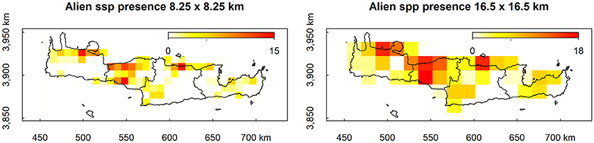
Figure 1. Original (Left) and resampled (Right) spatial distribution of alien species presence in Crete.

TABLE 1

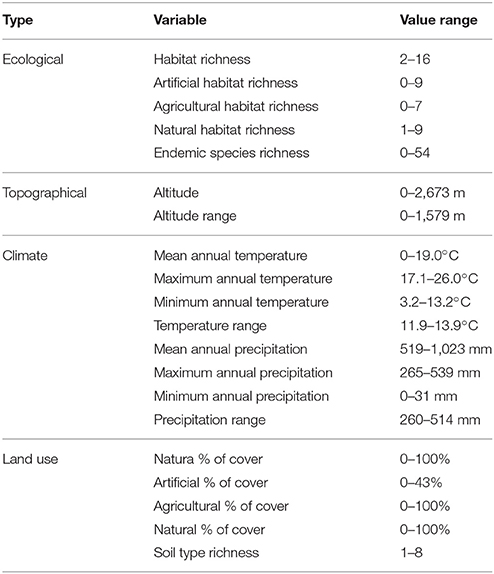
Table 1. Environmental variables used as input for the estimation of alien species presence.

Habitat Data

Habitat classification relied on the most detailed resolution available of the CORINE Landcover (level 3, spatial resolution 100 m; EEA-ETC/TE., 2002), to calculate the richness and percentage of every land cover class within every grid cell, using Patch Analyst 5.1 within ArcGIS. In order to avoid potential temporal deviance between habitat classifications and species presences in cells, the last updated available supplement for the flora of Crete published in 2008 (Chilton and Turland, 2004) and the closest available time snapshot of the CORINE landcover for Crete in 2010 were used. The classification process resulted in 29 habitat types, of which 9 agricultural, 7 artificial, and 13 natural. We recorded habitat richness per cell as the number of different land cover types present on each cell (total, artificial, agricultural, and natural habitat richness) as well as percentage of cover (total, artificial, agricultural, and natural % of cell cover).

Climatic, Soil, and Altitude Data

Climatic variables were derived from WorldClim (Hijmans et al., 2005) for Crete and surrounding islets. The original resolution of the climatic data was 1 × 1 km². In order to re-scale them to 8.25 km and match them with the grid of the plant data, the mean values of the 1 km data within the 8.25 km cells were calculated and used. The climatic variables used were annual mean temperature (Tempmean), annual mean temperature of warmest quarter (Tempwarm), annual mean temperature of coldest quarter (Tempcold), all in °C, annual mean precipitation (Precipmean), precipitation of wettest quarter (Precipwet), and precipitation of driest quarter (Precipdry), all in mm year⁻¹. Soil data were derived from SoilGrid (Hengl et al., 2014) and rescaled from 1 to 8.25 km as the climatic data. The soil variable used was soil richness in the cell (Soildiv) derived as the number of different soil types occurring within each cell. The indices of elevation recorded were the mean of all elevation values within the cell (Alt) and the range of elevation within the cell (Alt range) both in meters.

Methodology

Random Forests

Random Forests (RFs; Breiman, 2001) take advantage of boosting (Schapire et al., 1998) and bagging (bootstrap aggregating; Breiman, 1996a) of the Classification And Regression Tree (CART; Breiman et al., 1984) model, and adapt a more random but nevertheless more efficient node splitting strategy than standard CARTs (Liaw and Wiener, 2002). In RFs, each individual tree is developed after the following steps: (1) Given a set of training data N, n random samples with repetition (bootstrap) are taken as training set; (2) For each node of the tree, M input variables are determined, and m ≪ M, variables are selected for each node. The most important variable randomly chosen is used as a node. The value of m remains constant; (3) Each tree is developed to its maximum expansion.

RFs have been employed in a wide variety of classification and prediction problems (Scornet et al., 2015; Cano et al., 2017) as they are among the most effective computationally-intensive algorithms to extract information from unstable estimates (Scornet et al., 2015). They are especially well suited for large, high-dimensional datasets, where problem complexity and scale render direct discovery of a good model in a single step impossible (Büchlmann and Yu, 2002; Kleiner et al., 2014; Wager et al., 2014). The fact that RFs require tuning of only two parameters (the tree population in each forest and the number of input variables m randomly selected at each node) for which they are usually not very sensitive (Liaw and Wiener, 2002), and their accuracy and competence when faced with scarce, multivariate datasets of intricate structure (Scornet et al., 2015), have greatly contributed to their popularity.

Similar to other data-driven approaches, RFs may not perform equally well when the task at hand is extrapolatory beyond the range of the recovered predictor-predictand relationship or involves scenario analysis (Daliakopoulos and Tsanis, 2016). Furthermore, Strobl and Boulesteix (2007) showed that variable importance measures of the original RF algorithm may be biased due to differences among predictor structure and scale, adding to the interpretability challenges of data-driven methods. Nevertheless, an extensive data-driven model inter-comparison by Fernández-Delgado et al. (2014) showed that they may be the first weapon of choice for real-world problems.

Evaluation Criteria

Typically, CARTs error is estimated following the out-of-bag (OOB) error R(D) of a selection of the input observations based on bagging, otherwise an OOB sample D (James et al., 2013). In RFs, for each tree t, prediction error of D is estimated before and after randomly permuting the values of the j-th variable, thus giving $R\left(D_n^t\right)$ and $R\left(D_n^{tj}\right)$, respectively. Typically, imbalanced datasets favor correct classification of the majority class, nevertheless, RFs can account for this bias by adjusting the voting cut-off from the default 1/c, where c is the number of classes. This provides additional flexibility to the RF algorithm (Ma et al., 2006) and allows for favoring sensitivity or specificity to different classes. A variable can be considered a strong predictor when permuting it increases the prediction error (Gregorutti et al., 2017), therefore it's importance I_V can be defined as:

$\begin{array}{ll}{I}_V\left(X_j, t\right)=R\left(D_n^{tj}\right)-R\left(D_n^t\right)& (1)\end{array}$

The Mean Decrease in Accuracy (MDA) is estimated by averaging this difference over all trees, and normalizing it by the standard deviation of the differences. The more the accuracy of the RF decreases due to the exclusion (or permutation) of a single predictor, the more important that predictor is considered, and therefore variables with a large MDA are more important for data classification.

Gini is one of the most encountered impurity functions, providing a measure of the “goodness-of-split” for CARTs by favoring splits that allocate a single pure node for the largest class and the rest for the remaining classes (Breiman, 1996b). The Gini index for a node t can be calculated as:

$\begin{array}{ll}{I}_G\left(t\right)={\displaystyle \sum _{i\ne j}^{c}p\left(i|t\right)p\left(j|t\right)=1-}{\displaystyle \sum _j^{c}p{\left(j|t\right)}^2}& (2)\end{array}$

where c is the number of classes and p(i|t), p(j|t) are the estimated probabilities of classes i, j at node t (Cano et al., 2017). In this context, Mean Decrease Gini (MDG) aggregates the Gini gain over all splits and trees to assess the classifying capacity of a variable (Friedman et al., 2009) and is thus a metric of the homogeneity of nodes and leaves in the RF (Bluemke and Stepień, 2016).

MDA and MDG can rank each independent variable for its effectiveness as a predictor of alien species richness, but don't show or quantify the actual positive, negative, humped, etc. relationship between them. Nevertheless, this is an elementary process under conditions of multiple acting variables (Häring et al., 2012), such as cumulative human impacts. For this reason, partial dependence plots (Friedman, 2001; Friedman et al., 2009) can be used to depict the relationship of alien species presence probability on each predictor after averaging out the effects of all classification predictors (Cutler et al., 2007).

Finally, the Receiver Operating Characteristics (ROC) analysis has been an indispensable tool for signal detection and diagnostic systems. As documented by Pontius and Si (2014), ROC has been employed in a wide range of applications requiring a threshold-independent measure to compare predicted against observed values. ROC plots have been previously considered in plant ecology, both at a theoretical (Guisan and Zimmermann, 2000) and applied (Manel et al., 2002; Wang et al., 2014) level as effective indicators of model performance independent of the threshold probability. Typically, ROC curves depict true positive rate (TPR), otherwise sensitivity, recall or hit rate, against true negative rate (TNR), otherwise called specificity. In terms of model estimates, TPR and TNR are defined as:

$\begin{array}{ll}TPR{=}^{TP}{╱}_P=\frac{TP}{TP+FN}& (3)\end{array}$

$\begin{array}{ll}TNR{=}^{TN}{╱}_N=\frac{TN}{TN+FP}& (4)\end{array}$

where T, F, P, and N stand for true, false, positive and negative, respectively. The complementary values of TPR and TNR are false negative rate (FNR), otherwise miss rate, and false positive rate (FPR), otherwise fall-out or false alarm. Based on these values, the Matthew's correlation coefficient (MCC; Matthews, 1975), a reduction of the Pearson correlation coefficient for binary variables (Baldi and Brunak, 2001), is a popular evaluation criterion of machine learning performance (Bhasin and Raghava, 2004; Chen et al., 2004; Bao and Cui, 2005):

$\begin{array}{ll}MCC=\frac{TP\times TN-FP\times FN}{\sqrt{\left(TN+FN\right)\left(TN+FP\right)\left(TP+FN\right)\left(TP+FP\right)}}& (5)\end{array}$

MCC has an advantage in imbalanced datasets where the disparity in the number of presence and absence samples is significant.

Random Forest Application

Experiments were developed using the latest (v4.6–12) implementation of Breiman and Cutler's original Fortran code by Liaw and Wiener (2002) in R. While RFs can be trained very efficiently and avoid overfitting (Breiman, 2001), predictions and variable significance ranking are seldom the identical after each random training, especially for small datasets. To account for this uncertainty, a bootstrapping approach of training multiple RFs is adopted. For each training iteration k, RF_k is presented with 70% of the dataset, sampled with replacement, and the remaining is reserved for testing. Presenting only part of the dataset to the RFs also simulates operational use where only part of the study area is sampled at fine grid and the rest is sampled at coarse-grid resolution. Furthermore, as subsets of alien species presence and absence were imbalanced, training was executed using a variable training cutoff, ranging from 0.1 to 0.9. The full code in R used for the analysis is provided in Supplementary Material.

Results

Importance and Gini

Mean decrease in accuracy (MDA) results as estimated from bootstrap randomizations indicate that, apart from the coarse resolution alien species presence, the percentage of natural cover within each cell was the most important predictor of alien species presence, followed by the endemic species richness, altitude, minimum temperature, and altitude range within each cell (Figure 2, left). From the ones explored here, the least predictive in MDA were artificial habitat richness, temperature range, habitat richness, the percentage of the surface area of each cell within the Natura 2,000 protected area network, and the soil type richness (Figure 2, left). In the latter cases, some bootstrap samples have yielded negative results suggesting that permuting these variables from the predictor vector increases accuracy. Results in Mean Decrease Gini (MDG) are in general agreement with those of MDA, also evaluating natural cover, endemic species richness, and altitude as the most efficient splitting variables (Figure 2, right). Agricultural cover replaces minimum temperature for the MDG rating but both variables score highly for both criteria. The least efficient node splits according to MDG were performed by artificial habitat richness, natural habitat richness, agricultural habitat richness, soil type richness, and temperature range (Figure 2, right). Emphatically, artificial habitat richness is the worst predictor for both metrics, essentially boosting the noise in the dataset.

FIGURE 2

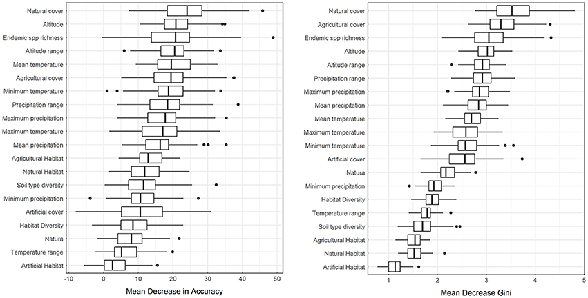
Figure 2. Distribution of Mean Decrease in Accuracy (MDA) and Mean Decrease Gini (MDG) estimated from the bootstrap runs.

Partial Dependence Plots

Results from partial dependence plots among the most predictive variables according to the MDA and MDG criteria indicate that the percentage of natural cover has an overall positive relationship with alien species richness, while the percentage of agricultural cover has an overall negative relationship with alien species richness (Figure 3). Altitude, and altitude range has an overall positive relationship between alien species richness, mean temperature has a negative relationship for larger temperature values while mean annual precipitation and precipitation range has a humped relationship with alien species richness (Figure 3). Therefore, for the case at hand, in the event of a survey priority may be given to low-temperature, elevated natural areas with high topographic variability, far from agricultural use and precipitation extremes. The percentage of each cell within the Natura 2,000 protected area network has a positive relationship with alien species richness (Figure 3), albeit this variable was not within the most predictive of alien species richness based on MDA or MDG.

FIGURE 3

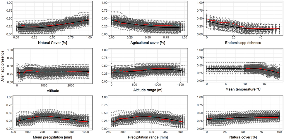
Figure 3. Partial dependence plots for selected independent variables for random forest downscaling of alien species presence. Y-axis is on the logit scale. Here 3rd degree polynomial splines (solid black lines) are fitted over the output the Monte Carlo runs (gray points). Red lines connect points from a single random sample of the bootstrap experiment.

As shown by the results, the bootstrapping method followed herein is helpful for drawing a more robust conclusion, particularly regarding the partial dependence plots. Bootstrapped predictors (solid black lines in Figure 3) are more stable, less prone to overfit and more inclusive than single experiment predictors. This becomes obvious in the Mean Temperature plot of Figure 3, where the red line representing an OOB sample does not cover the entire range of temperature values in the dataset. As low temperatures are not common in the dataset, the OOB estimation of dependence does not always include these values. Using an additional layer of bootstrapping ensures that the full range of values is explored.

Uncertainly and Risk Assessment

True negative detection rates (TNR; not detecting alien species in cells where alien species are not present) declines with an increasing cut-off rate while true positive detection rates (TPR; detecting alien species in cells where alien species are present) increases with an increasing cut-off rate (Figure 4). MCC values indicate a strong positive relationship at cut-offs between 0.2 and 0.5 and are otherwise acceptable correlation. When cut-off increases TNs decrease and TFs increase, therefore more alien species can be detected but by being more exhaustive more false alarms are also generated. When cut-off remains low, less risk is taken with surveying resources but a significant fraction of alien species presences is missed.

FIGURE 4

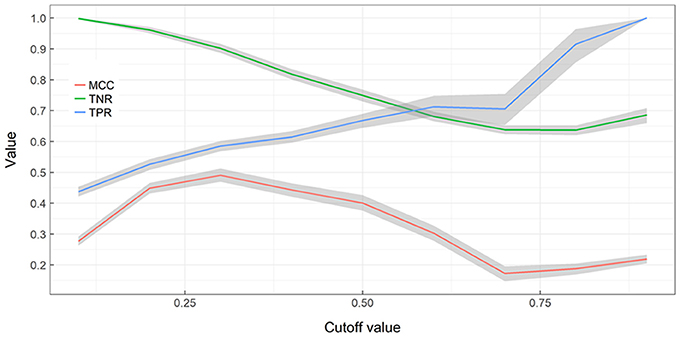
Figure 4. Performance of Random Forest ensemble vs. training cut-off value. A nonparametric bootstrap is used to obtaining confidence limits (gray areas) and bootstrap means for the Matthews correlation coefficient (MCC), True Negative Rate (TNR), True Positive Rate (TPR), without assuming normality.

Discussion

Aichi Target 9 of the Convention on Biological Diversity, states that “by 2020, invasive alien species and pathways are identified and prioritized, priority species are controlled or eradicated and measures are in place to manage pathways to prevent their introduction and establishment.” Prioritization of species, pathways of introduction, and sites for management measures is crucial for the implementation of Aichi Target 9, but the lack of adequate data often compromises the ability of countries to make substantial progress (McGeoch et al., 2016). Large scale, high-resolution data on alien species distributions as well as the associated human and environmental pressures are necessary when performing a spatially explicit quantitative environmental and socio-economic evaluation and prioritizing interventions for their mitigation and management (Hobbs and Humphries, 1995; McGeoch et al., 2016).

It is only evident that substantial part of model output reliability is based on model input validity, thus uncertainty needs to be accounted for (Burgman et al., 2005). Therefore, investment in conservation actions that have been supported by poor field observations has a high probability of yielding poor outcomes (McGeoch et al., 2016), regardless of the subsequent decision process quality. Moreover, ecological processes are often inherently non-linear, and potential explanatory covariates include correlated independent variables, as well as interacting effects. As shown here, RFs can make use of input variables without prior scaling and knowledge of physical or other dependences between predictors and predictands. RFs make no assumptions regarding linearity, handle multiple correlated independent variables well, quantify the importance of each predictor variable, and through partial plots depict the contribution of each independent variable. By assessing the importance of predictors for the desired classification, RFs can effectively permute noisy or otherwise unprofitable data. In addition to enhancing existing model accuracy, this output can have operational value by providing data/survey managers with hints about which data recovery is worth investing in and which not.

Decision makers' requirements for confronting environmental risks and prioritizing mitigation measures at fine grid scale are often much higher than what model limitations and data availability allow. In these cases, a commonly used approach is to employ statistical tools in order to infer impacts at the required scale (Trzaska and Schnarr, 2014). It is crucial to identify and evaluate the premises under which analyses and techniques are used to deduce such output, and to recognize their constraints and inherent uncertainties. In the case of alien species presence downscaling, the approach relies on the assumption that fine-resolution presence is a combination of a coarse-grid presence assessment and environmental conditions, and fine-grid environmental conditions. A common drawback of such approaches is that inherent uncertainties from both initial projections and downscaling procedure are not quantified or adequately conveyed to decision makers and end-users, thus creating an over-confidence to the inferred results and causing validation and updating of downscaled information to be omitted.

Here we have performed spatial downscaling of alien species presences using a relatively idiosyncratic and tricky dataset: the spatial distribution of alien species is clustered, the spatial sample size in terms of the number of cells of the grid of the study area are limited (162 cells in total), and the study area is an island meaning that there are edge effects, unequal land surface areas in coastal cells than in mainland cells, and a very idiosyncratic physical geography, as the island has over 50 mountain summits above 2,000 m (Vogiatzakis et al., 2003). Despite this, the method worked well in the sense that environmental data/covariates of finer scale than the ones of alien species presences can produce finer resolution alien species presences spatial data, and predicted presences or absences were verified and thus the predictive accuracy is explicitly quantified. While additional validation studies in different spatial contexts may highlight other downscaling determining variables, this study outlines an exploratory analysis for variable selection and operational use where underlying environmental information is available at higher resolution. In view of new, spatially and temporally richer data sources (e.g., remote sensing products), results of the present study can be greatly enhanced. Starting from a cost-effective targeted survey design based on the proposed downscaling approach, an improved alien species mapping result can be reached. Beyond the downscaling process itself, a better understanding of alien species distribution and environmental factors that facilitate their presence on the island can be achieved.

Furthermore, the RF architecture allows for tuning toward operationally optimal sensitivity and specificity, thus providing a decision support tool for designing a resource-efficient alien species census. For example, according to one of the most updated alien species dataset in Europe, the distribution of alien plant species appears to be highly clustered with some countries such as the UK, Germany and France appearing to contain the majority of alien species (EASIN dataset; see Figure 5 and references therein). This is unlikely to reflect the actual situation; alien species sampling effort is not evenly distributed among countries and even within countries some areas are better sampled than others. Using the approach proposed here, areas where alien species are not detected but are likely to occur and thus detected once sampled as well as areas where alien species are not detected but are unlikely to occur once sampled can be identified. Additionally, the acceptable risk of false negative and false positive occurrences, also reflecting field detection effort and human labor, can be quantified. In this study, the predicted variable was alien species richness of all alien species, however, given the number of alien species records in the EASIN dataset, the analysis performed here can be adapted at single species level.

FIGURE 5

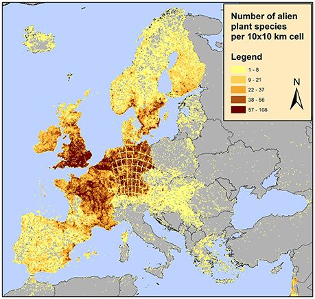
Figure 5. Distribution of alien plants in Europe on a 10 × 10 km² grid according to the available data in the European Alien Species Information Network (EASIN; Katsanevakis et al., 2015). These spatial data, integrated in EASIN, originate from the following sources: (1) the Global Biodiversity Information Facility (GBIF; http://www.gbif.org/); (2) the Global Invasive Species Information Network (GISIN; http://www.gisin.org); (3) the Regional Euro-Asian Biological Invasions Centre (REABIC; http://www.reabic.net/); (4) the European and Mediterranean Plant Protection Organization (EPPO; http://www.eppo.int/); (5) the Norwegian Biodiversity Information Centre (NBIC, http://www.biodiversity.no/) and (6) EASIN-Lit (http://easin.jrc.ec.europa.eu/About/EASIN-Lit; Trombetti et al., 2013).

Conclusions

The science needs for conducting research on biological invasions and the policy needs for management prioritization to prevent further introductions and to mitigate the impacts of invasive alien species, include high-resolution spatiotemporal data of species distributions. We herein demonstrated the applicability of RFs for spatial downscaling, which is an effective, advantageous and useful approach when environmental data are available at better resolution than that of alien species' spatial information. In relation to other downscaling approaches, RFs don't rely on assumptions about environmental parameters and their effect on alien species presence; rather these relationships emerge from the classification process. This way, RFs can provide a better understanding of facilitating and limiting factors of alien species presence, both for research and management purposes. By effectively downscaling coarse-grid alien presence, the RFs can facilitate targeted actions for prevention and mitigation, thus providing an operational exploration tool.

Author Contributions

ID developed the methodology and code, and analyzed the results, SK framed the work within the international context and analyzed results, and AM had the idea, contributed the data, and analyzed the results. All authors contributed equally to the writing process.

Conflict of Interest Statement

The author ID was employed by company TM Solutions.

The other authors declare that the research was conducted in the absence of any commercial or financial relationships that could be construed as a potential conflict of interest.

Supplementary Material

The Supplementary Material for this article can be found online at: https://www.frontiersin.org/article/10.3389/feart.2017.00060/full#supplementary-material

References

Baldi, P., and Brunak, S. (2001). Bioinformatics : The Machine Learning Approach. MIT Press.

Google Scholar

Bao, L., and Cui, Y. (2005). Prediction of the phenotypic effects of non-synonymous single nucleotide polymorphisms using structural and evolutionary information. Bioinformatics 21, 2185–2190. doi: 10.1093/bioinformatics/bti365

PubMed Abstract | CrossRef Full Text | Google Scholar

Bhasin, M., and Raghava, G. P. S. (2004). ESLpred: SVM-based method for subcellular localization of eukaryotic proteins using dipeptide composition and PSI-BLAST. Nucleic Acids Res. 32, W414–W419. doi: 10.1093/nar/gkh350

PubMed Abstract | CrossRef Full Text | Google Scholar

Bluemke, I., and Stepień, A. (2016). Selection of Metrics for the Defect Prediction. Cham: Springer.

Google Scholar

Breiman, L. (1996a). Bagging predictors. Mach. Learn. 24, 123–140. doi: 10.1007/BF00058655

CrossRef Full Text | Google Scholar

Breiman, L. (1996b). Technical note: some properties of splitting criteria. Mach. Learn. 24, 41–47. doi: 10.1007/BF00117831

CrossRef Full Text | Google Scholar

Breiman, L. (2001). Random forests. Mach. Learn. 45, 5–32. doi: 10.1023/A:1010933404324

CrossRef Full Text | Google Scholar

Breiman, L., Friedman, J., Stone, C., and Olshen, R. (1984). Classification and Regression Trees. New York, NY: CRC Press.

Büchlmann, P., and Yu, B. (2002). Analyzing bagging. Ann. Stat. 30, 927–961. doi: 10.1214/aos/1031689014

CrossRef Full Text | Google Scholar

Burgman, M. A., Lindenmayer, D. B., and Elith, J. (2005). Managing landscapes for conservation under uncertainty. Ecology 86, 2007–2017. doi: 10.1890/04-0906

CrossRef Full Text | Google Scholar

Byers, J. E., Reichard, S., Randall, J. M., Parker, I. M., Smith, C. S., Lonsdale, W. M., et al. (2002). Directing research to reduce the impacts of nonindigenous species. Conserv. Biol. 16, 630–640. doi: 10.1046/j.1523-1739.2002.01057.x

CrossRef Full Text | Google Scholar

Cano, G., Garcia-Rodriguez, J., Garcia-Garcia, A., Perez-Sanchez, H., Benediktsson, J. A., Thapa, A., et al. (2017). Automatic selection of molecular descriptors using random forest: application to drug discovery. Expert Syst. Appl. 72, 151–159. doi: 10.1016/j.eswa.2016.12.008

CrossRef Full Text | Google Scholar

Chen, L., Peng, S., and Yang, B. (2015). Predicting alien herb invasion with machine learning models: biogeographical and life-history traits both matter. Biol. Invasions 17, 2187–2198. doi: 10.1007/s10530-015-0870-y

CrossRef Full Text | Google Scholar

Chen, Y. C., Lin, Y. S., Lin, C. J., and Hwang, J. K. (2004). Prediction of the bonding states of cysteines using the support vector machines based on multiple feature vectors and cysteine state sequences. Proteins Struct. Funct. Bioinform. 55, 1036–1042. doi: 10.1002/prot.20079

PubMed Abstract | CrossRef Full Text | Google Scholar

Chilton, L., and Turland, N. (2004). Flora of Crete: Supplement, I. I., Additions 1997-2004. Available onlie at: Publ. internet http://www. marengowalks

Collingham, Y. C., Wadsworth, R. A., Huntley, B., and Hulme, P. E. (2000). Predicting the spatial distribution of non-indigenous riparian weeds: issues of spatial scale and extent. J. Appl. Ecol. 37, 13–27. doi: 10.1046/j.1365-2664.2000.00556.x

CrossRef Full Text | Google Scholar

Cutler, D. R., Edwards, T. C., Beard, K. H., Cutler, A., Hess, K. T., Gibson, J., et al. (2007). Random forests for classification in ecology. Ecology 88, 2783–2792. doi: 10.1890/07-0539.1

PubMed Abstract | CrossRef Full Text | Google Scholar

D'Agata, C., Skoula, M., and Brundu, G. (2009). A preliminary inventory of the alien flora of Crete (Greece). Bocconea 23, 301–315.

Google Scholar

Daliakopoulos, I. N., and Tsanis, I. K. (2016). Comparison of an artificial neural network and a conceptual rainfall–runoff model in the simulation of ephemeral streamflow. Hydrol. Sci. J. 61, 2763–2774. doi: 10.1080/02626667.2016.1154151

CrossRef Full Text | Google Scholar

Dimitrakopoulos, P. G., Memtsas, D., and Troumbis, A. Y. (2004). Questioning the effectiveness of the natura 2000 special areas of conservation strategy: the case of crete. Glob. Ecol. Biogeogr. 13, 199–207. doi: 10.1111/j.1466-822X.2004.00086.x

CrossRef Full Text | Google Scholar

Dorigo, W., Lucieer, A., Podobnikar, T., and Čarni, A. (2012). Mapping invasive Fallopia japonica by combined spectral, spatial, and temporal analysis of digital orthophotos. Int. J. Appl. Earth Obs. Geoinf. 19, 185–195. doi: 10.1016/j.jag.2012.05.004

CrossRef Full Text | Google Scholar

EEA-ETC/TE. (2002). CORINE Land Cover Update. I& CLC2000 Project.

Essl, F., Bacher, S., Blackburn, T. M., Booy, O., Brundu, G., Brunel, S., et al. (2015). Crossing frontiers in tackling pathways of biological invasions. Bioscience 65, 769–782. doi: 10.1093/biosci/biv082

CrossRef Full Text | Google Scholar

Evans, M. R., Benton, T. G., Grimm, V., Lessells, C. M., O'Malley, M. A., Moustakas, A., et al. (2014). Data availability and model complexity, generality, and utility: a reply to Lonergan. Trends Ecol. Evol. 29, 302–303. doi: 10.1016/j.tree.2014.03.004

PubMed Abstract | CrossRef Full Text | Google Scholar

Evans, M. R., and Moustakas, A. (2016). A comparison between data requirements and availability for calibrating predictive ecological models for lowland UK woodlands: learning new tricks from old trees. Ecol. Evol. 6, 4812–4822. doi: 10.1002/ece3.2217

PubMed Abstract | CrossRef Full Text | Google Scholar

Fernández-Delgado, M., Cernadas, E., Barro, S., and Amorim, D. (2014). Do we need hundreds of classifiers to solve real world classification problems? J. Mach. Learn. Res. 15, 3133–3181. Available online at: http://jmlr.org/papers/v15/delgado14a.html

Google Scholar

Friedman, J. (2001). Greedy function approximation: a gradient boosting machine. Ann. Stat. 29, 1189–1232. doi: 10.1214/aos/1013203451

CrossRef Full Text | Google Scholar

Friedman, J., Hastie, T., and Tibshirani, R. (2009). The Elements of Statistical Learning: Data Mining, Inference, and Prediction. New York, NY: Springer-Verlag.

Google Scholar

Giakoumi, S., Guilhaumon, F., Kark, S., Terlizzi, A., Claudet, J., Felline, S., et al. (2016). Space invaders; biological invasions in marine conservation planning. Divers. Distrib. 22, 1220–1231. doi: 10.1111/ddi.12491

CrossRef Full Text | Google Scholar

Gregorutti, B., Michel, B., and Saint-Pierre, P. (2017). Correlation and variable importance in random forests. Stat. Comput. 27, 659–678. doi: 10.1007/s11222-016-9646-1

CrossRef Full Text | Google Scholar

Guisan, A., and Zimmermann, N. E. (2000). Predictive habitat distribution models in ecology. Ecol. Modell. 135, 147–186. doi: 10.1016/S0304-3800(00)00354-9

CrossRef Full Text | Google Scholar

Häring, T., Dietz, E., Osenstetter, S., Koschitzki, T., and Schröder, B. (2012). Spatial disaggregation of complex soil map units: a decision-tree based approach in Bavarian forest soils. Geoderma 185–186, 37–47. doi: 10.1016/j.geoderma.2012.04.001

CrossRef Full Text | Google Scholar

Hengl, T., de Jesus, J. M., MacMillan, R. A., Batjes, N. H., Heuvelink, G. B. M., Ribeiro, E., et al. (2014). SoilGrids1km — global soil information based on automated mapping. PLoS ONE 9:e105992. doi: 10.1371/journal.pone.0105992

PubMed Abstract | CrossRef Full Text | Google Scholar

Hijmans, R. J., Cameron, S. E., Parra, J. L., Jones, P. G., and Jarvis, A. (2005). Very high resolution interpolated climate surfaces for global land areas. Int. J. Climatol. 25, 1965–1978. doi: 10.1002/joc.1276

CrossRef Full Text | Google Scholar

Hobbs, R. J., and Humphries, S. E. (1995). An integrated approach to the ecology and management of plant invasions. Conserv. Biol. 9, 761–770. doi: 10.1046/j.1523-1739.1995.09040761.x

CrossRef Full Text | Google Scholar

Hulme, P. E., Pyšek, P., Nentwig, W., and Vilà, M. (2009). Will threat of biological invasions unite the european union? Science 324, 40–41. doi: 10.1126/science.1171111

PubMed Abstract | CrossRef Full Text | Google Scholar

James, G., Witten, D., Hastie, T., and Tibshirani, R. (2013). An Introduction to Statistical Learning, Springer Texts in Statistics. New York, NY: Springer.

Google Scholar

Jarošík, V., Pyšek, P., Foxcroft, L. C., Richardson, D. M., Rouget, M., and MacFadyen, S. (2011). Predicting incursion of plant invaders into kruger national park, South Africa: the interplay of general drivers and species-specific factors. PLoS ONE 6:e28711. doi: 10.1371/journal.pone.0028711

PubMed Abstract | CrossRef Full Text | Google Scholar

Katsanevakis, S., Deriu, I., D'Amico, F., AL, N., and S, P. S. (2015). European alien species information network (EASIN): supporting European policies and scientific research. Manage. Biol. Invasions 6, 147–157. doi: 10.3391/mbi.2015.6.2.05

CrossRef Full Text | Google Scholar

Katsanevakis, S., Wallentinus, I., Zenetos, A., Leppäkoski, E., Çinar, M. E., Oztürk, B., et al. (2014). Impacts of invasive alien marine species on ecosystem services and biodiversity: a pan-European review. Aquat. Invasions 9, 391–423. doi: 10.3391/ai.2014.9.4.01

CrossRef Full Text | Google Scholar

Keil, P., Belmaker, J., Wilson, A. M., Unitt, P., and Jetz, W. (2013). Downscaling of species distribution models: a hierarchical approach. Methods Ecol. Evol. 4, 82–94. doi: 10.1111/j.2041-210x.2012.00264.x

CrossRef Full Text | Google Scholar

Kleiner, A., Talwalkar, A., Sarkar, P., and Jordan, M. I. (2014). A scalable bootstrap for massive data. J. R. Stat. Soc. Ser. B Stat. Methodol. 76, 795–816. doi: 10.1111/rssb.12050

CrossRef Full Text | Google Scholar

Kottek, M., Grieser, J., Beck, C., Rudolf, B., and Rubel, F. (2006). World map of the Köppen-Geiger climate classification updated. Meteorol. Zeitschrift 15, 259–263. doi: 10.1127/0941-2948/2006/0130

CrossRef Full Text | Google Scholar

Koutroulis, A., Grillakis, M., Daliakopoulos, I., Tsanis, I., and Jacob, D. (2016). Cross sectoral impacts on water availability at +2°C and +3°C for east mediterranean island states: the case of crete. J. Hydrol. 532, 16–28. doi: 10.1016/j.jhydrol.2015.11.015

CrossRef Full Text | Google Scholar

Liaw, A., and Wiener, M. (2002). Classification and regression by randomForest. R News 2, 18–22. Available online at: http://www.bios.unc.edu/~dzeng/BIOS740/randomforest.pdf

Google Scholar

Ma, Y., Guo, L., and Cukic, B. (2006). “A statistical framework for the prediction of fault-proneness,” in Advances in Machine Learning Application, eds D. Zhang and J. J.-P. Tsai (Hershey, PA: Idea Group Pub), 480.

Google Scholar

Manel, S., Williams, H. C., and Ormerod, S. J. (2002). Evaluating presence-absence models in ecology: the need to account for prevalence. J. Appl. Ecol. 38, 921–931. doi: 10.1046/j.1365-2664.2001.00647.x

CrossRef Full Text | Google Scholar

Mascaro, J., Asner, G. P., Knapp, D. E., Kennedy-Bowdoin, T., Martin, R. E., Anderson, C., et al. (2014). A Tale of Two “Forests”: random forest machine learning aids tropical forest carbon mapping. PLoS ONE 9:e85993. doi: 10.1371/journal.pone.0085993

PubMed Abstract | CrossRef Full Text | Google Scholar

Matthews, B. W. (1975). Comparison of the predicted and observed secondary structure of T4 phage lysozyme. Biochim. Biophys. Acta Protein Struct. 405, 442–451. doi: 10.1016/0005-2795(75)90109-9

PubMed Abstract | CrossRef Full Text | Google Scholar

McGeoch, M. A., Genovesi, P., Bellingham, P. J., Costello, M. J., McGrannachan, C., and Sheppard, A. (2016). Prioritizing species, pathways, and sites to achieve conservation targets for biological invasion. Biol. Invasions 18, 299–314. doi: 10.1007/s10530-015-1013-1

CrossRef Full Text | Google Scholar

Medail, F., and Quezel, P. (1997). Hot-spots analysis for conservation of plant biodiversity in the mediterranean basin. Ann. Missouri Bot. Gard. 84, 112–127. doi: 10.2307/2399957

CrossRef Full Text | Google Scholar

Menke, S. B., Holway, D. A., Fisher, R. N., and Jetz, W. (2009). Characterizing and predicting species distributions across environments and scales: argentine ant occurrences in the eye of the beholder. Glob. Ecol. Biogeogr. 18, 50–63. doi: 10.1111/j.1466-8238.2008.00420.x

CrossRef Full Text | Google Scholar

Moustakas, A. (2017). Spatio-temporal data mining in ecological and veterinary epidemiology. Stoch. Environ. Res. Risk Assess. 31, 829–834. doi: 10.1007/s00477-016-1374-8

CrossRef Full Text | Google Scholar

Moustakas, A., and Evans, M. R. (2015). Coupling models of cattle and farms with models of badgers for predicting the dynamics of bovine tuberculosis (TB). Stoch. Environ. Res. Risk Assess. 29, 623–635. doi: 10.1007/s00477-014-1016-y

CrossRef Full Text | Google Scholar

Moustakas, A., and Evans, M. R. (2017). A big-data spatial, temporal and network analysis of bovine tuberculosis between wildlife (badgers) and cattle. Stoch. Environ. Res. Risk Assess. 31, 315–328. doi: 10.1007/s00477-016-1311-x

CrossRef Full Text | Google Scholar

Naidoo, L., Cho, M. A., Mathieu, R., and Asner, G. (2012). Classification of savanna tree species, in the Greater Kruger National Park region, by integrating hyperspectral and LiDAR data in a Random Forest data mining environment. ISPRS J. Photogramm. Remote Sens. 69, 167–179. doi: 10.1016/j.isprsjprs.2012.03.005

CrossRef Full Text | Google Scholar

Nicolas, G., Robinson, T. P., Wint, G. R. W., Conchedda, G., Cinardi, G., and Gilbert, M. (2016). Using random forest to improve the downscaling of global livestock census data. PLoS ONE 11:e0150424. doi: 10.1371/journal.pone.0150424

PubMed Abstract | CrossRef Full Text | Google Scholar

Peerbhay, K., Mutanga, O., Lottering, R., and Ismail, R. (2016). Mapping Solanum mauritianum plant invasions using WorldView-2 imagery and unsupervised random forests. Remote Sens. Environ. 182, 39–48. doi: 10.1016/j.rse.2016.04.025

CrossRef Full Text | Google Scholar

Pontius, R. G. Jr., and Si, K. (2014). The total operating characteristic to measure diagnostic ability for multiple thresholds. Int. J. Geogr. Inf. Sci. 28, 570–583. doi: 10.1080/13658816.2013.862623

CrossRef Full Text | Google Scholar

Prasad, A. M., Iverson, L. R., and Liaw, A. (2006). Newer classification and regression tree techniques: bagging and random forests for ecological prediction. Ecosystems 9, 181–199. doi: 10.1007/s10021-005-0054-1

CrossRef Full Text | Google Scholar

Schapire, R. E., Freund, Y., Bartlett, P., and Lee, W. S. (1998). Boosting the margin: a new explanation for the effectiveness of voting methods. Ann. Stat. 26, 1651–1686. doi: 10.1214/aos/1024691352

CrossRef Full Text | Google Scholar

Scornet, E., Biau, G., and Vert, J.-P. (2015). Consistency of random forests. Ann. Stat. 43, 1716–1741. doi: 10.1214/15-AOS1321

CrossRef Full Text | Google Scholar

Seebens, H., Blackburn, T. M., Dyer, E. E., Genovesi, P., Hulme, P. E., Jeschke, J. M., et al. (2017). No saturation in the accumulation of alien species worldwide. Nat. Commun. 8:14435. doi: 10.1038/ncomms14435

PubMed Abstract | CrossRef Full Text | Google Scholar

Sfikas, G. (1987). Wild Flowers of Crete. Athens: Efstathiadis Group.

Google Scholar

Simberloff, D., Martin, J. L., Genovesi, P., Maris, V., Wardle, D. A., Aronson, J., et al. (2013). Impacts of biological invasions: what's what and the way forward. Trends Ecol. Evol. 28, 58–66. doi: 10.1016/j.tree.2012.07.013

PubMed Abstract | CrossRef Full Text | Google Scholar

Strobl, C., and Boulesteix, A. (2007). Bias in random forest variable importance measures: illustrations, sources and a solution. BMC Bioinformatics 8:25. doi: 10.1186/1471-2105-8-25

PubMed Abstract | CrossRef Full Text | Google Scholar

Thuiller, W., Richardson, D. M., Rouget, M., Procheş, Ş., Wilson, J. R. U., Procheş, S., et al. (2006). Interactions between environment, species traits, and human uses describe patterns of plant invasions. Ecology 87, 1755–1769. doi: 10.1890/0012-9658(2006)87[17552.0.CO;2]

PubMed Abstract | CrossRef Full Text | Google Scholar

Tittensor, D. P., Walpole, M., Hill, S. L. L., Boyce, D. G., Britten, G. L., Burgess, N. D., et al. (2014). A mid-term analysis of progress toward international biodiversity targets. Science 346, 241–244. doi: 10.1126/science.1257484

PubMed Abstract | CrossRef Full Text | Google Scholar

Trombetti, M., Katsanevakis, S., Deriu, I., and Cardoso, A. C. (2013). EASIN-Lit: a geo-database of published alien species records. Manag. Biol. Invasions 4, 261–264. doi: 10.3391/mbi.2013.4.3.08

CrossRef Full Text | Google Scholar

Trzaska, S., and Schnarr, E. (2014). A Review of Downscaling Methods for Climate Change Projections. United States Agency Int. Dev.

Tsanis, I. K., Koutroulis, A. G., Daliakopoulos, I. N., and Jacob, D. (2011). Severe climate-induced water shortage and extremes in Crete. Clim. Change 106, 667–677. doi: 10.1007/s10584-011-0048-2

CrossRef Full Text | Google Scholar

Turland, N., Chilton, L., and Press, J. (1993). Flora of the Cretan Area: Annotated Checklist and Atlas. London: JR Press.

Google Scholar

Vezza, P., Muñoz-Mas, R., Martinez-Capel, F., and Mouton, A. (2015). Random forests to evaluate biotic interactions in fish distribution models. Environ. Model. Softw. 67, 173–183. doi: 10.1016/j.envsoft.2015.01.005

CrossRef Full Text | Google Scholar

Vilà, M., Espinar, J. L., Hejda, M., Hulme, P. E., Jarošík, V., Maron, J. L., et al. (2011). Ecological impacts of invasive alien plants: a meta-analysis of their effects on species, communities and ecosystems. Ecol. Lett. 14, 702–708. doi: 10.1111/j.1461-0248.2011.01628.x

PubMed Abstract | CrossRef Full Text | Google Scholar

Vitale, M., Proietti, C., Cionni, I., Fischer, R., and De Marco, A. (2014). Random forests analysis: a useful tool for defining the relative importance of environmental conditions on crown defoliation. Water Air Soil Pollut. 225:1992. doi: 10.1007/s11270-014-1992-z

CrossRef Full Text | Google Scholar

Vogiatzakis, I. N., Griffiths, G. H., and Mannion, A. M. (2003). Environmental factors and vegetation composition, Lefka Ori massif, Crete, S. Aegean. Glob. Ecol. Biogeogr. 12, 131–146. doi: 10.1046/j.1466-822X.2003.00021.x

CrossRef Full Text | Google Scholar

Wager, S., Hastie, T., and Efron, B. (2014). Confidence intervals for random forests: the jackknife and the infinitesimal jackknife. J. Mach. Learn. Res. 15, 1625–1651. Available online at: http://jmlr.org/papers/v15/wager14a.html

PubMed Abstract | Google Scholar

Wang, X. H., Liu, Y. J., and Guo, L. N. (2014). The invasive species risk assessment and prediction system based on GIS. Appl. Mech. Mater. 675–677, 1052–1057. doi: 10.4028/www.scientific.net/AMM.675-677.1052

CrossRef Full Text | Google Scholar