Parameter Tuning for the NFFT Based Fast Ewald Summation

1. Introduction

In this paper we consider the computation of the Coulomb potentials and forces in charged particle systems subject to 3d-periodic boundary conditions. Unfortunately, the underlying infinite sums, which have to be evaluated, are very slowly and even conditionally convergent.

Nevertheless, there are already quite a lot methods for the efficient evaluation of the Coulomb potentials and forces. Most of them, as for instance [1–5], are based on the so called Ewald summation approach [6], which splits the slowly converging sum into two rapidly converging parts, where the underlying order of summation takes a central role. The one part is a sum in spatial domain and can be evaluated efficiently. The other part is a sum in Fourier space. An efficient evaluation with only ${O}$(N log N) arithmetic operations, where N denotes the number of present particles, is possible by applying the fast Fourier transform (FFT). Thereby, the sticking point is that the particles are not distributed on a regular grid. Thus, the present continuous charge distribution has at first to be approximated by a regular grid based charge density.

Algorithms which are based on such an approximation are commonly known as particle mesh methods [1–4, 7, 8]. Most methods use B-splines in order to perform this grid based approximation step, as for example the well-established particle-particle particle-mesh (P³M) method [1, 4]. Also approximations via a Gaussian have already been considered, see Lindbo and Tornberg [5]. The particle-particle NFFT (P²NFFT) approach, which was suggested in Hedman and Laaksonen [9] and Pippig and Potts [7], is based on the FFT for nonequispaced data (NFFT) and allows the usage of various types of approximating window functions, as for example also (Kaiser-)Bessel functions besides B-splines and Gaussian. In this context we remark that in a variety of applications the results strongly depend on which window function is applied. As an example, in the field of magnetic resonance imaging Kaiser-Bessel functions seem most suitable, see Fourmont [10].

Note that Arnold et al. [11] serves a detailed comparison between different efficient methods for the 3d-periodic Coulomb problem. The results show that the P³M and P²NFFT solvers rank among the best methods in this field. We further remark that the P²NFFT method has already been generalized to mixed periodic as well as open boundary conditions, see Nestler et al. [12] and Nestler et al.[13]. The fast multipole method (FMM) [14–17], which scales like ${O}$(N), can also handle all types of periodic as well as open boundary conditions very efficiently, see Kudin and Scuseria [18]. One advantage of Fourier based methods over hierarchical methods, for instance, is the easy handling of non-cubic box geometries. Furthermore, P²NFFT and P³M are comparable to the FMM in terms of runtime as well as parallel efficiency and in certain cases even outperform the FMM. For more details see Arnold et al. [11].

In the present paper we consider the P²NFFT method and discuss how all involved parameters can be tuned appropriately. How do we have to set the NFFT parameters and which window function do we have to choose in order to reach a certain accuracy, while keeping the computational costs as small as possible? In order to answer this question, we consider the root mean square error (rms) in the forces, which is a common error measure in the field of molecular dynamics simulations, and draw some comparisons between different window functions.

The P²NFFT algorithm, which is part of the publicly available ScaFaCoS library [19], allows the computation of an oversampled FFT. The numerical results presented in this paper, see Section 4, show that an appropriate tuning of the oversampling factor is possible based on the presented error estimates. In order to reach a certain accuracy different combinations of oversampling and the support size of the NFFT window function are possible. The results indicate that we can improve the performance of the method by spending some oversampling combined with using a window function having a smaller support. The usage of the Gaussian or the Bessel window makes the tuning somewhat more complicated, since also the shape parameter of the function has to be tuned. If the shape parameter is chosen appropriately, we can even achieve better results with the Bessel window than by using B-Splines. In our numerical examples we could save approximately fifteen percent of runtime via using the Bessel window with oversampling, compared to using B-splines without oversampling. We remark that the P²NFFT method based on the B-spline window without oversampling is mathematically equivalent to the classical P³M approach, see Pippig [20], for instance.

The outline of the paper is as follows. In Section 2 we give an introduction to the NFFT. In Section 3 we consider the Coulomb problem for 3d-periodic boundary conditions and introduce the corresponding Ewald formulas. We also discuss the estimation of the rms force error which results from the truncation of the Ewald sums. In Section 4 we describe the concept of the P²NFFT method, present how the rms errors caused by the NFFT approximations can be estimated a priori and draw some comparisons between different window functions. In addition, we present an efficient method to tune all involved parameters automatically. An overall tuning, which in addition optimizes the set of parameters with respect to runtime, should depend on the used hard- and software. Thus, we may tune the method with respect to runtime for a small particle system by comparing the runtimes obtained for different parameter combinations in order to apply the found optimal set of parameters also to larger systems. We demonstrate the described parameter tuning with the help of some examples, for which we use the ScaFaCoS library [19]. In Section 5 we finish with some conclusions.

2. The Nonequispaced FFT

In the following we give a short introduction to the NFFT in three dimensions. Thereby, we make use of the following symbols and notations. For some $\text{M}=(M_1,M_2,M_3)\in 2{\mathbb{N}}^3$ we define the index set ${I}$_M by

${{I}}_M:=\{-M_{1/2},\dots ,M_{1/2}-1\}\times \dots \times \{-M_{3/2},\dots ,M_{3/2}-1\}.$

For two vectors $\text{x}=(x_1,x_2,x_3)\in {ℝ}^3$ and $\text{y}=(y_1,y_2,y_3)\in {ℝ}^3$ we define the component wise product by $\text{x}\odot \text{y}:=(x_1{y}_1,x_2{y}_2,x_3{y}_3)\in {ℝ}^3$ as well as the inner product via x · y := x₁y₁ + x₂y₂ + x₃y₃ ∈ ℝ. For a vector x ∈ ℝ³ with non vanishing components we set ${\text{x}}^{-1}:=(x_1^{-1},x_2^{-1},x_3^{-1})\in {ℝ}^3$.

Let the coefficients ${\widehat{f}}_{\text{k}}\in ℂ$ for $k\in {{I}}_{\text{M}},\text{M}\in 2{\mathbb{N}}^3$, and some arbitrary nodes ${\text{x}}_j\in {𝕋}^3$, where 𝕋 := ℝ ∕ ℤ ≃ [−½, ½) and j = 1, …, N, be given. We are now interested in a fast evaluation of the trigonometric polynomial

$\begin{array}{rc}f(x):={\displaystyle \sum _{k\in {{I}}_M}{\widehat{f}}_k}{\text{e}}^{-2\pi \text{i}k·x}& (1)\end{array}$

at the given nodes x_j, j = 1, …, N.

The straightforward and exact algorithm for the evaluation of such sums is called nonequispaced discrete Fourier transform (NDFT) and requires ${O}$(N|${I}$_M|) arithmetical operations. The NFFT algorithm [21–27] can be used in order to approximate the sums very efficiently with only ${O}$(|${I}$_M|log|${I}$_M| + N) arithmetic operations. In the following we will give an overview of the main steps.

In principle, the function f is approximated by a sum of translates of a one-periodic function $\tilde{\phi }$, i.e.,

$\begin{array}{ll}f(x)\approx \tilde{f}(x):={\displaystyle \sum _{l\in {{I}}_{\sigma \odot M}}{g}_l}\tilde{\phi }\left(x-l\odot {(\sigma \odot M)}^{-1}\right),\hfill & (2)\end{array}$

where we denote by σ ∈ ℝ³, σ ≥ 1 (component wise) the oversampling factor. In the following we denote the oversampled grid size shortly by M_o := σ ⊙ M. Increasing the oversampling factor means that the trigonometric polynomial f is approximated based on a higher resolution of the interval [−1/2, 1/2), i.e., we expect smaller aliasing errors. The function $\tilde{\phi }$ in Equation (2) is the periodization of a window function φ, which is constructed via a tensor product scheme, i.e., we set

$\begin{array}{l}\tilde{\phi }(x):={\displaystyle \sum _{r\in {\mathbb{Z}}^3}\phi }(x+r),\text{ where }\phi (y)={\displaystyle \prod _{j=1}^3{\phi }_j}(y_j)\hfill \\ \text{for }y=(y_1,y_2,y_3)\in {ℝ}^3.\hfill & (3)\end{array}$

Thereby, φ_j(·) are univariate functions. A transformation of $\tilde{f}$ into Fourier space gives

$\begin{array}{l}f(x)-\tilde{f}(x)={\displaystyle \sum _{k\in {{I}}_{M_{\text{o}}}}\left({\widehat{f}}_k-{\widehat{g}}_k{c}_k(\tilde{\phi })\right)}{\text{e}}^{-2\pi \text{i}k·x}\hfill \\ -{\displaystyle \sum _{r\in {\mathbb{Z}}^3\setminus \left\{0\right\}}{\displaystyle \sum _{k\in {{I}}_{M_{\text{o}}}}{\widehat{g}}_k}}{c}_{k+r\odot M_{\text{o}}}(\tilde{\phi }){\text{e}}^{-2\pi \text{i}(k+r\odot M_{\text{o}})·x},\hfill & (4)\end{array}$

where we denote by $c_{\text{k}}(\tilde{\phi })$ the analytical Fourier coefficients of $\tilde{\phi }$ and {ĝ_k} are the discrete Fourier coefficients of {g_l}.

The idea is now to choose the coefficients ĝ_k appropriately. Then, the coefficients g_l in Equation (2) can be computed via the inverse FFT and the evaluation of the stated sums gives the approximate function values $\tilde{f}({\text{x}}_j)\approx f({\text{x}}_j)$. This might be computationally demanding unless φ is compactly supported on a comparable small domain or at least sufficiently small outside of it. In the latter case we replace the window function $\tilde{\phi }$ in Equation (2) by a truncated version

$\begin{array}{l}{\phi }_{\text{t}}(x):=\phi (x)·{\displaystyle \prod _{j=1}^3\chi [-\frac{m}{{\sigma }_j{M}_j},\frac{m}{{\sigma }_j{M}_j}]}(x_j)\hfill \\ =\{\begin{array}{ll}\phi (x)\hfill & :x\in \underset{j=1}{\overset{3}{{\displaystyle \otimes }}}[-\frac{m}{{\sigma }_j{M}_j},\frac{m}{{\sigma }_j{M}_j}],\hfill \\ 0\hfill & :\text{else}.\hfill \end{array}\hfill & (5)\end{array}$

Thereby, we refer to m ∈ ℕ as the support parameter. Note that we could use different values for m in the single dimensions, but for simplicity we choose the same for all three dimensions.

Considering Equation (4) shows that it is reasonable to set

${\widehat{g}}_k:=\{\begin{array}{ll}{\widehat{d}}_k{\widehat{f}}_k=\frac{{\widehat{f}}_k}{c_k({\tilde{\phi }}_{\text{t}})}\hfill & :k\in {{I}}_M,\hfill \\ 0\hfill & :\text{else,}\hfill & (6)\end{array}$

for which the error measured in the ${L}$₂-norm is given by

$\begin{array}{ll}{\Vert f-\tilde{f}\Vert }_2^2={\displaystyle \sum _{k\in {{I}}_M}{\left|{\widehat{f}}_k\right|}^2}{\displaystyle \sum _{r\in {\mathbb{Z}}^3\setminus \left\{0\right\}}\frac{c_{k+r\odot M_{\text{o}}}^2({\tilde{\phi }}_{\text{t}})}{c_k^2({\tilde{\phi }}_{\text{t}})}}.& (7)\end{array}$

Optimizing the error with respect to the ${L}$₂-norm shows that

$\begin{array}{ll}{\widehat{d}}_k:=\frac{c_k({\tilde{\phi }}_{\text{t}})}{{\displaystyle \sum _{r\in {\mathbb{Z}}^3}{c}_{k+r\odot M_{\text{o}}}^2}({\tilde{\phi }}_{\text{t}})}& (8)\end{array}$

is the optimal choice for the coefficients ${\widehat{d}}_{\text{k}}$, see Duijndam and Schonewille [28], Jacob [29], and Nestler [30]. We end up with

$\begin{array}{ll}{\Vert f-\tilde{f}\Vert }_2^2={\displaystyle \sum _{k\in {{I}}_M}{\left|{\widehat{f}}_k\right|}^2}\frac{{\displaystyle \sum _{r\in {\mathbb{Z}}^3\setminus \left\{0\right\}}{c}_{k+r\odot M_{\text{o}}}^2}({\tilde{\phi }}_{\text{t}})}{{\displaystyle \sum _{r\in {\mathbb{Z}}^3}{c}_{k+r\odot M_{\text{o}}}^2}({\tilde{\phi }}_{\text{t}})}.& (9)\end{array}$

Especially in the case that the Fourier coefficients ${\widehat{f}}_{\text{k}}$ tend to zero rapidly we expect that the two different approaches to choose the coefficients ${\widehat{d}}_{\text{k}}$ lead to approximately the same results, see the numerical examples in Nestler [30].

We summarize the NFFT algorithm as follows. The approximation of the function values $f({\text{x}}_j)\approx \tilde{f}({\text{x}}_j)$ via Equation (2) corresponds to the computation of a discrete convolution for each x_j. This is the third and last step of the algorithm. Thus, we refer to the first step of the NFFT, see Equation (6), as the deconvolution step as well as to ${\widehat{d}}_{\text{k}}$ as the deconvolution coefficients. The step from Fourier space to spatial domain (ĝ_k ↦ g_l) is realized via the ordinary inverse FFT (second step).

The FFT size can be chosen larger than the given number of Fourier coefficients M, which is called oversampling. Choosing σ greater than 1 in the single dimensions increases the computational cost, while we expect smaller aliasing errors. We remark that the oversampling technique has already been considered in the very first articles on nonuniform FFTs, see Dutt and Rokhlin [21] and Beylkin [22].

The problem of evaluating sums of the form

$h(k):={\displaystyle \sum _{j=1}^N{f}_j}{\text{e}}^{2\pi \text{i}k·x_j},k\in {{I}}_M,$

where for each j = 1, …, N a coefficient f_j ∈ ℂ is given, can be treated very similarly. We refer to the method for the exact evaluation of the sums h(k) to the adjoint NDFT. The corresponding fast algorithm is known as the adjoint NFFT. Note that the matrix-vector form of the adjoint NDFT is simply obtained by replacing the matrix representing the NDFT by its Hermitian transpose, for which reason the acronym NFFT^H is also commonly used. Thus, the derivation of the fast algorithm for the adjoint problem is straightforward, see Potts et al. [25] and Keiner et al. [27], for instance. Analogously to Equation (4) the error can be written as

$\begin{array}{l}h(k)-\tilde{h}(k)={\displaystyle \sum _{j=1}^N{f}_j}[1-{\widehat{d}}_k{c}_k({\tilde{\phi }}_{\text{t}})]{\text{e}}^{2\pi \text{i}k·x_j}\hfill \\ -{\displaystyle \sum _{r\in {\mathbb{Z}}^3\setminus \left\{0\right\}}{\displaystyle \sum _{j=1}^N{f}_j}}{\widehat{d}}_k{c}_{k+r\odot M_{\text{o}}}({\tilde{\phi }}_{\text{t}}){\text{e}}^{2\pi \text{i}(k+r\odot M_{\text{o}})·x_j}.\hfill & (10)\end{array}$

2.1. Window Functions

In the following we consider different window functions and show how the error sums

$\begin{array}{ll}{\displaystyle \sum _{r\in \mathbb{Z}\setminus \left\{0\right\}}\frac{c_{k+r\sigma M}^2({\tilde{\phi }}_{\text{t}})}{c_k^2({\tilde{\phi }}_{\text{t}})}}& (11)\end{array}$

in the univariate setting can be estimated, compare to Equations (7) and (9) for three dimensions. For details about the derivation of those estimates we refer to Nestler [30] and references therein.

We restrict our considerations to B-splines, the Bessel I₀ as well as the Gaussian window function, which we also considered in Nestler [30]. The B-spline as well as the Bessel window function are compactly supported in spatial domain, i.e., we have φ_t = φ. In the numerical examples presented in Nestler [30] these window functions produced much smaller approximation errors than the Gaussian, especially in the case of rapidly decreasing Fourier coefficients, which we also have for the Coulomb problem. Note that the considerations in Nestler [30] only cover the one dimensional case. In the present paper we consider an application of the NFFT in three dimensions, which requires some additional work in order to trace the problem of estimating the approximation errors back to the one dimensional setting, see Section 4.1.

2.1.1. B-Spline Window

The B-spline window in three variables is defined by Beylkin [22] and Potts and Steidl [31]

$\phi (x):={\displaystyle \prod _{j=1}^3{B}_{2m}}\left({\sigma }_j{M}_j{x}_j\right),$

where 2m ∈ 2ℕ denotes the order of the B-spline. The parameter m equals the support parameter as introduced above, i.e., we have $\text{supp}\phi ={{\displaystyle \otimes }}_{j=1}^3[-\raisebox{1ex}{$m$}\!\left/ \!\raisebox{-1ex}{${\sigma }_j{M}_j$}\right.,\raisebox{1ex}{$m$}\!\left/ \!\raisebox{-1ex}{${\sigma }_j{M}_j$}\right.]$ and the corresponding Fourier coefficients are given by

$c_k({\tilde{\phi }}_j)=\frac{1}{{\sigma }_j{M}_j}\sin {\text{c}}^{2m}\left(\frac{\pi k}{{\sigma }_j{M}_j}\right).$

We obtain the estimates, see Steidl [23],

$\begin{array}{l}{\displaystyle \sum _{r\in \mathbb{Z}\setminus \left\{0\right\}}\frac{c_{k+r{\sigma }_j{M}_j}^2({\tilde{\phi }}_j)}{c_k^2({\tilde{\phi }}_j)}}={\displaystyle \sum _{r\in \mathbb{Z}\setminus \left\{0\right\}}{\left(\frac{k}{k+r{\sigma }_j{M}_j}\right)}^{4m}}\hfill \\ <\frac{8m}{4m-1}{\left(\frac{\left|k\right|}{\left|k\right|-{\sigma }_j{M}_j}\right)}^{4m}=:s_j(k).\hfill & (12)\end{array}$

In the case σ_j = 1, i.e., no oversampling is applied, we have for $k=\raisebox{1ex}{$M_j$}\!\left/ \!\raisebox{-1ex}{$2$}\right.$

$\begin{array}{ll}{\displaystyle \sum _{r\in \mathbb{Z}\setminus \left\{0\right\}}\frac{c_{M_{j/2}+r{M}_j}^2({\tilde{\phi }}_j)}{c_{M_{j/2}}^2({\tilde{\phi }}_j)}}={\displaystyle \sum _{r\ne 0}{\left(\frac{1/2}{1/2+r}\right)}^{4m}}>1.& (13)\end{array}$

Thus, we can not achieve an arbitrary precision just by increasing the support parameter m. However, from Equation (12) we see that the aliasing sums will decrease if the oversampling factor σ is increased.

2.1.2. Bessel Window

The Bessel (I₀) window function, cf. Pippig [20], is constructed based on the Kaiser-Bessel window, which was introduced in Potts and Steidl [31, Appendix]. In order to get a window function φ with compact support, the roles of time and frequency domain are simply interchanged.

The Bessel (I₀) window function is also found under the name Kaiser-Bessel function in the literature [10, 32, 33] and is defined via

$\phi (x):={\displaystyle \prod _{j=1}^3{\phi }_j}(x_j),$

where for the shape parameters b_j > 0, j = 1, …, 3,

${\phi }_j(x):=\{\begin{array}{ll}{I}_0\left(b_j\sqrt{m^2-{\sigma }_j^2{M}_j^2{x}^2}\right)\hfill & :x\in [-\raisebox{1ex}{$m$}\!\left/ \!\raisebox{-1ex}{${\sigma }_j{M}_j$}\right.,\raisebox{1ex}{$m$}\!\left/ \!\raisebox{-1ex}{${\sigma }_j{M}_j$}\right.],\hfill \\ 0\hfill & :\text{else}.\hfill \end{array}$

Typically, the standard shape parameters

$\begin{array}{ll}{b}_j=b_{0,j}:=(2{\sigma }_j-1)\frac{\pi }{{\sigma }_j}& (14)\end{array}$

are used in the single dimensions, see Potts and Steidl [31, Appendix].

The Fourier coefficients of the Bessel window are given by

$\begin{array}{ll}{c}_k({\tilde{\phi }}_j)=\frac{1}{{\sigma }_j{M}_j}\{\begin{array}{ll}\frac{\sinh \left(m\sqrt{b_j^2-4{\pi }^2{k}^2/({\sigma }_j^2{M}_j^2)}\right)}{\sqrt{b_j^2-4{\pi }^2{k}^2/({\sigma }_j^2{M}_j^2)}}\hfill & \text{}:|k|\le \frac{{\sigma }_j{M}_j{b}_j}{2\pi },\hfill \\ m\sin \text{c}\left(m\sqrt{4{\pi }^2{k}^2/({\sigma }_j^2{M}_j^2)-b_j^2}\right)\hfill & \text{}\text{}\text{}\text{}:\text{else},\hfill \end{array}\text{}\text{}& (15)\end{array}$

and tend to zero only with order 1 for k → ∞ since the functions φ_j are not continuous in x = ±$\raisebox{1ex}{$m$}\!\left/ \!\raisebox{-1ex}{${\sigma }_j{M}_j$}\right.$. Nevertheless, we are able to compute an upper bound for the error sums given in Equation (11), which is stated below.

For some $R\in \mathbb{N}:R>\frac{\left|k\right|}{{\sigma }_j{M}_j}+\frac{b_j}{2\pi }$ we have [30]

$\begin{array}{l}{\displaystyle \sum _{r\in \mathbb{Z}\setminus \left\{0\right\}}\frac{c_{k+r{\sigma }_j{M}_j}^2({\tilde{\phi }}_j)}{c_k^2({\tilde{\phi }}_j)}}\le \hfill \\ \underset{=\text{}\text{}:s_j(k)}{\underbrace{{\displaystyle \sum _{0<\left|r\right|\le R}\frac{c_{k+r{\sigma }_j{M}_j}^2({\tilde{\phi }}_j)}{c_k^2({\tilde{\phi }}_j)}}+\frac{\ln \left(\frac{2\pi (\raisebox{1ex}{$\left|k\right|$}\!\left/ \!\raisebox{-1ex}{${\sigma }_j{M}_j$}\right.-R)-b_j}{2\pi (\raisebox{1ex}{$\left|k\right|$}\!\left/ \!\raisebox{-1ex}{${\sigma }_j{M}_j$}\right.-R)+b_j}\right)+\ln \left(\frac{2\pi (\raisebox{1ex}{$\left|k\right|$}\!\left/ \!\raisebox{-1ex}{${\sigma }_j{M}_j$}\right.+R)+b_j}{2\pi (\raisebox{1ex}{$\left|k\right|$}\!\left/ \!\raisebox{-1ex}{${\sigma }_j{M}_j$}\right.+R)-b_j}\right)}{4\pi b{\sigma }_j^2{M}_j^2·c_k^2({\tilde{\phi }}_j)}}}.(16)\hfill \end{array}$

Obviously, a modification of the shape parameter also changes the Fourier coefficients of the window function and therewith the resulting NFFT approximation error, see Equations (7) or (9), which strongly depends on the given Fourier coefficients ${\widehat{f}}_{\text{k}}$. In Nestler [30] we showed that an appropriate adjustment of the shape parameter can lead to significant improvements in terms of the arising errors. It strongly depends on the given coefficients ${\widehat{f}}_{\text{k}}$ which shape parameter is optimal with respect to accuracy.

In addition, it seems reasonable to claim b_j > $\raisebox{1ex}{$\pi $}\!\left/ \!\raisebox{-1ex}{${\sigma }_j$}\right.$. Otherwise we may have $c_k({\tilde{\phi }}_j)=0$ or at least $c_k({\tilde{\phi }}_j)\approx 0$ for some k ∈ $\{-\raisebox{1ex}{$M_j$}\!\left/ \!\raisebox{-1ex}{$2$}\right.,\dots ,\raisebox{1ex}{$M_j$}\!\left/ \!\raisebox{-1ex}{$2-1$}\right.\}$, see Equation (15).

Note that the choice of the shape parameter only influences the accuracy and not the time needed for the evaluation of the window function, assumed that all other parameters are kept constant. The same holds for the Gaussian window function, which is introduced below.

2.1.3. Gaussian Window

For the shape parameters b_j > 0, j = 1, …, 3, we define the Gaussian window function by

$\phi (x)={\displaystyle \prod _{j=1}^3\frac{{\text{e}}^{-{\sigma }_j^2{M}_j^2{x}_j^2/b_j}}{\sqrt{\pi b_j}}}$

as well as its truncated version via Equation (5).

Typically, the shape parameters are chosen via $b_j=b_{0,j}:=\frac{2{\sigma }_j}{2{\sigma }_j-1}\frac{m}{\pi },$ see Steidl [23], Duijndam and Schonewille [28] and Greengard and Lee [26]. The Fourier coefficients of the truncated version, which are given by

$\begin{array}{l}{c}_k({\tilde{\phi }}_{\text{t},j})=c_k({\tilde{\phi }}_j)·\text{Re}\left[\text{erf}\left(\frac{m}{{\sqrt{b}}_j}+\frac{\pi k\sqrt{b_j}\text{i}}{{\sigma }_j{M}_j}\right)\right]\hfill \\ =\frac{{\text{e}}^{-b_j{\pi }^2{k}^2/({\sigma }_j^2{M}_j^2)}}{{\sigma }_j{M}_j}·\text{Re}\left[\text{erf}\left(\frac{m}{{\sqrt{b}}_j}+\frac{\pi k\sqrt{b_j}\text{i}}{{\sigma }_j{M}_j}\right)\right],\hfill \end{array}$

tend to zero only with order 1 since the window function is not continuous on 𝕋, analogously to the Bessel window function. In contrast, the estimation of the error sums, as defined in Equation (11), is much more complicated than for the Bessel window, which is due to the presence of the complex valued error function. Therefore, we simply set

$\begin{array}{ll}{\displaystyle \sum _{r\in \mathbb{Z}\setminus \left\{0\right\}}\frac{c_{k+r\sigma M}^2({\tilde{\phi }}_{\text{t},j})}{c_k^2({\tilde{\phi }}_{\text{t},j})}}\approx {\displaystyle \sum _{0<\left|r\right|\le R}\frac{c_{k+r\sigma M}^2({\tilde{\phi }}_{\text{t},j})}{c_k^2({\tilde{\phi }}_{\text{t},j})}}=:s_j(k)& (17)\end{array}$

in our numerical experiments, see Section 4. Thereby, we increase the value R ∈ ℕ step by step until a certain relative accuracy is achieved. Note that additionally the computation of $c_k(\widetilde{{\phi }_t})$ is numerically demanding for large values of k, since the Gaussian tends to zero very rapidly, whereas the real part of the complex valued error function increases.

The Fourier coefficients of the non truncated Gaussian $c_k({\tilde{\phi }}_j)$ can be computed much more easier than the coefficients $c_k({\tilde{\phi }}_{t,j})$ and tend to zero exponentially fast. Nevertheless, the formula for the rms error estimate becomes even slightly more complicated. If we set ${\widehat{d}}_{\text{k}}:=c_{\text{k}}^{-1}(\tilde{\phi })$ we obtain, cf. Nestler [30],

${\Vert f-\tilde{f}\Vert }_2^2\text{}=\text{}{\displaystyle \sum _{k\in {{I}}_M}{\left|{\widehat{f}}_k\right|}^2}\left({\left(1-\frac{c_k({\tilde{\phi }}_{\text{t}})}{c_k(\tilde{\phi })}\right)}^2+\text{}\text{}{\displaystyle \sum _{r\in {\mathbb{Z}}^3\setminus \left\{0\right\}}\text{}}\frac{c_{k+r\odot M_{\text{o}}}^2({\tilde{\phi }}_{\text{t}})}{c_k^2(\tilde{\phi })}\right)\text{}.$

3. Ewald Summation and Rms Errors

We consider a system of N charges q_j distributed in a box of the size L₁ × L₂ × L₃, where L₁, L₂, L₃ ∈ ℝ₊. The electrostatic potential for each particle j subject to 3d–periodic boundary conditions is defined as

$\begin{array}{ll}{\varphi }_j={\displaystyle \sum _{n\in {\mathbb{Z}}^3}{\displaystyle \sum _{i=1}^N{}^{\prime }}}\frac{q_i}{\parallel x_{ij}+L\odot n\parallel },& (18)\end{array}$

where the prime indicates that for n = 0 the terms with i = j are omitted and the vector $\text{L}\in {ℝ}_{+}^3$ is defined by L = (L₁, L₂, L₃). In the following we assume that the system is charge neutral, i.e., we have

$\begin{array}{ll}{\displaystyle \sum _{j=1}^N{q}_j}=0.& (19)\end{array}$

Note that if Equation (19) is fulfilled, the infinite sum in Equation (18) is conditional convergent, i.e., the values of the potentials strongly depend on the underlying order of summation. In general, a so called spherical limit is considered, see Kolafa and Perram [34], for instance.

In molecular dynamics simulations one is also interested in calculating the forces acting on the particles, which are given by

$\begin{array}{ll}{F}_j:=-q_j{\nabla }_{x_j}{\varphi }_j.& (20)\end{array}$

As already indicated in the introduction, the so called Ewald summation technique is the basis for a variety of efficient algorithms in this field. The basic idea behind the Ewald summation approach can be explained as follows. It makes use of the trivial identity

$\begin{array}{ll}\frac{1}{r}=\frac{\text{erf}(\alpha r)}{r}+\frac{\text{erf}c(\alpha r)}{r},& (21)\end{array}$

where α > 0 is named Ewald or splitting parameter, $\text{erf}(x):=\frac{2}{\sqrt{\pi }}{\int }_0^x{e}^{-t^2}dt$ is the error function and erfc(x) := 1 − erf(x) is the complementary error function. Based on Equation (21) the potential is split into two parts. The complementary error function erfc(x) tends to zero exponentially fast as x grows. Thus, the second part is absolutely converging and can be evaluated directly by truncating the infinite sum. The first part is still long ranged and conditionally convergent, but for the error function we have

$\underset{r\to 0}{\lim }\frac{\text{erf}(\alpha r)}{r}=\frac{2\alpha }{\sqrt{\pi }},$

i.e., we do not have a singularity in this part. As a result, we can transform the remaining infinite sum into a rapidly converging sum in Fourier space, where the underlying order of summation is of importance.

If the spherical summation order is applied, we obtain [6, 35]

$\begin{array}{ll}{\varphi }_j={\varphi }_j^{\text{S}}+{\varphi }_j^{\text{L}}+{\varphi }_j^{\text{self}}+{\varphi }_j^{\text{correct}}& (22)\end{array}$

with the short range part

${\varphi }_j^{\text{S}}:={\displaystyle \sum _{n\in {\mathbb{Z}}^3}{\displaystyle \sum _{i=1}^N{}^{\prime }}}{q}_i\frac{\text{erfc}(\alpha \parallel x_{ij}+L\odot n\parallel )}{\parallel x_{ij}+L\odot n\parallel }$

as well as the long range part

${\varphi }_j^{\text{L}}:=\frac{1}{\pi V}{\displaystyle \sum _{k\in {\mathbb{Z}}^3}\widehat{\psi }}(k)S(k){\text{e}}^{-2\pi \text{i}(k\odot L^{-1})·x_j}.(23)$

Thereby, we set $\widehat{\psi }(\text{k}):=\frac{e^{-{\pi }^2\left|\right|\text{k}\odot {\text{L}}^{-1}|{|}^2∕{\alpha }^2}}{\left|\right|\text{k}\odot {\text{L}}^{-1}|{|}^2}$ for k ≠ 0 and $\widehat{\psi }(0):=0$, define the structure factors

$S(k):={\displaystyle \sum _{i=1}^N{q}_i}{\text{e}}^{2\pi \text{i}(k\odot L^{-1})·x_i}={\displaystyle \sum _{i=1}^N{q}_i}{\text{e}}^{2\pi \text{i}k·(x_i\odot L^{-1})},(24)$

and denote by V := L₁L₂L₃ the volume of the box. The self potential is given by

${\varphi }_j^{\text{self}}:=-\frac{2\alpha }{\sqrt{\pi }}{q}_j$

and the dipole correction term reads as

${\varphi }_j^{\text{correct}}:=\frac{4\pi }{3V}\left(x_j·{\displaystyle \sum _{i=1}^N{q}_i}{x}_i-\frac{1}{2}{\displaystyle \sum _{i=1}^N{q}_i}\parallel x_i{\parallel }^2\right).(25)$

Note that the correction term is representing the applied order of summation as well as the nature of the surrounding medium. For more detailed considerations of the origin of the correction term see Ballenegger [36]. The correction potential, see Equation (25), is obtained for vacuum boundary conditions. If another surrounding medium is assumed, the prefactor changes to 4π(1 + 2 ϵ)⁻¹V⁻¹, where ϵ denotes the dielectric constant of the medium, see Frenkel and Smit [37]. For ϵ = 1 we obtain the result for vacuum boundary conditions. As mentioned above, the presented Ewald formulas are only valid if the charge neutrality condition, see Equation (19), is fulfilled. We remark that a generalization in order to treat systems with a net charge is possible, see Hummer et al. [38].

We are also interested in the computation of the forces F_j acting on the particles, which we define in Equation (20). The forces are computed by applying the differentiation operator directly to the Ewald representations of the potentials as given in Equation (22), i.e., also the force splits into a short range, a long range as well as a correction part

$F_j=F_j^{\text{S}}+F_j^{\text{L}}+F_j^{\text{correct}},$

where the short range part ${\text{F}}_j^S=-q_j{\nabla }_{{\text{x}}_j}{\varphi }_j^{\text{S}}$ is absolutely convergent. The differentiation in the long range part can be performed easily in Fourier space, which results in

$\begin{array}{l}{F}_j^{\text{L}}:=-q_j{\nabla }_{x_j}{\varphi }^{\text{L}}(j)\hfill \\ =\frac{2\text{i}{q}_j}{V}{\displaystyle \sum _{k\in {\mathbb{Z}}^3\setminus \left\{0\right\}}\widehat{\psi }}(k)(k\odot L^{-1})S(k){\text{e}}^{-2\pi \text{i}(k\odot L^{-1})·x_j}.\hfill & (26)\end{array}$

The rms error in the forces

$\Delta F:=\sqrt{\frac{1}{N}{\displaystyle \sum _{j=1}^N{\Vert F_j-F_{j,\approx }\Vert }^2}},$

where F_{j, ≈} denotes an approximation of the exact force F_j, is commonly taken as a measure of accuracy.

The estimation of rms errors can in general be done as follows, see Deserno and Holm [39], Wang and Holm [40], and Kolafa and Perram [34, Appendix A] for instance. Given the charges q_j and the positions x_j, we assume that the vector valued error involving all terms contributing to the interaction of one particle j can be written in the form

${\epsilon }_j:=q_j{\displaystyle \sum _{\begin{array}{l}i=1\\ i\ne j\end{array}}^N{q}_i}{\chi }_{ij},$

where each vector χ_ij only depends on the positions x_i and x_j. Furthermore, we assume that the contributions from different particles are uncorrelated. Of course, this assumption is not always true but should at least be reasonable for random particle distributions. We obtain

$\langle \parallel {\epsilon }_j{\parallel }^2\rangle =q_j^2{\displaystyle \sum _{i\ne j}{\displaystyle \sum _{k\ne j}{q}_i}}{q}_k\underset{=\text{}\text{}:{\chi }^2}{\underbrace{\langle {\chi }_{ij}^{*}·{\chi }_{kj}\rangle }}=q_j^2{\chi }^2\underset{=\text{}\text{}:Q}{\underbrace{{\displaystyle \sum _{i=1}^N{q}_i^2}}}=q_j^2{\chi }^{2}Q,$

Thereby, the angular brackets denote that the average over all possible configurations is considered. Finally, we get

$\sqrt{\frac{1}{N}{\displaystyle \sum _{j=1}^N\parallel {\epsilon }_j{\parallel }^2}}\approx \frac{\chi Q}{\sqrt{N}}.(27)$

3.1. Rms Force Error in the Short Range Part

Since the complementary error function erfc tends to zero rapidly, the real space parts of the potentials as well as the forces can be computed approximately by direct evaluation, i.e., all distances ||x_ij + L ⊙ n|| larger than an appropriate cutoff radius r_cut are ignored. Note that if we assume a sufficiently homogenous particle distribution, each particle only interacts with a fixed number of neighbors and the short range parts can be computed with a linked cell algorithm [37] in ${O}$(N) arithmetic operations.

In Kolafa and Perram [34, Equation (18)], the authors provide an estimate of the corresponding RMS error, which reads as

$\begin{array}{l}\chi =\frac{2}{\sqrt{r_{\text{cut}}V}}{\text{e}}^{-{\alpha }^2{r}_{\text{cut}}^2}\iff \hfill \\ \Delta F^{\text{S}}=\sqrt{\frac{1}{N}{\displaystyle \sum _{j=1}^N{\Vert F_j^{\text{S}}-F_{j,\approx }^{\text{S}}\Vert }^2}}\approx \frac{2Q}{\sqrt{r_{\text{cut}}NV}}{\text{e}}^{-{\alpha }^2{r}_{\text{cut}}^2},\hfill & (28)\end{array}$

where we denote by ${\text{F}}_{j,\approx }^S$ the obtained approximations of the forces' short range parts.

Remark 3.1. Consider two different particle systems with numbers of particles N_1,2, corresponding box volumes V_1,2 and sums of squared charge values Q_1,2. It is easy to see that, if

$\frac{N_1}{V_1}=\frac{N_2}{V_2}\text{ and }\frac{Q_1}{V_1}=\frac{Q_2}{V_2}(29)$

are fulfilled, the expected rms force errors in the short range parts are equal, provided that the same values for α and r_cut are used.

                                                                                                                                                                                                                                                   □

3.2. Rms Force Error in the Long Range Part

The Fourier coefficients $\widehat{\psi }(\text{k})$ tend to zero exponentially fast as ||k|| → ∞ so that we can set

$F_j^{\text{L}}\approx F_{\text{t},j}^{\text{L}}:=\frac{2\text{i}{q}_j}{V}{\displaystyle \sum _{k\in {{I}}_M}(k\odot L^{-1})}\widehat{\psi }(k)S(k){\text{e}}^{-2\pi \text{i}k·(x_j\odot L^{-1})}(30)$

for M ∈ 2ℕ³ large enough, which leads to a truncation error

$\begin{array}{l}{F}_j^{\text{L}}-F_{\text{t},j}=\hfill \\ q_j{\displaystyle \sum _{\begin{array}{l}i=1\\ i\ne j\end{array}}^N{q}_i}\underset{=\text{}\text{}:{\chi }_{ij}}{\underbrace{\left(\frac{2\text{i}}{V}\text{}\text{}{\displaystyle \sum _{k\in {\mathbb{Z}}^3\setminus {{I}}_M}(k\odot L^{-1})}\widehat{\psi }(k)S(k){\text{e}}^{-2\pi \text{i}k·(x_j\odot L^{-1})}\right)}}.\hfill \end{array}$

The rms force error in the long range part for cubic box shapes, i.e., we assume that the particles are distributed in a cubic box of edge length L > 0 and set L = (L, L, L), was considered in Kolafa and Perram [34]. The authors estimate the rms force error in the long range part ΔF^L via approximating the involved error sum by an integral using spherical coordinates, i.e., only vectors k with ||k|| ≤ M are excluded from the integration domain.

The error estimate for cubic box shapes can be easily generalized to the non cubic case, which has also already been considered, see Arnold et al. [41] for instance.

If one assumes that for some β > 0 the vectors M and L fulfill the relation

$M=\beta L,$

i.e., the numbers of grid points, which are used in each dimension, are scaled accordingly to the boxes' side lengths, the computation of the rms force error is possible in an analog manner using ellipsoidal coordinates. Thereby, the set of all k vectors with $2\sqrt{3}\left|\right|\text{k}\odot {\text{L}}^{-1}\left|\right|\le \left|\right|\text{M}\odot {\text{L}}^{-1}\left|\right|$ is excluded from the infinite sum over k ∈ ℤ³ in order to approximate the resulting error. We obtain

$\begin{array}{l}\Delta F^{\text{L}}\approx \frac{4\sqrt[4]{3}\alpha Q}{\pi \sqrt{NV\parallel M\odot L^{-1}\parallel }}{\text{e}}^{-{\pi }^2\Vert M\odot L^{-1}{\Vert }^2/12{\alpha }^2}\hfill \\ =\frac{4\alpha Q}{\pi \sqrt{VN\beta }}{\text{e}}^{-{\pi }^2{\beta }^2/4{\alpha }^2}.\hfill & (31)\end{array}$

Remark 3.2. It is easy to see that for two different particle systems fulfilling Equation (29) the expected rms force errors in the long range parts are equal, provided that the same values for α and β are used.

As an example, consider the case that the long range parts of the forces for a system with N₁ = 100 particles distributed in the box ${{B}}_1:={𝕋}^3$ with charges $q_j={(-1)}^j$, j = 1, …, N₁, is approximated by using the cutoff M₁ = (32, 32, 32). Then, the same expected long range part rms error is obtained for a particle system composed of N₂ = 800 particles distributed in the box ${{B}}_2:=2{𝕋}^3$ with charges $q_j={(-1)}^j$, j = 1, …, N₂, if the far field cutoff M₂ = (64, 64, 64) as well as the same splitting parameter α are used.                                                                                                                                                                                                                                                   □

3.3. Parameter Choice

The presented error estimates allow a very precise prediction of the occurrent rms errors when calculating the forces via the Ewald formulas.

In the following we consider a concrete particle system and compare the predicted rms force errors with the actually obtained errors for different parameter settings.

Example 3.3. We consider a system consisting of N = 600 randomly distributed charges $q_j={(-1)}^j$ in a box with edge length vector L = (20, 10, 10).

According to the box shape we applied different far field cutoffs M = (2M, M, M) with M ∈ 2ℕ to approximate the long range parts of the forces, where the summation was done over the full mesh ${I}$_M. The near field computations were done by inserting different cutoffs r_cut ∈ {4.0, 4.5, 5.0}. We applied the ScaFaCoS software library [19] for the computation of the forces, where we used the NDFT as well as the adjoint NDFT, as introduced in Section 2, in order to compute the Fourier sums exactly (this corresponds to a pure Ewald summation), reference data. The results are plotted in Figure 1.

FIGURE 1

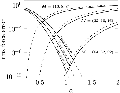
Figure 1. Achieved rms force errors (solid) for different far field cutoffs M = (2M, M, M) with M ∈ {8, 16, 32} and different near field cutoffs r_cut ∈ {4.0, 4.5, 5.0}. We also plot the estimates for the rms force error in the near field (dotted) as well as for the far field with elliptical cutoff (dashed), see Equations (28) and (31). Test case: N = 600 randomly distributed particles in a box with edge lengths L = (20, 10, 10).

For relatively large values of α as well as for large mesh sizes M, the actual error in the far field is somewhat overestimated by the derived upper bound. This is supposed to be due to the fact that the algorithm uses the full mesh ${I}$_M instead of the supposed ellipsoidal cutoff scheme. However, we see that the achieved error behavior is described very well by the stated estimates.

                                                                                                                                                                                                                                                   □

Based on the error estimates we may tune the parameters as follows. Note that a first tuning approach is discussed in Kolafa and Perram [34]. A tuning similar to Algorithm 3.1 is already used within the ScaFaCoS library [19] and can also be modified in order to tune the accuracy with respect to the absolute rms potential error, see Lindbo and Tornberg [5] for instance.

Given a near field cutoff r_cut as well as a far field cutoff M, the splitting parameter α is chosen optimal if the rms errors in the near field as well as the far field are approximately of the same size. Thus, a common approach is to solve for a given r_cut the equations

$\Delta F^{\text{S}}=\Delta {\text{F}}^{\text{L}}=\frac{\epsilon }{\sqrt{2}}$

for α and M, where the rms errors in the short range as well as the long range part are denoted by ΔF^S and ΔF^L, respectively.

Assuming that the near field and the far field part of the error are independent of each other we have

$\Delta F\approx \sqrt{{\left(\Delta F_{\approx }^{\text{S}}\right)}^2+{\left(\Delta F_{\approx }^{\text{L}}\right)}^2}\approx \sqrt{\frac{{\epsilon }^2}{2}+\frac{{\epsilon }^2}{2}}=\epsilon .$

Thus, we expect that the overall rms force error is indeed approximately of the size ε.

Algorithm 3.1 Choice of the splitting parameter α and the far field cutoff M.

Input: Box size vector L, numbers of charges N, sum of squared charge values Q, required accuracy ε > 0, near field cutoff radius 0 < r_cut ≤ min(L₁, L₂, L₃).

1. Compute α via Equation (28): Claiming $F^S\approx \epsilon \sqrt{2}$ we obtain

$\alpha =\frac{1}{r_{\text{cut}}}\sqrt{\ln \left(\frac{2\sqrt{2}Q}{\epsilon \sqrt{r_{\text{cut}}NV}}\right)}.$

2. Compute β via Equation (31): Inserting the above computed value for α we choose M such that also the far field error is approximately of the size $\epsilon \sqrt{2}$. We use the error estimate for the elliptical cutoff scheme, see Equation (31), and obtain

$\beta =\frac{\alpha }{\pi }\sqrt{\text{W}\left(\frac{2^{10}{\alpha }^2{Q}^4}{{\pi }^2{N}^2{V}^2{\epsilon }^4}\right)},$

where we denote by W(·) the well-known Lambert W function, which is implicitly defined by W(x)e^W(x) = x.

3. Set $\text{M}:\text{}\text{}=2\lceil \frac{\beta }{2}\text{L}\rceil \in 2{\mathbb{N}}^3$ (round up component wise to an even integer).

                                                                                                                                                                                                                                                  □

Given some near field cutoff radius r_cut and a required accuracy ε, the splitting parameter α and the far field cutoff M can be set via Algorithm 3.1 in order to reach the accuracy ε. Based on the used hard- and software, some specific value for r_cut will be optimal with respect to runtime. However, the computation of the long range part requires at best ${O}$(N^3∕2) arithmetic operations, see Kolafa and Perram [34, Appendix B]. In order to enable a more efficient computation we apply the NFFT algorithms, as we describe in the following section.

4. NFFT Based Fast Ewald Summation and Rms Errors

We consider the efficient evaluation of the truncated long range parts of the potentials

$\begin{array}{l}{\varphi }_{\text{t},j}^{\text{L}}:=\frac{1}{\pi V}{\displaystyle \sum _{k\in {{I}}_M}\widehat{\psi }}(k)S(k){\text{e}}^{-2\pi \text{i}(k\odot L^{-1})·x_j}\hfill \\ \approx \frac{1}{\pi V}{\displaystyle \sum _{k\in {{I}}_M}\widehat{\psi }}(k)\tilde{S}(k){\text{e}}^{-2\pi \text{i}(k\odot L^{-1})·x_j}.\hfill & (32)\end{array}$

As indicated above, the sums S(k), as given in Equation (24), can be approximated by the adjoint NFFT, $S(\text{k})\approx \tilde{S}(\text{k})$, k ∈ ${I}$_M. After a multiplication with the Fourier coefficients $\widehat{\psi }(\text{k})$ we compute the outer sums over k ∈ ${I}$_M for all j = 1, …, N via the NFFT.

The fast computation of the truncated versions of the forces' long range parts ${\text{F}}_{t,j}^L$, as defined in Equation (30), can be done in an analog manner. Note that the outer sums have then to be computed by a vector valued 3d-NFFT, i.e., three 3d-FFTs are needed. This approach is widely known as ik-differentiation since the differentiation operator ∇ is directly applied in Fourier space. We remark that the differentiation operator can instead be shifted to the window function φ, which is known as analytical differentiation and requires only the computation of one 3d-FFT in order to approximate the outer sums. However, in the present paper we only take into consideration the ik-differentiation approach.

The described method (P²NFFT) is part of the publicly available ScaFaCoS library [19]. The NFFT and the adjoint NFFT are computed by using the parallel FFT (PFFT) software [42]. See Wang et al. [43] for another implementation of the described algorithm.

Remark 4.1. Note that the NFFT as well as the adjoint NFFT are approximate algorithms. Thus, in addition to the truncation errors, see Section 3, we introduce an approximation error when applying the fast methods in Equations (24) and (32). By using the exact algorithms (NDFT and adjoint NDFT) we obtain a reference method, for which only the truncation errors in the Ewald sums are present.                                                                                                                                                                                                                                   □

The computation of the corresponding rms approximation error is done by making use of Equations (4) and (10). At first we approximate the sums S(k) by $\tilde{S}(\text{k})$ via the adjoint NFFT, which gives

$F_{\text{t},j}^{\text{L}}\approx F_{\text{nffth},j}^{\text{L}}:=\frac{2\text{i}{q}_j}{V}{\displaystyle \sum _{k\in {{I}}_M}(k\odot L^{-1})}\widehat{\psi }(k)\tilde{S}(k){\text{e}}^{-2\pi \text{i}k·(x_j\odot L^{-1})}.$

In the second step we approximate ${\text{F}}_{\mathrm{nffth},j}^L\approx {\tilde{\text{F}}}_{\mathrm{nffth},j}^L$ via a vector valued 3d-NFFT, i.e., we apply the ik-differentiation approach.

The final expression for the rms approximation error, which is valid for arbitrary window functions φ, is given in Lemma 4.2.

Lemma 4.2. Let a charge neutral system, see Equation (19), of charges q_j ∈ ℝ at positions x_j ∈ ${B}$ := L₁𝕋 × L₂𝕋 × L₃𝕋 be given. Suppose that the truncated long range parts of the forces ${\text{F}}_{t,j}^L$ as defined in Equation (30) are computed via the NFFT based method by using the oversampled mesh ${I}$_Mo and a symmetric, real valued window function φ. Then, the resulting error in the forces can for each j = 1, …, N be written in the form

$F_{\text{t},j}^{\text{L}}-{\tilde{F}}_{\text{nffth},j}^{\text{L}}=q_j{\displaystyle \sum _{\begin{array}{l}i=1\\ i\ne j\end{array}}^N{q}_i}{\chi }_{ij}.$

Thereby, the quadratic mean of the error terms χ_ij has the lower bound

${\chi }^2:=\frac{1}{V}{\displaystyle {\int }_{ℬ}\frac{1}{V}}{\displaystyle {\int }_{ℬ}{\left|{\chi }_{ij}\right|}^2}\text{d}{x}_j\text{d}{x}_i\ge {\chi }_{\text{opt}}^2,(33)$

where

$\begin{array}{l}{\chi }_{\text{opt}}^2:=\hfill \\ \frac{4}{V^2}{\displaystyle \sum _{k\in {{I}}_M}\parallel k\odot L^{-1}{\parallel }^2}\widehat{\psi }{(k)}^2\left(1-{\left[{\displaystyle \sum _{r\in {\mathbb{Z}}^3}\frac{c_{k+r\odot M_{\text{o}}}^2({\tilde{\phi }}_{\text{t}})}{c_k^2({\tilde{\phi }}_{\text{t}})}}\right]}^{-2}\right).\hfill & (34)\end{array}$

The corresponding optimal NFFT deconvolution coefficients are given by Equation (8). If the deconvolution coefficients are set as in Equation (6), the expected quadratic error χ² reads as

${\chi }_{\text{std}}^2:=\frac{4}{V^2}\text{}{\displaystyle \sum _{k\in {{I}}_M}\parallel k\odot L^{-1}{\parallel }^2}\widehat{\psi }{(k)}^2\left({\left[{\displaystyle \sum _{r\in {\mathbb{Z}}^3}\text{}}\frac{c_{k+r\odot M_{\text{o}}}^2({\tilde{\phi }}_{\text{t}})}{c_k^2({\tilde{\phi }}_{\text{t}})}\right]}^2\text{}-1\right)\text{}.(35)$

Proof. For the sake of completeness we present a short sketch of the proof. We can write the error ${\text{F}}_{t,j}^L-{\tilde{\text{F}}}_{\mathrm{nffth},j}^L$ as

$\begin{array}{l}{F}_{\text{t},j}^{\text{L}}-{\tilde{F}}_{\text{nffth},j}^{\text{L}}=\left(F_{\text{t},j}^{\text{L}}-F_{\text{nffth},j}^{\text{L}}\right)+\left(F_{\text{nffth},j}^{\text{L}}-{\tilde{F}}_{\text{nffth},j}^{\text{L}}\right)\hfill \\ =q_j{\displaystyle \sum _{i=1}^N{q}_i}{\chi }_{ij}.\hfill & (36)\end{array}$

If the window function φ is symmetric, one easily finds that χ_jj = 0. In order to obtain a representation of χ_ij we have to apply the error formula of the adjoint NFFT, see Equation (10), to S(k) and compute the first part ${\text{F}}_{t,j}^L-{\text{F}}_{\mathrm{nffth},j}^L$.

In the second part we apply the representation of the computed NFFT approximation, see Equation (2), in order to compute ${\tilde{\text{F}}}_{\mathrm{nffth},j}^L$ or rather ${\text{F}}_{\mathrm{nffth},j}^L-{\tilde{\text{F}}}_{\mathrm{nffth},j}^L$.

Putting everything together, we obtain a representation for χ_ij and can compute the integral as given in Equation (33), where the integration domain ${B}$ is defined as ${B}$ := L₁𝕋 × L₂𝕋 × L₃𝕋. We finally obtain

$\begin{array}{l}{\chi }^2=\frac{4}{V^2}{\displaystyle \sum _{k\in {{I}}_M}\parallel k\odot L^{-1}{\parallel }^2}\widehat{\psi }{(k)}^2{\left|1-{\widehat{d}}_k^2{c}_k^2({\tilde{\phi }}_{\text{t}})\right|}^2\hfill \\ -\frac{4}{V^2}{\displaystyle \sum _{k\in {{I}}_M}\parallel k\odot L^{-1}{\parallel }^2}\widehat{\psi }{(k)}^2{\widehat{d}}_k^4{c}_k^4({\tilde{\phi }}_{\text{t}})\hfill \\ +\frac{4}{V^2}{\displaystyle \sum _{k\in {{I}}_M}\parallel k\odot L^{-1}{\parallel }^2}\widehat{\psi }{(k)}^2{\left({\displaystyle \sum _{r\in {\mathbb{Z}}^3}{\widehat{d}}_k^2}{c}_{k+r\odot M_{\text{o}}}^2({\tilde{\phi }}_{\text{t}})\right)}^2.\hfill & (37)\end{array}$

Minimizing with respect to ${\widehat{d}}_{\text{k}}$ for each k provides the optimal coefficients

${\widehat{d}}_k:=\frac{c_k({\tilde{\phi }}_{\text{t}})}{{\displaystyle \sum _{r\in {\mathbb{Z}}^3}{c}_{k+r\odot M_{\text{o}}}^2}({\tilde{\phi }}_{\text{t}})},$

i.e., we have to optimize the NFFT algorithms with respect to the error in the ${L}$₂-norm. The expressions given in Equations (35) and (34) are obtained by inserting ${\widehat{d}}_{\text{k}}=c_{\text{k}}^{-1}({\tilde{\phi }}_{\text{t}})$ and the computed optimal coefficients into Equation (37), respectively.                                                                                                              ◼

We denote by

$\Delta F_{\text{fast}}^{\text{L}}:=\sqrt{\frac{1}{N}{\displaystyle \sum _{j=1}^N{\Vert F_{\text{t}}^{\text{L}}-{\tilde{F}}_{\text{nffth},j}^{\text{L}}\Vert }^2}}\approx \frac{\chi Q}{\sqrt{N}}(38)$

the resulting RMS error.

Remark 4.3. Note the difference to the derivation of the optimal influence function by Hockney and Eastwood [1, Section 8-3-3]. The optimal influence function is derived via considering the approximation of the non truncated Fourier space sums, see Equation (26), by transforming the continuous charge distribution into a grid based charge density. In contrast, we already start with the truncated sum over k ∈ ${I}$_M.

The two deconvolution steps and multiplication with the Fourier coefficients are summarized as the so called influence function in the P³M framework. The resulting optimal rms force error in the case of ik-differentiation reads as

$\frac{4}{V^2}{\displaystyle \sum _{k\in {{I}}_M}\left({\displaystyle \sum _{s\in {\mathbb{Z}}^3}{\left|R(k+s\odot M)\right|}^2}-\frac{{\left|\text{i}{(k\odot L^{-1})}^{\top }{\displaystyle \sum _{s\in {\mathbb{Z}}^3}{c}_{k+s\odot M}^2}({\tilde{\phi }}_{\text{t}})R(k+s\odot M)\right|}^2}{\parallel k\odot L^{-1}{\parallel }^2{\left({\displaystyle \sum _{r\in {\mathbb{Z}}^3}{c}_{k+r\odot M}^2}({\tilde{\phi }}_{\text{t}})\right)}^2}\right)},(39)$

where $\text{R}(\text{k}):=-\frac{i(\text{k}\odot {\text{L}}^{-1})}{\left|\right|\text{k}\odot {\text{L}}^{-1}|{|}^2}{e}^{-{\pi }^2\left|\right|\text{k}\odot {\text{L}}^{-1}|{|}^2∕{\alpha }^2}$, see Hockney and Eastwood [1, Eq. 8-23]. Note that the single summands tend to zero exponentially fast and thus we may only consider the contributions for s = 0, for which we obtain Equation (34). This shows the mathematical equivalence of the P³M and the P²NFFT method in the case that we choose the oversampling factor σ = (1, 1, 1). Note that the two methods provide additional features, such as analytic differentiation and interlacing, which can further improve the performance, see [1, 3, 20, 44] for instance. We remark that the formulas of the P³M rms errors as well as for the optimal influence functions are valid for arbitrary window functions as well and that analogical error estimates are also known for the analytic differentiation approach, see Hockney and Eastwood [1] and Pippig [20]. The window function is called charge assignment function in terms of the P³M, for which usually B-splines are used. The order of the B-spline 2m is named charge assignment order. Correspondingly, the convolutions in spatial and Fourier domains are known as charge assignment on and from the grid, respectively.                                                                                                                                                                                                □

4.1. Efficient Computation of the Resulting Rms Errors

In the following we discuss how the above derived expressions for the rms force error can be estimated efficiently. In three dimensions we use a tensor product approach, see Equation (3), in order to construct the window function φ by only using univariate functions.

Thus, also the Fourier coefficients $c_{\text{k}}({\tilde{\phi }}_t)$, k ∈ ℤ³, are of a tensor product structure

$c_k({\tilde{\phi }}_{\text{t}})={\displaystyle \prod _{j=1}^3{c}_{k_j}}({\tilde{\phi }}_{j,\text{t}}).$

In order to estimate the rms force error efficiently we separate the computations regarding the three dimensions by using an approximation of the form

$\frac{1}{x}\approx {\displaystyle \sum _{i=1}^n{r}_i}{\text{e}}^{-w_{i}x}\text{ for }x\in [1,\ell ),(40)$

where ℓ ≫ 1 should be chosen large enough. Such an approximation can be obtained with the help of the well-known ESPRIT algorithm [45], see Potts and Tasche [46] for instance, or by using the Remez algorithm, which has been applied by Hackbusch [47].

For k ∈ ${I}$_M and L_max := max{L₁, L₂, L₃} we have

$1\le x:=L_{\max }^2\Vert k\odot L^{-1}{\Vert }^2\text{}\le L_{{\max }^2}\text{}\left(\frac{M_1^2}{4L_1^2}+\frac{M_2^2}{4L_2^2}\text{}+\text{}\frac{M_3^2}{4L_3^2}\right)=\frac{3{\beta }^2{L}_{\max }^2}{4}.$

Thus, we should choose $\ell \ge L_{max}^2\left(\frac{M_1^2}{4L_1^2}+\frac{M_2^2}{4L_2^2}+\frac{M_3^2}{4L_3^2}\right)$.

Example 4.4. For cubic box shapes, i.e., L := (L, L, L) and M := (M, M, M) we have

$L_{\max }^2\Vert k\odot L^{-1}{\Vert }^2\le \Vert k{\Vert }^2\le \frac{3M^2}{4}<2·{10}^5\forall M\le 512,$

which is supposed to suffice if small particle systems are considered. In Hackbusch [47] the authors provide an approximation with only n = 11 exponential terms with

${\max }_{x\in [1,2·{10}^5)}\left|\frac{1}{x}-{\displaystyle \sum _{i=1}^{11}{r}_i}{\text{e}}^{-w_{i}x}\right|\le 7·{10}^{-6}.$

                                                                                                                                                                                                                                                   □

Now we have for k ≠ 0

$\begin{array}{l}\Vert k\odot L^{-1}{\Vert }^2\widehat{\psi }{(k)}^2\hfill \\ =\frac{{\text{e}}^{-2{\pi }^2\Vert k\odot L^{-1}{\Vert }^2/{\alpha }^2}}{\Vert k\odot L^{-1}{\Vert }^2}\hfill \\ =\frac{L_{\max }^2{\text{e}}^{-2{\pi }^2\Vert k\odot L^{-1}{\Vert }^2/{\alpha }^2}}{\frac{L_{{\max }^2}k{1}^2}{L_1^2}+\frac{L_{{\max }^2}k{2}^2}{L_2^2}+\frac{L_{{\max }^2}k{3}^2}{L_3^2}}\hfill \\ \approx L_{{\max }^2}{\displaystyle \sum _{i=1}^n{r}_i}{\text{e}}^{-(2{\pi }^2/{\alpha }^2+w_i{L}_{{\max }^2})(k_1^2/L_1^2+k_2^2/L_2^2+k_3^2/L_3^2)}.\hfill & (41)\end{array}$

For the window functions as presented in Section 2 we have

${\displaystyle \sum _{r\in \mathbb{Z}\setminus \left\{0\right\}}\frac{c_{k+r{\sigma }_j{M}_j}^2({\tilde{\phi }}_{j,\text{t}})}{c_k^2({\tilde{\phi }}_{j,\text{t}})}}\{\begin{array}{ll}\le s_j(k)\hfill & :\phi \in \{\text{B-Spline},\text{Bessel}\},\hfill \\ \approx s_j(k)\hfill & :\phi \in \left\{\text{Gaussian}\right\},\hfill \end{array}(42)$

where k ∈ ${I}$_Mj, see Equations (12), (16), (17). Then

${\left({\displaystyle \sum _{r\in \mathbb{Z}}\frac{c_{k+r{\sigma }_j{M}_j}^2({\tilde{\phi }}_{j,\text{t}})}{c_k^2({\tilde{\phi }}_{j,\text{t}})}}\right)}^2\approx 1+2s_j(k)+s_j^2(k)=\text{}\text{}:1+{\tilde{s}}_j(k)$

and for k = (k₁, k₂, k₃) ∈ ${I}$_M we obtain

$\begin{array}{l}{\left[{\displaystyle \sum _{r\in {\mathbb{Z}}^3}\frac{c_{k+r\odot M_{\text{o}}}^2({\tilde{\phi }}_{\text{t}})}{c_k^2({\tilde{\phi }}_{\text{t}})}}\right]}^2\approx \hfill \\ 1+{\displaystyle \sum _{j=1}^3{\tilde{s}}_j}(k_j)+{\displaystyle \sum _{j_1<j_2}{\tilde{s}}_{j_1}}(k_{j_1}){\tilde{s}}_{j_2}(k_{j_2})+{\displaystyle \prod _{j=1}^3{\tilde{s}}_j}(k_j).\hfill & (43)\end{array}$

For i = 1, …, n and j = 1, …, 3 we define the sums

$\begin{array}{l}{S}_{i,j}^{\text{std}}:={\displaystyle \sum _{k\in {{I}}_{M_j}}{\text{e}}^{-(2{\pi }^2/{\alpha }^2+w_i{L}_{{\max }^2})k^2/L_j^2}}\hfill \\ R_{i,j}^{\text{std}}:={\displaystyle \sum _{k\in {{I}}_{M_j}}{\tilde{s}}_j}(k){\text{e}}^{-(2{\pi }^2/{\alpha }^2+w_i{L}_{{\max }^2})k^2/L_j^2}\hfill \\ S_{i,j}^{\text{opt}}:={\displaystyle \sum _{k\in {{I}}_{M_j}}\frac{1}{1+{\tilde{s}}_j(k)}}{\text{e}}^{-(2{\pi }^2/{\alpha }^2+w_i{L}_{{\max }^2})k^2/L_j^2}\hfill \\ R_{i,j}^{\text{opt}}:={\displaystyle \sum _{k\in {{I}}_{M_j}}\frac{{\tilde{s}}_j(k)}{1+{\tilde{s}}_j(k)}}{\text{e}}^{-(2{\pi }^2/{\alpha }^2+w_i{L}_{{\max }^2})k^2/L_j^2}\hfill \end{array}$

and obtain for ${\chi }_{\mathrm{std}}^2$, as defined in Equation (35), by applying Equation (41)

$\begin{array}{ll}{\chi }_{\text{std}}^2\approx \frac{4}{V^2}{\displaystyle \sum _{k\in {{I}}_M}\Vert k\odot L^{-1}{\Vert }^2}\widehat{\psi }{\left(k\right)}^2\left({\displaystyle \prod _{j=1}^3\left[1+{\tilde{s}}_j(k_j)\right]}-1\right)& (44)\end{array}$

$\begin{array}{l}\approx \frac{4L_{{\max }^2}}{V^2}{\displaystyle \sum _{i=1}^n{r}_i}({\displaystyle \sum _{j_1,j_2,j_3}\left(S_{i,j_1}^{\text{std}}{S}_{i,j_2}^{\text{std}}{R}_{i,j_3}^{\text{std}}+S_{i,j_1}^{\text{std}}{R}_{i,j_2}^{\text{std}}{R}_{i,j_3}^{\text{std}}\right)}\\ +R_{i,1}^{\text{std}}{R}_{i,2}^{\text{std}}{R}_{i,3}^{\text{std}})\end{array}$

$\begin{array}{ll}-\frac{4L_{{\max }^2}}{V^2}\left({\displaystyle \prod _{j=1}^3\left[1+{\tilde{s}}_j\left(0\right)\right]}-1\right){\displaystyle \sum _{i=1}^n{r}_i},& (45)\end{array}$

i.e., we can estimate the error with ${O}$(n(M₁ + M₂ + M₃)) arithmetic operations.

Similarly, we obtain the following estimate for the optimal error ${\chi }_{\mathrm{opt}}^2$, see Equation (34).

$\begin{array}{l}{\chi }_{\text{opt}}^2\approx \frac{4}{V^2}{\displaystyle \sum _{k\in {{I}}_M}\Vert k\odot L^{-1}{\Vert }^2}\widehat{\psi }{\left(k\right)}^2\left(1-{\displaystyle \prod _{j=1}^3\frac{1}{1+{\tilde{s}}_j(k_j)}}\right)\hfill \\ =\frac{4}{V^2}{\displaystyle \sum _{k\in {{I}}_M}\Vert k\odot L^{-1}{\Vert }^2}\widehat{\psi }{\left(k\right)}^2{\displaystyle \prod _{j=1}^3\frac{1}{1+{\tilde{s}}_j(k_j)}}·\hfill \\ \left({\displaystyle \prod _{j=1}^3\left[1+{\tilde{s}}_j(k_j)\right]}-1\right)\hfill \\ \approx \frac{4L_{{\max }^2}}{V^2}{\displaystyle \sum _{i=1}^n{r}_i}({\displaystyle \sum _{j_1,j_2,j_3}(S_{i,j_1}^{\text{opt}}{S}_{i,j_2}^{\text{opt}}{R}_{i,j_3}^{\text{opt}}+S_{i,j_1}^{\text{opt}}{R}_{i,j_2}^{\text{opt}}{R}_{i,j_3}^{\text{opt}})}\hfill \\ +R_{i,1}^{\text{opt}}{R}_{i,2}^{\text{opt}}{R}_{i,3}^{\text{opt}})\hfill \\ -\frac{4L_{{\max }^2}}{V^2}\left(1-{\displaystyle \prod _{j=1}^3\frac{1}{1+{\tilde{s}}_j(0)}}\right){\displaystyle \sum _{i=1}^n{r}_i}.\hfill & (46)\end{array}$

Remark 4.5. With M = βL we have

$\begin{array}{l}\frac{1}{V}\frac{{\text{e}}^{-{\pi }^2\Vert k\odot L^{-1}{\Vert }^2/{\alpha }^2}}{\Vert k\odot L^{-1}{\Vert }^2}=\frac{{\beta }^3}{M_1{M}_2{M}_3}\frac{{\text{e}}^{-{\pi }^2\Vert k\odot M^{-1}{\Vert }^2/({\alpha }^2{\beta }^2)}}{\frac{1}{\beta }\Vert k\odot M^{-1}\Vert }\hfill \\ =\frac{{\beta }^4}{\left|{{I}}_M\right|}\frac{{\text{e}}^{-{\pi }^2\Vert k\odot M^{-1}{\Vert }^2/({\alpha }^2{\beta }^2)}}{\Vert k\odot M^{-1}\Vert }\hfill & (47)\end{array}$

and additionally the error sums as defined in Equation (11) only depend on the values $\raisebox{1ex}{$k$}\!\left/ \!\raisebox{-1ex}{$\sigma M$}\right.\in \left[0,\raisebox{1ex}{$1$}\!\left/ \!\raisebox{-1ex}{$2\sigma $}\right.\right]$. Thus, the errors χ_std∕opt are supposed to be almost equal among particle systems with the same charge and particle density, if β, α as well as the NFFT parameters m, σ and b are kept constant.

In other words, the errors can be predicted by considering a smaller particle system, which is scaled appropriately (see [48, Section 5]), where the same approach has been applied. We give an example in Table 1, where we list the approximated errors obtained via Equation (45) as well as by using Equation (44), for which the second approximation for the separation of the single dimensions, see Equation (40), is not applied.

TABLE 1

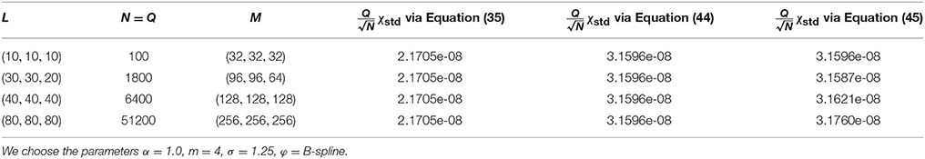
Table 1. Computed values for Equations (35), (44), and (45) for different systems having the same particle and charge density (see the supposed values for L, N, and Q).

Note that the error as given in Equation (35) can be computed exactly in case of the B-spline window, since the one dimensional sums over r_j ∈ ℤ can be expressed in terms of the Euler-Frobenius polynomials, see Nestler [30] and references therein. However, this approach is numerically unstable since the sums take values very close to 1. Thus, in order to get a value for the exact error given in Equation (35) we compute the aliasing sums over r_j ∈ ℤ \ {0}, see Equation (12), directly via truncation. Note that the summands tend to zero like ${O}(r_j^{-4m})$.                                                                                                                                                  □

4.2. Comparison between Different Window Functions

We consider the window functions from Section 2 and evaluate the occurrent rms errors, as described above, for some test scenarios.

In the following examples we consider a particle system containing N = 300 randomly distributed charges $q_j={(-1)}^j$ distributed in a cubic box with edge length 10, i.e., L = (L, L, L) = (10, 10, 10). We compute the quadratic means χ_std as well as χ_opt via Equations (45) and (46), respectively, for different values of the splitting parameter α and compare the predicted errors with measured errors. For this purpose we apply the P²NFFT implementation in ScaFaCoS [19] and set r_cut := 0 in order to compute only the far field. The exact computation is done by applying the NDFT algorithms instead of the NFFT methods, see Remark 4.1. Note that the P²NFFT is based on the standard deconvolution approach, see Equation (6).

4.2.1. B-Spline Window

For the B-spline window the upper bounds s_j(k), as introduced by Equation (42), are given in Equation (12).

Example 4.6. The results for the B-spline window function are plotted in Figure 2. We see that the measured errors are estimated very precisely by χ_std and that the usage of the optimized deconvolution approach does, especially in the range of high precisions, not promise significant improvements, which is due to the rapid decrease of the Fourier coefficients ψ(k).                                                                                                                                                                                     □

FIGURE 2

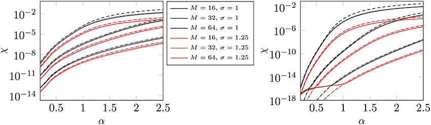
Figure 2. Approximate values for χ_opt via Equation (46) (dotted) and χ_std via Equation (45) (dashed) for different far field cutoffs M with respect to the splitting parameter α. Thereby we choose the support parameter m = 3 (left) and m = 6 (right) as well as the oversampling factor α ∈ {1, 1.25} (see legend). The corresponding measured errors χ_std are represented by the solid lines. (Window function: B-spline).

4.2.2. Bessel Window

For the Bessel I₀ window the upper bounds s_j(k) for k ∈ ${I}$_Mj are given in Equation (16). We claim that the accuracy of the P²NFFT method can be improved significantly by tuning the shape parameter b.

Example 4.7. We give an example on how the choice of the shape parameter b influences the accuracy of our method and compute χ_std for different values of b := (b, b, b), where we set α := 0.8, M := (32, 32, 32), σ := (1, 1, 1) and m := 3. The results are plotted in Figure 3.

FIGURE 3

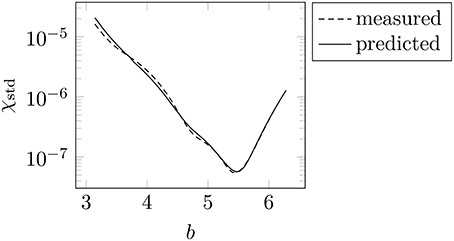
Figure 3. Predicted and measured errors χ_std for different values of the shape parameter b := (b, b, b). We choose the parameters α = 0.8, M = (32, 32, 32), σ = (1, 1, 1) and m = 3. (Window function: Bessel).

For typical scenarios we suppose that the error behaves as depicted in Figure 3, that is, that the error adopts its minimum for some optimal value b = b_opt and grows with increasing distance |b − b_opt| from the optimal value.

In this specific example we obtain b_opt ≈ 5.5. Note that the choice of the standard shape parameter $b:=b_0=(2\sigma -1)\frac{\pi }{\sigma }=\pi$ results in an increase of the error by more than two orders of magnitude. In other words, an appropriate method to tune the shape parameter seems necessary.                                                                                                                                                                                                                                  □

We suggest the following approach to tune the shape parameter b automatically, cf. Nestler [30]. For simplicity we assume that approximately the same oversampling factor σ is applied in all three dimensions, i.e., we set σ := (σ, σ, σ), where σ ≥ 1.

Thus, it is reasonable to use also the same shape parameter b > 0 in the single dimensions, i.e., we set b := (b, b, b). Note that the oversampled grid size has to be set via $M_{\text{o},j}:\text{}\text{}=2\lceil \frac{\sigma }{2}{M}_j\rceil ,$ since we need ${\text{M}}_o\in 2{\mathbb{N}}^3$. Thus, the oversampling factors σ_j := M_{o, j} ∕ M_j, which are actually applied in the single dimensions, may slightly differ from σ.

In Algorithm 4.1 we denote by χ(b, m, σ) the predicted rms error terms χ_opt and χ_std, which actually depend on the chosen shape parameter b, the support parameter m, the oversampling factor σ as well as the applied deconvolution scheme. Based on the given sets of parameters the resulting error terms χ can be approximated by Equations (45) and (46), respectively.

Algorithm 4.1 (Shape parameter tuning).

Input: Splitting parameter α, box size vector L, far field cutoff M, support parameter m, oversampling factor σ, which is to be applied in all three dimensions.

(i) Set b_opt := b₀, i.e., take the standard shape parameter, see Equation (14), as a first guess for the optimal shape parameter.

(ii) Choose a start step size d, e.g., $d:=\frac{b_{\mathrm{opt}}}{2}$.

(iii) Set b_opt := argmin_{b∈{bopt−d, bopt, bopt+d}} χ(b, m, σ).

If the old and the new value for b_opt coincide, set $d:\text{}\text{}=\raisebox{1ex}{$d$}\!\left/ \!\raisebox{-1ex}{$2$}\right.$.

(iv) Repeat (iii) until the computed optimal error does not significantly change anymore.

Output: Optimal shape parameter b_opt and the best possible error χ_min.                                                                                                                                                                                                                               □

Example 4.8. We tune the shape parameter b, which is applied in all three dimensions, by the suggested tuning Algorithm 4.1 and plot the results for the Bessel window function in Figure 4. As already observed for the B-spline window, we cannot see significant differences between χ_opt as well as χ_std.

FIGURE 4

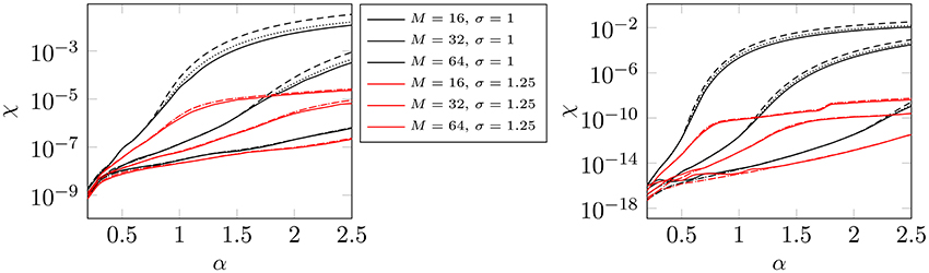
Figure 4. Approximate values for χ_opt via Equation (46) (dotted) and χ_std via Equation (45) (dashed) for different far field cutoffs M with respect to the splitting parameter α. Thereby we choose the support parameter m = 3 (left) and m = 6 (right) as well as the oversampling factor σ ∈ {1, 1.25} (see legend). The corresponding measured errors (χ_std) are represented by the solid lines. (Window function: Bessel).

The default values for the shape parameter are

$b_0=\{\begin{array}{ll}\pi \approx 3.14\hfill & :\sigma =1,\hfill \\ \frac{6}{5}\pi \approx 3.77\hfill & :\sigma =\mathrm{1.25.}\hfill \end{array}$

In Figure 5 we plot the tuned optimal shape parameters b_opt for the parameter setting m = 3, M = 32. We also compare the errors obtained by using the tuned optimal shape parameter b_opt with the results obtained by setting b = b₀. Obviously, the optimal value b_opt very much depends on the applied splitting parameter α, which determines how fast the Fourier coefficients $\widehat{\psi }(\text{k})$ are decreasing. We obtain significantly smaller approximation errors by using the tuned shape parameters.                                                                                                                                                                                                                               □

FIGURE 5

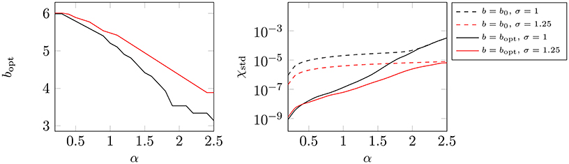
Figure 5. Optimal shape parameters b_opt (left) for the setting m = 3, M = 32, where σ = 1 (black) and σ = 1.25 (red). On the right hand side we plot the measured errors χ_std, which were obtained with b = b_opt (solid) and with b = b₀ (dashed), respectively. (Window function: Gaussian).

4.2.3. Gaussian Window

For the Gaussian window function we set s_j(k) via Equation (17), i.e., we do not compute upper bounds of the underlying error sums but rather approximations. Note that in addition the computation of $c_k({\tilde{\phi }}_{j,t})$ is numerically unstable for large k. In other words, we expect that the error prediction is not as precise as for B-splines or the Bessel window. The shape parameter can be tuned via Algorithm 4.1, too.

Example 4.9. The results for the Gaussian window function, which were obtained with the optimal shape parameters found by Algorithm 4.1, are plotted in Figure 6. As for the Bessel window we obtain considerably different optimal shape parameters b_opt among different values of the splitting parameter α.

FIGURE 6

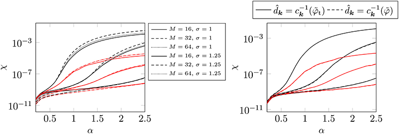
Figure 6. LHS: Approximate values for χ_opt via Equation(46)(dotted) and χ_std via Equation(45)(dashed) for for different far field cutoffs M with respect to the splitting parameter α. Thereby we choose the support parameter m = 6 as well as the oversampling factor σ ∈ {1, 1.25}. The corresponding measured errors (χ_std) are represented by the solid lines. RHS: We compare the results obtained by setting ${\widehat{d}}_{\text{k}}=c_{\text{k}}^{-1}(\widetilde{{\phi }_t})$ with those obtained by applying ${\widehat{d}}_{\text{k}}=c_{\text{k}}^{-1}(\tilde{\phi })$. (Window function: Gaussian).

Since the estimation of the underlying error sums is easier in the case that the Fourier coefficients of the truncated Gaussian are used, we use these coefficients within the deconvolution steps of the NFFT and the adjoint NFFT. For the evaluation of the complex valued error function within ScaFaCoS [19] we use the libcerf library [49]. We can see that the errors are predicted fairly well for relatively large splitting parameters α. For smaller values of α we obtain somewhat inaccurate results, which is due to the above described problems connected with the complex valued error function.

We suppose that we cannot considerably profit from using the Fourier coefficients of the truncated Gaussian $c_{\text{k}}(\widetilde{{\phi }_t})$ since the coefficients $\widehat{\psi }(\text{k})$ tend to zero exponentially fast in k. Indeed, we obtain almost the same errors by using the Fourier coefficients of the non-truncated Gaussian $c_{\text{k}}(\tilde{\phi })$ instead, see right hand side in Figure 6.                                                                                                                                                                                                                                     □

4.2.4. Comparison

In order to compare the three different window functions we plot some of the predicted errors χ_std, as presented in the Examples above, in Figure 7.

FIGURE 7

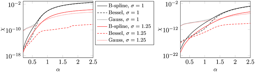
Figure 7. Predicted errors χ_std as presented in Examples 4.6, 4.8, and 4.9 for the support parameter m = 6, where M = 16 (left) and M = 32 (right), respectively.

The Bessel window function provides the most accurate results in most cases. It can be seen that the B-Spline performs best in terms of accuracy only for very small values of α. In this case the coefficients $\widehat{\psi }(\text{k})$ tend to zero very rapidly, i.e., the error is strongly dominated by the terms k ≈ 0 and thus the B-spline profits from the fact that s_j(k) → 0 as k → 0, see Equation (12).

It seems that the Gaussian can not keep up with the B-spline and the Bessel window function in terms of accuracy. Note that the PNFFT software [50] allows the usage of a third order interpolation scheme for the repeated evaluation of the window function. In three dimensions the window function is constructed based on a tensor product approach, i.e., the interpolation can be restricted to the single dimensions. This enables an efficient and highly accurate evaluation, which is independent from the used window function. The evaluation of the window function only consists of a few arithmetical operations, which is in terms of computational costs similar to the fast Gaussian gridding [26], if the Gaussian window function is used.

Based on the presented comparison we suppose that, depending on the required accuracy, the B-spline or the Bessel window function will be most profitable in terms of efficiency. Thus, we restrict our considerations to these two window functions in the following examples.

4.3. Parameter Tuning and Numerical Examples

We recall Remarks 3.1, 3.2, and 4.5, which show that the predicted errors are of a comparable size among particle systems with the same particle and charge density, if the FFT mesh size is scaled appropriately. Thus, we can tune all parameters of our fast algorithm for a small particle system and apply the tuned sets of parameters also to larger systems while keeping the performance of the algorithm in terms of accuracy as well as efficiency.

4.3.1. Choice of the Oversampling Factor

The accuracy of the P²NFFT method strongly depends on the properties of the window function. We obtain more accurate results by using a larger support parameter m, for instance. In addition, we can apply oversampling in order to increase the accuracy of the algorithm. We aim to choose the oversampling factor σ as large as necessary in order to reach a certain accuracy. In the end, different combinations of the parameters m and σ will be possible, of which one will be optimal in terms of runtime.

With the help of the error estimates, as presented above, we are able to tune the oversampling factor for a given mesh size M and support parameter m. For simplicity we again assume that approximately the same oversampling factor is applied in all three dimensions, i.e., we have σ ≈ (σ, σ, σ) with σ ≥ 1.

Given some near field cutoff r_cut and a required accuracy ε, the Ewald summation parameters α and β can be determined via Algorithm 3.1. Note that finally the actual optimal splitting parameter will slightly differ from the computed one, since the approximations via NFFT and adjoint NFFT introduce additional aliasing errors.

However, the NFFT parameters are tuned in order to fulfill

$\Delta F_{\text{fast}}^{\text{L}}\le {\epsilon }_2\le \frac{\epsilon }{\sqrt{2}},(48)$

i.e., we force the approximation error $\Delta F_{\mathrm{fast}}^L$ as defined in Equation (38) to be less or equal to the Ewald type rms errors in the near field as well as in the far field. Then, we suppose that the NFFT approximation errors are small enough such that the required accuracy ε is still achieved.

We apply a simple binary search algorithm in order to tune the required oversampling factor, see Algorithm 4.2.

Algorithm 4.2 (Tune the oversampling factor).

Input: support parameter m, Ewald parameter α, NFFT mesh size M, box length vector L, required accuracy ε₂.

(i) Define a maximum oversampling factor σ_max, e.g., σ_max := 2. If the resulting error $\Delta F_{\mathrm{fast}}^L({\sigma }_{\max })>{\epsilon }_2$, then set σ_min := σ_max.

(ii) Else: If $\Delta F_{\mathrm{fast}}^L(1)\le {\epsilon }_2$, then set σ_min := 1.

(iii) Else: Set $\sigma :=\frac{1}{2}(1+{\sigma }_{\max })$ and use a simple binary search method to approximately solve $\Delta F_{\mathrm{fast}}^L(\sigma )={\epsilon }_2$ for σ.

Output: required oversampling factor σ_min ∈ [1, σ_max]. If the required accuracy ε₂ cannot be achieved, we simply return σ_max.

                                                                                                                                                                                                                                                 □

In the following examples we apply Algorithm 4.2 in order to tune σ for different parameter settings. Thereby, we set σ_max := 2 and compute the oversampling factor with an absolute accuracy of 10⁻². Note that especially for small mesh sizes M the actual oversampling factor, which is finally applied in each dimension, will slightly differ from the tuned value, since we need ${\text{M}}_{\text{o}}\in 2{\mathbb{N}}^3$. But, since we aim to tune the oversampling factor for relatively small mesh sizes in order to apply the same parameter also to larger systems, cf. Remarks 3.2 and 4.5, it is reasonable to tune σ with respect to a higher precision.

The required accuracy ε₂ is set to

${\epsilon }_2:=\frac{\epsilon }{\sqrt{2}},$

i.e., we want that the approximation errors in the long range part are approximately of the same size than the truncation errors in the near field as well as the far field. We can actually not prove that this approach will always force the overall rms force error to be smaller than ε. However, the truncation error in the far field, see Example 3.3, is always overestimated since the algorithm uses the full mesh ${I}$_M instead of a radial cutoff scheme and additionally the mesh size M has been computed by rounding above to the next even integer, see step 3 in Algorithm 3.1. Moreover, also the NFFT approximation errors are supposed to be somewhat smaller than predicted. Thus, we still suppose that the required accuracy can be reached, see Example 4.10 for instance.

In the following examples we consider again the particle system as introduced in Section 4.2. In Example 4.12 we consider also larger systems.

Example 4.10. For different values of the near field cutoff radius r_cut we tune the Ewald parameters α and β with Algorithm 3.1 in order to reach the accuracy ε = 10⁻⁸. In order to tune the NFFT parameters we claim Equation (48) to be fulfilled.

For different values of the support parameter m we tune the oversampling factor σ by applying Algorithm 4.2 for the B-spline window. The tuned parameters as well as the achieved rms force errors ΔF and the measured computation times t are listed in Table 2. The corresponding results, where we use no oversampling (σ := 1) are given in Table 3. Note that the required accuracy may for no m ∈ ℕ be reached, see Equation (13).

TABLE 2

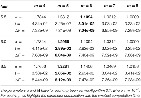
Table 2. Tuned oversampling factors σ_min, achieved computation times t in seconds and measured rms force errors ΔF for the B-spline window.

TABLE 3

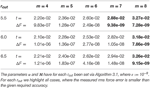
Table 3. Measured computation times t in seconds as well as achieved rms force errors ΔF for the B-spline window without oversampling, i.e., σ = 1.0.

We can see that it is in general more favorable in terms of computational costs to use a B-spline with a smaller support parameter m combined with spending some oversampling. As an example, in the case r_cut = 6, we need m ≥ 8 in order to reach the required accuracy, if we do not use oversampling. With an oversampling factor σ ≈ 1.3 we can reduce the computational costs since already the support parameter m = 5 is sufficient.

The presented runtimes include the computation of the potentials as well as the forces and have been measured on an Intel i5-2400 single core processor that runs on 3.10 GHz with 8 GB main memory. The software was built with the Gnu C Compiler at version 4.7.1 and optimization flags “-O3”. For the repeated evaluation of the window function we use a third order interpolation scheme based on interpolation tables instead of evaluating the functions directly. Thus, the speed of the evaluation is independent from the used window function, as already mentioned above. We stress that it may strongly depend on the used hardware, compiler and the like, which parameter setting is optimal regarding the required runtime. Note that the P²NFFT framework also enables the computation of the particle interactions on massively parallel architectures, which will also change the optimal parameters.

In Table 4 we list the tuned parameters as well as achieved rms force errors and runtimes for the Bessel window. For small values of the support parameter m the B-spline window requires less oversampling in order to reach the required accuracy. In contrast, for m ≥ 6 the Bessel window function demands less or equal oversampling. We achieve even smaller computation times than for the B-spline window.                                                                                                                                                                                                                                      □

TABLE 4

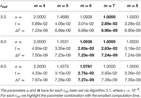
Table 4. Tuned oversampling factors σ_min, achieved computation times t in seconds and measured rms force errors ΔF for the Bessel window.

4.3.2. Runtime Over r_cut

In addition to the above described parameter tuning, for which the near field cutoff r_cut has to be specified, we also want to tune the parameter r_cut in order to achieve an (almost) optimal runtime. For small particle systems we may apply the above described tuning for different values of r_cut and compare the achieved runtimes.

Example 4.11. We tune the parameters as described in the previous considerations for different near field cutoffs r_cut, compare to Example 4.10. Thereby, we again choose ε := 10⁻⁸ and plot the measured runtimes over r_cut in Figure 8. Note the unexpected jumps in the runtime plots, which result from an increased FFT computation time in the long range part, if the oversampled grid size shows an unprofitable decomposition into prime factors.

FIGURE 8

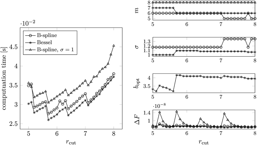
Figure 8. Measured runtimes for different values of r_cut (left). The required rms force accuracy was set to ε := 10⁻⁸. The parameters (right) were chosen by applying Algorithms 3.1, 4.1, and 4.2. For each r_cut we considered different combinations of m and σ, where we chose the one yielding the smallest computation time. Test case: N = 300 randomly distributed particles, box size: 10 × 10 × 10.

The corresponding tuned parameters and the achieved rms force errors can be found in Figure 8 as well. Note that we also consider the case σ = 1 for the B-spline window, where for each r_cut we choose the support parameter m ≤ 8 as small as possible, i.e., we increase m ≤ 8 step by step until the predicted error $\Delta F_{\text{fast}}^{\text{L}}$ for σ = 1 is smaller than ε₂, cf. Equation (48). In some cases the requested precision could not be achieved. Again, note that the accuracy may also not be achieved for larger support parameters m, cf. Equation (13). In contrast, the required accuracy is always achieved in the case that oversampling is allowed. Mostly, we obtain a more inconvenient parameter set for the B-spline window, which results in somewhat larger computation times compared to the Bessel window. Note that we could save approximately fifteen percent of runtime by using the Bessel window function with oversampling, compared to using the B-spline without oversampling.

We remark that the optimal parameters significantly change with changing required accuracy ε. In Figure 9 we plot the tuned parameters for ε := 10⁻⁴. In order to reach an absolute accuracy ε = 10⁻⁸ the following NFFT parameters should be used.

• B-Spline: m = 6, σ ≈ 1.2,

• Bessel: m = 6, σ ≈ 1.1, b ≈ 4.0 or m = 7, σ = 1, b ≈ 3.4.

FIGURE 9

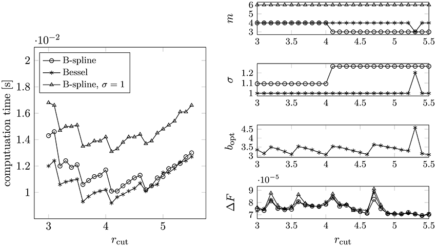
Figure 9. Measured runtimes for different values of r_cut (left). The required rms force accuracy was set to ε = 10⁻⁴. The parameters (right) were chosen by applying Algorithms 3.1, 4.1, and 4.2. For each r_cut we considered different combinations of m and σ, where we chose the one yielding the smallest computation time. Test case: N = 300 randomly distributed particles, box size: 10 × 10 × 10.

In contrast, in the case ε = 10⁻⁴ we obtain the following parameter combination.

• B-Spline: m = 4, σ ≈ 1.1 or m = 3, σ ≈ 1.25,

• Bessel: m = 4, σ = 1, b ≈ 3.3.

The same parameters are supposed to be optimal also for larger particle systems having the same particle/charge density, here $\frac{N}{V}=\frac{Q}{V}=0.3$, see Example 4.12. We expect fundamentally different optimal parameters when changing the particle density significantly.                                                                                                                                                                                                                                 □

4.3.3. Scale Parameters to Larger Particle Systems

As described above, all parameters can be tuned for a small particle system in order to apply the obtained set of parameters also to larger systems. Provided that Equation (29) is fulfilled, the rms errors are supposed to be of a comparable size among a set of systems having the same particle and charge density.

Example 4.12. We compute for each near field cutoff r_cut the Ewald parameters (α, β) as well as possible parameter combinations for the NFFT (support parameter m, oversampling factor σ) based on the small particle system considered in the last examples. The optimal set of parameters with respect to runtime is found by comparing the obtained runtimes for the large particle system.

We consider the following systems:

(i) N = 153600 randomly distributed particles in a cubic box with edge length L₁ = L₂ = L₃ = 80.

(ii) A so called cloud wall system containing N = 100800 particles in a non cubic box with edge length vector L = (60, 70, 80). The cloud wall system consists of two oppositely charged particle walls surrounded by further particles, which are randomly distributed. Such systems have been proposed in Arnold et al. [11] because of their significant long range part.

The measured optimal runtimes are plotted on the left hand side in Figures 10, 11. The corresponding NFFT parameters as well as the achieved rms force errors can be found on the right hand side, respectively.

FIGURE 10

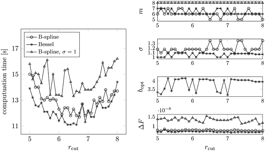
Figure 10. Measured runtimes for different values of r_cut (left). The required rms force accuracy was set to ε = 10⁻⁸. The parameters (right) were chosen by applying Algorithms 3.1, 4.1, and 4.2, setting N = 300 and L = (10, 10, 10) (see Example 4.11). For each r_cut we considered different combinations of m and σ, where we chose the one yielding the smallest computation time. Test case: N = 153600 randomly distributed particles, box size: 80 × 80 × 80.

FIGURE 11

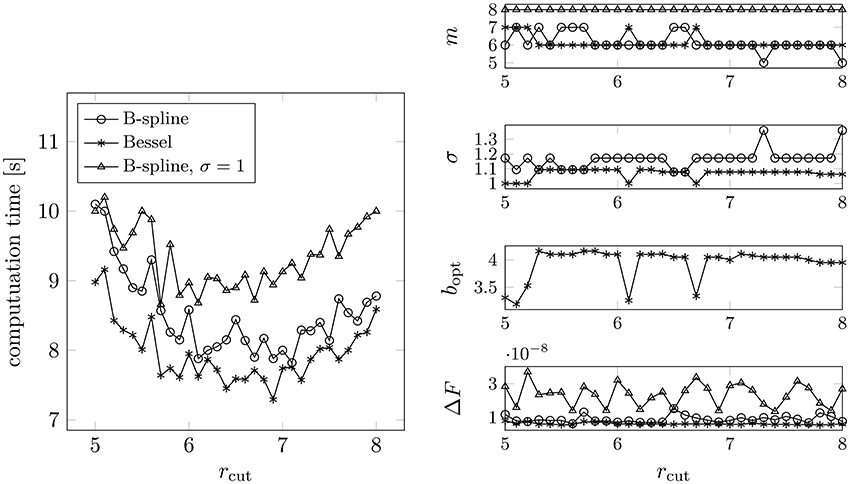
Figure 11. Measured runtimes for different values of r_cut (left). The required rms force accuracy was set to ε := 10⁻⁸. The parameters (right) were chosen by applying Algorithms 3.1, 4.1 and 4.2, setting N = 300 and L = (10, 10, 10) (see Example 4.11). For each r_cut we considered different combinations of m and σ, where we chose the one yielding the smallest computation time. Test case: cloud wall system, N = 100800 particles, box size: 60 × 70 × 80.

We can see that the optimal combinations of the NFFT parameters (m and σ) differ only slightly among the different particle systems. In contrast, the optimal near field cutoff changes with varying numbers of particles N, which is due to the fact that the near field computation scales like ${O}$(N), whereas ${O}$(N log N) arithmetic operations are needed for the far field.

In most cases it is more favorable in terms of computational costs to spend some oversampling in combination with a smaller supported window function. As in Example 4.11 we save approximately fifteen percent of runtime when applying the Bessel window function with oversampling instead of using the B-spline without oversampling. In the latter case we obtain even larger rms force errors.                                                                                                                                        □

Example 4.12 clearly shows that the parameters, which have been tuned for a small particle system, can be applied also to larger systems in order to keep the achieved accuracy among systems having the same charge as well as particle density almost constant. An optimization with respect to runtime is possible by measuring the required runtimes for different near field cutoffs r_cut. Thereby, we obtain unexpectedly large computation times in the case that the applied FFT mesh size shows an unprofitable factorization into prime factors, which makes it somewhat more difficult to predict the performance for larger particle systems, for which the FFT mesh size is appropriately scaled.

Note that for some fixed r_cut the computational cost required for the near field scales like ${O}$(N), assumed that the particles are homogeneously distributed. In contrast, the far field computations require ${O}$(N log N) arithmetical operations, i.e., for growing system size we expect that the optimal value for the near field cutoff r_cut is increasing, too. Thus, the tuning with respect to runtime should be done based on the original system instead of considering a smaller one.

In addition, we have seen that the possibility to use oversampling makes the P²NFFT method somewhat more flexible. In many cases a small oversampling factor is required in order to reach the requested accuracy. Moreover, we can reduce the computational costs since a window function of a smaller support can be used.

5. Conclusion

In the present work we studied the error behavior of the P²NFFT method, which is publicly available as a part of the ScaFaCoS library [19]. We investigated the performance of the algorithm for different window functions, namely B-splines, the Bessel I₀ function as well as the Gaussian, and presented an approach to predict the occurrent rms errors in the forces precisely and efficiently. Based on this, we also suggest a method to tune all involved parameters automatically.

Given a required accuracy and an appropriate near field cutoff r_cut, the splitting parameter α and the far field cutoff M can be computed easily by inverting the error formulas for the Ewald sums. In addition we can tune the NFFT parameters, as for instance the required oversampling factor and window specific parameters, in order to force the NFFT based approximation errors to be smaller than a given accuracy. For the efficient evaluation of the predicted errors we use an approximation of the function 1/x by a short sum of exponential terms, which enables a separation of the three dimensions. The presented numerical examples show that the error estimates are indeed very accurate and that the method can be tuned to a high precision via the proposed parameter tuning. In our examples we considered especially random particle systems, since the error estimates are obtained under the assumption that the particles are homogeneously distributed and that the different contributions to the overall error are uncorrelated. In the case that the Bessel or the Gaussian window function is used, the accuracy of the method very much depends on the window's shape parameter. We could improve the performance of the method significantly by tuning the shape parameter appropriately.

The results of the comparison between the different window functions can be summarized as follows. The applied combination of the near field cutoff r_cut, the splitting parameter α and the far field cutoff M very much influences which window function performs best in terms of accuracy. In general, we obtain the smallest approximation errors when using the Bessel or the B-spline window. In order to achieve a required precision, different combinations of all involved parameters are possible. It will especially depend on the used hardware and software which set of parameters is optimal with respect to runtime. All involved parameters can be tuned for a small particle system in order to apply the same parameters also to larger systems having the same particle density. We tested the described approach by considering sets of particle systems of increasing size. By applying the tuned parameters, we could achieve almost the same rms errors among systems having the same charge as well as particle density. The Bessel window function is in many cases the better choice with respect to the required computation time, since a smaller oversampling factor is needed. Thereby, an appropriate choice of the shape parameter is essential.

The analysis of the present approximation errors shows that the P²NFFT and the classical P³M method are in principle equivalent, if the B-spline window function without oversampling is used within the NFFT. The differences in the applied deconvolution schemes in terms of accuracy are negligible, especially if a high precision is required. The tests also show that spending some oversampling combined with a smaller support of the window function is in many cases more efficient than applying no oversampling, which requires the usage of a wider supported window function in order to achieve the same accuracy. The error analysis for the B-spline window shows that in certain cases the usage of oversampling is indeed necessary in order to reach a certain precision.

Author Contributions

The author confirms being the sole contributor of this work and approved it for publication.

Conflict of Interest Statement

The author declares that the research was conducted in the absence of any commercial or financial relationships that could be construed as a potential conflict of interest.

Acknowledgments

The author gratefully acknowledges support by the German Research Foundation (DFG), project PO 711/12-1, and thanks M. Pippig for customizing the P²NFFT software for the variation of the shape parameter. Moreover, the author would like to thank the reviewers for providing valuable suggestions. The publication costs of this article were funded by the DFG and the Technische Universität Chemnitz in the funding programme Open Access Publishing (ZY 112/1-4).

Supplementary Material

The Supplementary Material for this article can be found online at: https://www.frontiersin.org/article/10.3389/fphy.2016.00028

References

1. Hockney RW, Eastwood JW. Computer Simulation Using Particles. Bristol, PA: Taylor & Francis, Inc. (1988).

Google Scholar

2. Darden T, York D, Pedersen L. Particle mesh Ewald: an nlog(n) method for Ewald sums in large systems. J Chem Phys. (1993) 98:10089–92.

Google Scholar

3. Essmann U, Perera L, Berkowitz ML, Darden T, Lee H, Pedersen LG. A smooth particle mesh Ewald method. J Chem Phys. (1995) 103:8577–93.

PubMed Abstract | Google Scholar

4. Deserno M, Holm C. How to mesh up Ewald sums. I. A theoretical and numerical comparison of various particle mesh routines. J Chem Phys. (1998) 109:7678–93.

Google Scholar

5. Lindbo D, Tornberg AK. Spectral accuracy in fast Ewald-based methods for particle simulations. J Comput Phys. (2011) 230:8744–61. doi: 10.1016/j.jcp.2011.08.022

CrossRef Full Text | Google Scholar

6. Ewald PP. Die Berechnung optischer und elektrostatischer Gitterpotentiale. Ann Phys. (1921) 369:253–87.

PubMed Abstract | Google Scholar

7. Pippig M, Potts D. Particle simulation based on nonequispaced fast Fourier transforms. In: Sutmann G, Gibbon P, Lippert T, editors. Fast Methods for Long-Range Interactions in Complex Systems. Vol. 6, IAS-Series. Jülich: Forschungszentrum Jülich GmbH (2011). pp. 131–58.

8. PippigM, Potts D. Parallel three-dimensional nonequispaced fast Fourier transforms and their application to particle simulation. SIAM J Sci Comput. (2013) 35:C411–37. doi: 10.1137/120888478

CrossRef Full Text | Google Scholar

9. Hedman F, Laaksonen A. Ewald summation based on nonuniform fast Fourier transform. Chem Phys Lett. (2006) 425:142–7. doi: 10.1016/j.cplett.2006.04.106

CrossRef Full Text | Google Scholar

10. Fourmont K. Non equispaced fast Fourier transforms with applications to tomography. J Fourier Anal Appl. (2003) 9:431–50. doi: 10.1007/s00041-003-0021-1

CrossRef Full Text | Google Scholar

11. Arnold A, Fahrenberger F, Holm C, Lenz O, Bolten M, Dachsel H, et al. Comparison of scalable fast methods for long-range interactions. Phys Rev E (2013) 88:063308. doi: 10.1103/PhysRevE.88.063308

PubMed Abstract | CrossRef Full Text | Google Scholar

12. Nestler F, Pippig M, Potts D. Fast Ewald summation based on NFFT with mixed periodicity. J Comput Phys. (2015) 285:280–315. doi: 10.1016/j.jcp.2014.12.052

CrossRef Full Text | Google Scholar

13. Nestler F, Pippig M, Potts D. NFFT based fast Ewald summation for various types of periodic boundary conditions. In: Sutmann G, Grotendorst J, Gompper G, Marx D, editors. Computational Trends in Solvation and Transport in Liquids Vol. 28, IAS-Series. Jülich: Forschungszentrum Jülich GmbH (2015). pp. 575–98.

14. Greengard L, Rokhlin V. A fast algorithm for particle simulations. J Comput Phys. (1987) 73:325–48.

PubMed Abstract | Google Scholar

15. Dachsel H. An error-controlled Fast Multipole Method. J Chem Phys. (2010) 132:119901. doi: 10.1063/1.3358272

PubMed Abstract | CrossRef Full Text | Google Scholar

16. Kabadshow I, Dachsel H. The error-controlled Fast Multipole Method for open and periodic boundary conditions. In: Sutmann G, Gibbon P, Lippert T, editors. Fast Methods for Long-Range Interactions in Complex Systems, IAS-Series. Jülich: Forschungszentrum Jülich (2011). pp. 85–113.

17. Kabadshow I. Periodic Boundary Conditions and the Error-Controlled Fast Multipole Method. PhD thesis, Bergische Universität Wuppertal, Jülich (2012).

18. Kudin KN, Scuseria GE. Revisiting infinite lattice sums with the periodic Fast Multipole Method. J Chem Phys. (2004) 121:2886–90. doi: 10.1063/1.1771634

PubMed Abstract | CrossRef Full Text | Google Scholar

19. Arnold A, Bolten M, Dachsel H, Fahrenberger F, Gähler F, Halver R, et al. ScaFaCoS - Scalable Fast Coloumb Solvers. Available online at: http://www.scafacos.de

20. Pippig M. Massively Parallel, Fast Fourier Transforms and Particle-Mesh Methods. dissertation. Universitätsverlag Chemnitz (2015).

21. Dutt A, Rokhlin V. Fast Fourier transforms for nonequispaced data. SIAM J Sci Stat Comput. (1993) 14:1368–93.

PubMed Abstract | Google Scholar

22. Beylkin G. On the fast Fourier transform of functions with singularities. Appl Comput Harmon Anal. (1995) 2:363–81.

PubMed Abstract | Google Scholar

23. Steidl G. A note on fast Fourier transforms for nonequispaced grids. Adv Comput Math. (1998) 9:337–53.

Google Scholar

24. Ware AF. Fast approximate Fourier transforms for irregularly spaced data. SIAM Rev. (1998) 40:838–56.

Google Scholar

25. Potts D, Steidl G, Tasche M. Fast Fourier transforms for nonequispaced data: a tutorial. In: Benedetto JJ, Ferreira PJSG, editors. Modern Sampling Theory: Mathematics and Applications, Boston, MA: Birkhäuser (2001). pp. 247–70.

26. Greengard L, Lee JY. Accelerating the nonuniform fast Fourier transform. SIAM Rev. (2004) 46:443–54.

PubMed Abstract | Google Scholar

27. Keiner J, Kunis S, Potts D. Using NFFT3 - a software library for various nonequispaced fast Fourier transforms. ACM Trans Math Softw. (2009) 36:1–30. doi: 10.1145/1555386.1555388

CrossRef Full Text

28. Duijndam AJW, Schonewille MA. Nonuniform fast Fourier transform. Geophysics (1999) 64:539–51.

PubMed Abstract | Google Scholar

29. Jacob M. Optimized least-square nonuniform Fast Fourier Transform. IEEE Trans Signal Process. (2009) 57:2165–77.

PubMed Abstract | Google Scholar

30. Nestler F. Automated parameter tuning based on RMS errors for nonequispaced FFTs. Adv Comput Math. (2015). doi: 10.1007/s10444-015-9446-8

CrossRef Full Text | Google Scholar

31. Potts D, Steidl G. Fast summation at nonequispaced knots by NFFTs. SIAM J Sci Comput. (2003) 24:2013–37. doi: 10.1137/S1064827502400984

CrossRef Full Text | Google Scholar

32. Kaiser JF. Digital filters. In: Kuo FF, Kaiser JF, editors. System Analysis by Digital Computer. New York, NY: Wiley (1966).

PubMed Abstract

33. Jackson JI, Meyer CH, Nishimura DG, Macovski A. Selection of a convolution function for Fourier inversion using gridding. IEEE Trans Med Imaging (1991) 10:473–8.

PubMed Abstract | Google Scholar

34. Kolafa J, Perram JW. Cutoff errors in the Ewald summation formulae for point charge systems. Mol Simul. (1992) 9:351–68.

Google Scholar

35. de Leeuw SW, Perram JW, Smith ER. Simulation of electrostatic systems in periodic boundary conditions. I. Lattice sums and dielectric constants. Proc R Soc London Ser A (1980) 373:27–56.

Google Scholar

36. Ballenegger V. Communication: on the origin of the surface term in the Ewald formula. J Chem Phys. (2014) 140:16. doi: 10.1063/1.4872019

PubMed Abstract | CrossRef Full Text | Google Scholar

37. Frenkel D, Smit B. Understanding Molecular Simulation: From Algorithms to Applications. San Diego; San Francisco; New York: Academic Press (2002).

Google Scholar

38. Hummer G, Pratt LR, García AE. Free energy of ionic hydration. J Phys Chem. (1996) 100:1206–15.

PubMed Abstract | Google Scholar

39. Deserno M, Holm C. How to mesh up Ewald sums. II. An accurate error estimate for the Particle-Particle-Particle-Mesh algorithm. J Chem Phys. (1998) 109:7694–701.

40. Wang ZW, Holm C. Estimate of the cutoff errors in the Ewald summation for dipolar systems. J Chem Phys. (2001) 115:6277–798. doi: 10.1063/1.1398588

CrossRef Full Text | Google Scholar

41. Arnold A, de Joannis J, Holm C. Electrostatics in periodic slab geometries. II. J Chem Phys. (2002) 117:2503. doi: 10.1063/1.1491954

CrossRef Full Text | Google Scholar

42. Pippig M. PFFT - An extension of FFTW to massively parallel architectures. SIAM J Sci Comput. (2013) 35:C213–36. doi: 10.1137/120885887

CrossRef Full Text | Google Scholar

43. Wang YL, Hedman F, Porcu M, Mocci F, Laaksonen A. Non-uniform FFT and its applications in particle simulations. Appl Math. (2014) 5:520–541. doi: 10.4236/am.2014.53051

CrossRef Full Text | Google Scholar

44. Neelov A, Holm C. Interlaced P3M algorithm with analytical and ik-differentiation. J Chem Phys. (2010) 132:234103. doi: 10.1063/1.3430521

PubMed Abstract | CrossRef Full Text | Google Scholar

45. Roy R, Kailath T. ESPRIT—estimation of signal parameters via rotational invariance techniques. IEEE Trans Acoust Speech Signal Process. (1989) 37:984–94.

PubMed Abstract | Google Scholar

46. Potts D, Tasche M. Parameter estimation for nonincreasing exponential sums by Prony-like methods. Linear Algebra Appl. (2013) 439:1024–39. doi: 10.1016/j.laa.2012.10.036

CrossRef Full Text | Google Scholar

47. Hackbusch W. Entwicklungen nach Exponentialsummen. Technical report, Max Planck Institute for Mathematics in the Sciences (2005). Available online at: http://www.mis.mpg.de/de/publications/andere-reihen/tr/report-0405.html

48. Ballenegger V, Cerdà JJ, Holm C. How to convert SPME to P3M: influence functions and error estimates. J Chem Theory Comput. (2012) 8:936–47. doi: 10.1021/ct2001792

PubMed Abstract | CrossRef Full Text | Google Scholar

49. Johnson S, Carvellino A, Wuttke J. Libcerf, Numeric Library for Complex Error Functions. Available online at: http://apps.jcns.fz-juelich.de/libcerf

50. Pippig M. PNFFT - Parallel Nonequispaced FFT Software Library. Available online at: https://github.com/mpip/pnfft