CVaR hedging under stochastic interest rate

1. Introduction

The problem of pricing and hedging of a contingent claim is well understood in the context of a complete market. Given a sufficient allocation of initial wealth, every contingent claim can be replicated by a self-financing trading strategy, thereby being hedged perfectly. The cost of replication defines the price of the claim, and can be computed as the expectation of the claim under a unique equivalent martingale measure. The cost of perfect hedging however, is often too high for investors in the financial market. Given a limited amount of capital, investors always seek as many business opportunities as possible while taking the total risk associated under control. As such, more and more studies focus on exploiting partial hedging techniques.

The main characteristic of partial hedging is that it allows investors to allocate a smaller amount of initial capital than in the case of perfect hedging, while still managing the risk in a systematic way. Explicitly, let L denote the loss which equals the difference between the payoff of a contingent claim and that of a replicating portfolio, partial hedging aims to minimize the risk of the loss L. The performance of partial hedging mostly relies on the selection of the underlying risk measure. Different partial hedging approaches have been proposed and examined in the literature. The well-known examples are quadratic hedging and quantile hedging. Quadratic hedging minimizes the expectation of a quadratic error (L²). Such a measure has been criticized for the consequence of penalizing both loss and profit equally, also for not being able to capture the heavy-tailness phenomena in the financial market. Quantile hedging is probably the most studied approach. The first papers appearing in this research area were [1], [2] and [3]. Later [4], [5] and [6] applied the quantile hedging technique on pricing equity-linked life insurance products. Quantile hedging maximizes the probability that a hedge is successful by applying a dynamic version of the static Varlue-at-Risk (VaR). VaR has been adopted as a standard risk measure in the financial industry. It has a number of deficiencies recognized by financial professionals. More recently, [7] suggested addressing partial hedging problem by employing conditional Varlue-at-Risk (CVaR). CVaR is a risk measure that is a superior alternative to VaR in that it conveys information about the average loss exceeds the VaR level and also satisfies the sub-additive property.

In this paper we follow [7] adopting CVaR as the risk quantifier. However, rather than assuming a constant interest rate, we apply Heath-Jarrow-Morton (HJM) methodology proposed by Heath et al. [8] to model the stochastic process of interest rate. HJM is widely accepted as the most general framework derived by directly modeling the dynamics of instantaneous forward-rates. It is well known that in a no-arbitrage world there exists an explicit relationship between the drift and volatility of the forward-rate dynamics, thus forward price valuing can be done from the knowledge of the volatility process and the initial rate. Much of the existing literature pays attention to the application of stochastic interest rate models, for example, Ciurlia and Gheno [9] and Jalen and Mamon [10]. Gao et al. [11] studies quantile hedging of life insurance contracts with stochastic interest rate setting. However, the subject of CVaR hedging in a stochastic interest rate environment has not been studied.

Our main objective is to construct a partial hedging strategy by using CVaR. We take up two issues: given the initial capital constraint we minimize the CVaR of the loss L; by prescribing a bound on the risk, we minimize the cost of the target portfolio. As an illustration of this hedging technique we derive hedging strategies for a European call option. Hedging of options is one of the basic problems in modern mathematical finance in the theory and in the applications. This problem was initiated in classical works of Black and Scholes [12] and Merton [13], since that time a number of works were devoted to different aspects of the problem. In this paper we consider a European call option with the Black Scholes setting under HJM framework; explicit formulas are derived. We also investigate CVaR hedging problems by using the real financial data.

An outline of this paper is as follows: Section 2 reviews CVaR and CVaR minimization problems, and then derives the solutions to the minimization problems for a non-discounted portfolio; Section 3 illustrates HJM methodology, and tackles CVaR hedging problem under HJM framework. The last subsection of Section 3 demonstrates the explicit solutions of the hedging problems by taking a european call option as a motivating example; Section 4 gives a numerical example of how CVaR hedging techniques can be applied on a call option, where overnight ICE LIBOR rate for US dollars and S&P 500 index price are employed.

2. Problem Setup and Main Results

2.1. Conditional Value-at-Risk

The partial hedging problem considers controlling the risk of portfolio loss under certain constrains. The performance of partial hedging mostly relies on the selection of the underlying risk measure. The most studied approach in the literature, quantile hedging, maximizes the probability that a hedge is successful by applying a dynamic version of the static Varlue-at-Risk (VaR). VaR has been widely adopted as a standard risk measure in the financial industry. However, It has been criticized for it's not being subadditive, meaning that it cannot account for diversification. The conditional value-at-risk CVaR which is closely related to VaR, is often considered to be a better alternative. Unlike VaR, CVaR is a coherent risk measure, thus subadditive. CVaR focuses on the entire tail of the loss distribution, which makes it greater than VaR.

To define CVaR, let (Ω, {_t}_{t∈[0, T]}, , ℙ) be a standard probability space and L be a -measurable random variable characterizing the loss. We assume that E^ℙ[L] < ∞.

The VaR of the loss L at a confidence level ϵ ∈ (0, 1) is defined as:

$Va{R}_{ϵ}(L)=\inf \{x:\mathbb{P}(L>x)\le 1-ϵ\},$

and CVaR at a confidence level ϵ ∈ (0, 1) is defined as:

$\begin{array}{l}CVa{R}_{ϵ}(L)=\frac{1}{1-ϵ}[E^{\mathbb{P}}[L{1}_{\{L\ge Va{R}_{ϵ}(L)\}}]+\\ Va{R}_{ϵ}(L)(1-ϵ-\mathbb{P}(L\ge Va{R}_{ϵ}(L)))].\end{array}$

If the cumulative distribution function F_L(l): = ℙ(L ≤ l) is continuous, VaR is simply the inverse function of F_L, and CVaR can be rewritten as:

$CVa{R}_{ϵ}(L)=E^{\mathbb{P}}[L|L\ge Va{R}_{ϵ}(L)],$

which equals to the expected shortfall (ES), and

$CVa{R}_{ϵ}(L)=\frac{1}{1-ϵ}{\displaystyle {\int }_{ϵ}^{1}V}a{R}_u(L)du,$

which equals to the average value-at-risk (AVaR).

There are convenient methods of computing and estimating CVaR. Rockafellar and Uryasev [14] showed the possibility of computing both VaR and CVaR simultaneously by introducing an auxiliary function:

$F_{ϵ}(z)=z+\frac{1}{1-ϵ}{E}^{\mathbb{P}}[{(L-z)}^{+}].$

CVaR of the loss L is the solution of the minimization problem:

$\begin{array}{ll}CVa{R}_{ϵ}(L)=\underset{z\in ℝ}{\min }{F}_{ϵ}(x,z)\hfill & (1)\hfill \end{array}$

2.2. Problem Setup

Consider a portfolio consists of a risky asset S and a default-free bond R. Let {S(t)}_{t∈[0, T]} represents the price of the asset S at time index t, and {R(t)}_{t∈[0, T]} represents the price of the bond R at time t. We assume that both S(t) and R(t) are _t measurable. Define ξ_S(t) and ξ_R(t) as the number of shares held on S and R at time t∈[0, T]. The value of the portfolio V at time t is give by:

$V(t)={\xi }_S(t)S(t)+{\xi }_R(t)R(t),t\in [0,T].$

Let ξ(t): = (ξ_S(t),ξ_B(t)) be a self-financing strategy, then V(t) satisfies the following stochastic differential equation:

$V(t)=V(0)+{\displaystyle {\int }_0^t{\xi }_S}(s)dS(s)+{\displaystyle {\int }_0^t{\xi }_R}(s)dR(s),t\in [0,T].$

A strategy {ξ_t}_{t∈[0, T]} is admissible if

$V(t)\ge 0\text{, for all }t\in [0,T]\text{, }\mathbb{P}-a.s.$

In the context of a complete market, every contingent claim can be replicated by a self-financing strategy {ξ*(t)}_{t∈[0, T]}. Let H(T), (H(T) ≥ 0), be the payoff of a contingent claim at time T; H(T) is a _T measurable random variable. The cost of the replication defines the price of the contingent claim: let ℚ be the unique equivalent martingale measure, the value of the claim can be replicated by {ξ*(t)}_{t∈[0, T]} which requires an initial amount of

$V^{\ast }(0)={\xi }_S^{\ast }(0)S(0)+{\xi }_B^{\ast }(0)B(0)=E^{\mathbb{Q}}[R{(T)}^{-1}H(T)].$

Such a strategy is served as a perfect hedge for the claim H(T). In the case of partial hedging it only requires a smaller initial amount V(0) of no larger than ν, that is,

$V(0)\le \nu <E^{\mathbb{Q}}[R{(T)}^{-1}H(T)].$

What would be the optimal partial hedge that can be achieved?

An investor who shorts the contingent claim H(T) wants to construct a portfolio {V(t)}_{t∈[0, T]} with a purpose of hedging the potential loss L = H(T) − V(T) at maturity time T. Note that in a complete market if the initial value V(0) is smaller than the price of the claim, then L ≠ 0. Our goal is to find the most efficient strategy such that the risk is controlled. This paper takes two issues in locating optimal strategy: one is to minimize the CVaR of the loss L, with respect to the constraint that the initial cost V(0) is smaller than some number ν:

$\begin{array}{ll}\begin{array}{l}\underset{V(0),\xi }{\min }CVa{R}_{ϵ}(H(T)-V(T))\hfill \\ \text{ s}.\text{t}.V(0)\le \nu \hfill \end{array}\hfill & (2)\hfill \end{array}$

where ν < E^ℚ[R(T)⁻¹ H(T)]; the other one is to minimize the hedging cost V(0) so that the CVaR is less than or equal to a number c:

$\begin{array}{ll}\begin{array}{l}\underset{V(0),\xi }{\min }V(0)=E^{\mathbb{Q}}[R{(T)}^{-1}V(T)]\\ \text{ s}.\text{t}.CVa{R}_{ϵ}(H(T)-V(T))\le c\end{array}\hfill & (3)\hfill \end{array}$

These two problems are discussed in the following sections.

2.3. Minimizing CVaR

We first consider the CVaR minimizing problem Equation (2). According to the CVaR representation Equation (1) we have

$\begin{array}{l}{\min }_{V(0),\xi }{\min }_{z\in ℝ}z+\frac{1}{1-ϵ}{E}^{\mathbb{P}}[{(H(T)-V(T)-z)}^{+}]\\ \text{ s}.\text{t}.V(0)\le \nu \end{array}$

Melnikov and Smirnov [7] shows that we can interchange the order of two minimization problems:

$\begin{array}{ll}\begin{array}{l}{\min }_{z\in ℝ}z+\frac{1}{1-ϵ}{\min }_{V(0),\xi }{E}^{\mathbb{P}}[{(H(T)-V(T)-z)}^{+}]\\ \text{ s}.\text{t}.V(0)\le \nu \end{array}\hfill & (4)\hfill \end{array}$

For z ≥ 0, we have (H(T) − V(T) − z)⁺ = ((H(T) − z)⁺ − V(T))⁺; then we can write Equation (4) to be

$\begin{array}{ll}\begin{array}{l}{\min }_{V(0),\xi }{E}^{\mathbb{P}}[{({(H(T)-z)}^{+}-V(T))}^{+}]\\ \text{ s}.\text{t}.V(0)\le \nu \end{array}\hfill & (5)\hfill \end{array}$

In this paper, we quantify the loss of an undiscounted portfolio. This is different from Föllmer and Leukert [1], Gao et al. [11] and Melnikov and Smirnov [7]. Despite the fact that we want to control the risk of a hedging portfolio at maturity T rather than its current value, dealing with CVaR of a discounted portfolio would result in computational inefficiency. To see this, take a call option H(T) = (S(T) − K)⁺ as an example, which we will see later: by taking the discount factor into account, (H(T) − z)⁺ in Equation (5) is replaced by (R(T)⁻¹H(T) − z)⁺ = R(T)⁻¹(H(T) − zR(T))⁺ = R(T)⁻¹(S(T) − K − zR(T))⁺, where S(T) − zR(T) is a linear combination of two log normal random variables, and difficult to generate a closed solution.

To solve the optimization problem in Equation (5), we suggest applying the measure transformation method to the discounted problem before addressing the undiscounted one. The discounted problem was well-studied by Föllmer and Leukert [2]:

Theorem 1. Let H(T) be the payoff of a contingent claim, then the optimal hedging strategy (V*(0),ξ*) of the shortfall minimization problem:

$\begin{array}{l}{\min }_{V(0),\xi }{E}^{\mathbb{P}}[R{(T)}^{-1}{(H(T)-V(T))}^{+}]\\ s.t.V(0)\le \nu <E^{\mathbb{Q}}[R{(T)}^{-1}H(T)]\end{array}$

is the perfect hedge for the claim H*(T) = H(T)ψ*, where

$\begin{array}{l}{\psi }^{*}=1_{\{\frac{d\mathbb{P}}{d\mathbb{Q}}>a^{*}\}}+\gamma 1_{\{\frac{d\mathbb{P}}{d\mathbb{Q}}=a^{*}\}}\hfill \\ a^{*}=\inf \{a\ge 0:E^{\mathbb{Q}}[R{(T)}^{-1}H(T)1_{\{\frac{d\mathbb{P}}{d\mathbb{Q}}>a\}}]\le \nu \}\hfill \\ \gamma =\frac{\nu -E^{\mathbb{Q}}[R{(T)}^{-1}H(T)1_{\{\frac{d\mathbb{P}}{d\mathbb{Q}}>a^{*}\}}]}{E^{\mathbb{Q}}[R{(T)}^{-1}H(T)1_{\{\frac{d\mathbb{P}}{d\mathbb{Q}}=a^{*}\}}]}\hfill \end{array}$

By Theorem 1, we can generate the following theorem for the undiscounted process:

Theorem 2. Let H(T) be the payoff of a contingent claim, then the optimal hedging strategy (V*(0), ξ*) of the shortfall minimization problem:

$\begin{array}{l}{\min }_{V(0),\xi }{E}^{\mathbb{P}}[{(H(T)-V(T))}^{+}]\\ s.t.V(0)\le \nu <E^{\mathbb{Q}}[R{(T)}^{-1}H(T)]\end{array}$

is the perfect hedge for the claim H*(T) = H(T)ψ*, where

$\begin{array}{l}{\psi }^{*}=1_{\{R(T)\frac{d\mathbb{P}}{d\mathbb{Q}}>a^{*}\}}+\gamma 1_{\{R(T)\frac{d\mathbb{P}}{d\mathbb{Q}}=a^{*}\}}\\ a^{*}=\inf \{a\ge 0:E^{\mathbb{Q}}[R{(T)}^{-1}H(T)1_{\{R(T)\frac{d\mathbb{P}}{d\mathbb{Q}}>a\}}]\le \nu \}\\ \gamma =\frac{\nu -E^{\mathbb{Q}}[R{(T)}^{-1}H(T)1_{\{R(T)\frac{d\mathbb{P}}{d\mathbb{Q}}>a^{*}\}}]}{E^{\mathbb{Q}}[R{(T)}^{-1}H(T)1_{\{R(T)\frac{d\mathbb{P}}{d\mathbb{Q}}=a^{*}\}}]}\end{array}$

Proof. Define

$\frac{d{\mathbb{P}}^{\ast }}{d\mathbb{P}}=\frac{R(T)}{E^{\mathbb{P}}[R(T)]},$

then

$\begin{array}{ll}\begin{array}{l}{E}^{\mathbb{P}}[{(H(T)-V(T))}^{+}]=E[R(T)]E^{{\mathbb{P}}^{\ast }}[R{(T)}^{-1}\\ {(H(T)-V(T))}^{+}].\end{array}\hfill & (6)\hfill \end{array}$

To minimize Equation (6) we apply Theorem 1, then

$\frac{d{\mathbb{P}}^{\ast }}{d\mathbb{Q}}=\frac{R(T)}{E^{\mathbb{P}}[R(T)]}\frac{d\mathbb{P}}{d\mathbb{Q}},$

finishes the proof.□

We can apply Theorem 2 to solve problem Equation (5) by letting $\tilde{H}$(T): = (H(T) − z)⁺; and that gives the solution to Equation (2). Based on the result in Melnikov and Smirnov [7], we conclude that:

Theorem 3. The optimal strategy (V(0)*,ξ*) for the CVaR minimization problem Equation (2) is a perfect hedge for the contingent claim (H − z*)⁺ψ*(z*), where ψ*(z) is given by

$\begin{array}{l}{\psi }^{*}(z)=1_{\{R(T)\frac{d\mathbb{P}}{d\mathbb{Q}}>a^{*}(z)\}}+\gamma (z)1_{\{R(T)\frac{d\mathbb{P}}{d\mathbb{Q}}=a^{*}(z)\}}\\ a^{*}(z)=\inf \{a\ge 0:E^{\mathbb{Q}}[R{(T)}^{-1}{(H(T)-z)}^{+}{1}_{\{R(T)\frac{d\mathbb{P}}{d\mathbb{Q}}>a\}}]\le \nu \}\\ \gamma (z)=\frac{\nu -E^{\mathbb{Q}}[R{(T)}^{-1}{(H(T)-z)}^{+}{1}_{\{R(T)\frac{d\mathbb{P}}{d\mathbb{Q}}>a^{*}(z)\}}]}{E^{\mathbb{Q}}[R{(T)}^{-1}{(H(T)-z)}^{+}{1}_{\{R(T)\frac{d\mathbb{P}}{d\mathbb{Q}}=a^{*}(z)\}}]}\end{array}$

and z* is the solution of minimization problem:

$\underset{z>0}{\min }c(z)\text{}=\text{}\{\begin{array}{ll}z\text{}+\text{}\frac{1}{1-ϵ}{E}^{\mathbb{P}}[{(H(T)-z)}^{+}(1-{\psi }^{\ast }(z))]\hfill & \text{}if0\le z<\widehat{z}\hfill \\ z\hfill & ifz\ge \widehat{z}\hfill \end{array}$

ẑ is the solution of

$E^{\mathbb{Q}}[R{(T)}^{-1}{(H(T)-z)}^{+}]=\nu$

Note that only when z ≥ 0 can we use the result of Equation (5) to solve Equation (2). Nonethless, we do not need to worry about the case when z < 0 because we assume that for any ϵ that is close enough to 1, the optimal ẑ that equals to the VaR_ϵ of the portfolio is always nonnegative.

2.4. Minimizing Hedging Costs

In this subsection we address the hedging costs minimization problem arised in Equation (3). Let us take the shortfall optimization problem as the point of departure.

Theorem 4. Let H(T) be the payoff of a contingent claim, then the optimal hedging strategy (V*(0),ξ*) of the shortfall minimization problem:

$\begin{array}{ll}\begin{array}{l}{\min }_{V(0),\xi }V(0)=E^{\mathbb{Q}}[R{(T)}^{-1}V(T)]\\ s.t.E^{\mathbb{P}}[{(H(T)-V(T))}^{+}]\le c<E^{\mathbb{P}}[H(T)]\end{array}\hfill & (7)\hfill \end{array}$

is the perfect hedge for the claim H*(T) = H(T)(1−ψ*), where

$\begin{array}{l}{\psi }^{\ast }=1_{\{R{(T)}^{-1}\frac{d\mathbb{Q}}{d\mathbb{P}}>a^{\ast }\}}+\gamma 1_{\{R{(T)}^{-1}\frac{d\mathbb{Q}}{d\mathbb{P}}=a^{\ast }\}}\\ a^{\ast }=\inf \{a\ge 0:E^{\mathbb{P}}[H(T)1_{\{R{(T)}^{-1}\frac{d\mathbb{Q}}{d\mathbb{P}}>a\}}]\le c\}\\ \gamma =\frac{c-E^{\mathbb{P}}[H(T)1_{\{R{(T)}^{-1}\frac{d\mathbb{Q}}{d\mathbb{P}}>a^{\ast }\}}]}{E^{\mathbb{P}}[H(T)1_{\{R{(T)}^{-1}\frac{d\mathbb{Q}}{d\mathbb{P}}=a^{\ast }\}}]}\end{array}$

Proof. Follow the proof of Theorem 3, we reformulate the problem Equation (7) to be:

$\begin{array}{ll}\begin{array}{l}{\min }_{V(0),\xi }V(0)=E^{\mathbb{Q}}[R{(T)}^{-1}V(T)]\\ \text{s}.\text{t}.E^{{\mathbb{P}}^{\ast }}[R{(T)}^{-1}{(H(T)-V(T))}^{+}]\le \frac{c}{E^{\mathbb{P}}[R(T)]}\end{array}\hfill & (8)\hfill \end{array}$

where

$\frac{d{\mathbb{P}}^{\ast }}{d\mathbb{P}}=\frac{R(T)}{E^{\mathbb{P}}[R(T)]}$

As in Föllmer and Leukert [1] and Föllmer et al. [15], we rewrite the problem Equation (8) by employing a random test ψ:

To see this, first we assume that $\widehat{V}$(T) is the solution of problem Equation (8) and $\tilde{\psi }$ is the solution of problem Equation (9), then $\tilde{V}$(T): = H(T)(1 − $\tilde{\psi }$) satisfies the constraint within Equation (8). Thus, we have

$\begin{array}{l}{E}^{\mathbb{Q}}[R{(T)}^{-1}H(T)(1-\tilde{\psi })]=E^{\mathbb{Q}}[R{(T)}^{-1}\tilde{V}(T)]\ge \\ E^{\mathbb{Q}}[R{(T)}^{-1}\widehat{V}(T)].\end{array}$

On the other side $\widehat{\psi }$: = (1 − $\widehat{V}$(T)/H(T))1_{{$\widehat{V}$(T)≤H(T)}} ∈ [0,1] satisfies the constraint within Equation (9), and

$\begin{array}{l}{E}^{\mathbb{Q}}[R{(T)}^{-1}H(T)(1-\tilde{\psi })]\le E^{\mathbb{Q}}[R{(T)}^{-1}H(T)(1-\widehat{\psi })]\le \\ E^{\mathbb{Q}}[R{(T)}^{-1}\widehat{V}(T)].\end{array}$

Apply Neyman-Pearson's lemma we can solve problem Equation (9). See [15] for details. The solution is given by ψ*.□

By following lemma 2.5 and lemma 2.6 in Melnikov and Smirnov [7] we have

Theorem 5. If E^ℙ[H] > c(1 − ϵ) and E^ℙ[(H − c)⁺] > 0, then the optimal strategy (V(0)*,ξ*) for the hedging costs minimization problem Equation (3) is a perfect hedge for the contingent claim (H − z*)⁺(1 − ψ*(z*)), where ψ*(z) is given by

$\begin{array}{l}{\psi }^{\ast }(z)=1_{\{R{(T)}^{-1}\frac{d\mathbb{Q}}{d\mathbb{P}}>a^{\ast }(z)\}}+\gamma (z)1_{\{R{(T)}^{-1}\frac{d\mathbb{Q}}{d\mathbb{P}}=a^{\ast }(z)\}}\\ a^{\ast }(z)=\inf \{a\ge 0:E^{\mathbb{P}}[{(H(T)-z)}^{+}{1}_{\{R{(T)}^{-1}\frac{d\mathbb{Q}}{d\mathbb{P}}>a\}}]\\ \le (c-z)(1-ϵ)\}\\ \gamma (z)=\frac{(c-z)(1-ϵ)-E^{\mathbb{P}}[{(H(T)-z)}^{+}{1}_{\{R{(T)}^{-1}\frac{d\mathbb{Q}}{d\mathbb{P}}>a^{\ast }(z)\}}]}{E^{\mathbb{P}}[{(H(T)-z)}^{+}{1}_{\{R{(T)}^{-1}\frac{d\mathbb{Q}}{d\mathbb{P}}=a^{\ast }(z)\}}]}\end{array}$

and z* is the solution of

$\underset{{}_{z\in [0,c]}}{\min }{E}^{\mathbb{Q}}[R{(T)}^{-1}{(H-z)}^{+}(1-{\psi }^{\ast }(z))].$

3. CVaR Hedging for European Call Option Under HJM Framework

3.1. Option Pricing Under HJM

HJM is widely accepted as the most general framework derived by directly modeling the dynamics of instantaneous forward-rates. In this subsection we tackle the option pricing problem under HJM framework. Take a European call option as an example, the objective function for pricing the option is formulated as:

$V(0)=E^{\mathbb{Q}}[R{(T)}^{-1}{(S(T)-K)}^{+}],$

where T is the maturity and K is the strike price of the option. We start by introducing the basic assumptions concerning the financial setup.

The setup is similar to Amin and Jarrow [16] and Gao et al. [11]. Fix a complete probability space (Ω, {_t}_{t∈[0, T]},,ℙ) where ℙ is the real-world probability measure. Let {B^ℙ₁(t)}_{t∈[0, T]} be a standard Brownian motion defined on (Ω, {_t}_{t∈[0, T]},,ℙ). For a given continuous initial forward rate curve {f(0, t)}_{t∈[0, T]}, we assume that the forward rate process follows Itô's formula dynamics

$f(t,T)=f(0,T)+{\displaystyle {\int }_0^t\alpha }(u,T)du+{\displaystyle {\int }_0^t\sigma }(u,T)d{B}_1^{\mathbb{P}}(u),$

where α(t, T) and σ(t, T) are drift and volatility processes, respectively.

The spot interest rate at time t, {r(t)}_{t∈[0, T]} is given by the instantaneous forward rate of a forward contract, i.e.,

$r(t)=f(t,t)=f(0,t)+{\displaystyle {\int }_0^t\alpha }(u,t)du+{\displaystyle {\int }_0^t\sigma }(u,t)d{B}_1^{\mathbb{P}}(u).$

For every maturity time T, the forward price {P(t, T)}_{t∈[0, T]} can be written as

$\begin{array}{l}P(t,T)=\exp (\text{}-\text{}{\displaystyle {\int }_t^{T}f}(t,u)du)\\ =P(0,T)+{\displaystyle {\int }_0^{t}P}(u,T)\left(r(u)-{\alpha }^{\ast }(u,T)+\text{}\frac{1}{2}{\sigma }^{\ast }{(u,T)}^2\right)\\ du-{\displaystyle {\int }_0^{t}P}(u,T){\sigma }^{\ast }(u,T)d{B}_1^{\mathbb{P}}(u),\end{array}$

where

$\begin{array}{l}{\sigma }^{\ast }(t,T)={\displaystyle {\int }_t^T\sigma }(t,u)du,\\ {\alpha }^{\ast }(t,T)={\displaystyle {\int }_t^T\alpha }(t,u)du.\end{array}$

The dynamic of the price process {R(t)}_{t∈[0, T]} for a zero-coupon bond is described by

$\begin{array}{l}R(t)=\exp \left({\displaystyle {\int }_0^{t}r}(u)du\right)\\ =\frac{1}{P(0,t)}\exp \left({\displaystyle {\int }_0^t{\alpha }^{\ast }}(s,t)ds+{\displaystyle {\int }_0^t{\sigma }^{\ast }}(s,t)d{B}_1^{\mathbb{P}}(s)\right).\end{array}$

Consider the return process of the risky-asset S. Given the probability space (Ω, {_t}_{t∈[0, T]},,ℙ), where {_t}_{t∈[0, T]} is the augmented filtration driven by two independent Brownian motions {(B^ℙ₁(t), B^ℙ₂(t))}_{t∈[0, T]} initialized at zero. The dynamic of the asset price is governed by the stochastic differential equation:

$\begin{array}{l}S(t)=S(0)+{\displaystyle {\int }_0^t(\mu (u)+r(u))S(u)}du+{\displaystyle {\int }_0^t{\sigma }_1}(u)S(u)d{B}_1^{\mathbb{P}}(u)\\ +{\displaystyle {\int }_0^t{\sigma }_2}(u)S(u)d{B}_2^{\mathbb{P}}(u)\end{array}$

where {μ(t)}_{t∈[0, T]} denotes the excess return process without randomness. The summation of μ and r represents the expected growth rate.

Let ℚ be a probability measure which is equivalent to ℙ. The Radon-Nikodym derivative $\frac{d\mathbb{Q}}{d\mathbb{P}}$ transforms the real-world measure ℙ into the risk-neutral measure ℚ with the assumption of no-arbitrage, i.e.,

$\begin{array}{l}\frac{d\mathbb{Q}}{d\mathbb{P}}=\exp (-\frac{1}{2}{\displaystyle {\int }_0^T{\theta }_1}{(u)}^{2}du-\frac{1}{2}{\displaystyle {\int }_0^T{\theta }_2}{(u)}^{2}du\\ +{\displaystyle {\int }_0^T{\theta }_1}(u)d{B}_1^{\mathbb{P}}(u)+{\displaystyle {\int }_0^T{\theta }_2}(u)d{B}_2^{\mathbb{P}}(u)).\end{array}$

By Girsanov's theorem, the processes

$\begin{array}{ll}{B}_1^{\mathbb{Q}}(t)=B_1^{\mathbb{P}}(t)-{\displaystyle {\int }_0^t{\theta }_1}(u)du,\hfill & (10)\hfill \end{array}$

$\begin{array}{ll}{B}_2^{\mathbb{Q}}(t)=B_2^{\mathbb{P}}(t)-{\displaystyle {\int }_0^t{\theta }_2}(u)du,\hfill & (11)\hfill \end{array}$

are two independent ℚ-Brownian motions. As both {B(t)⁻¹S(t)}_{t∈[0, T]} and {B(t)⁻¹P(t, T)}_{t∈[0, T]} are martingales under ℚ, we have

$\begin{array}{l}-{\alpha }^{\ast }(t,T)+\frac{1}{2}{\sigma }^{\ast }{(t,T)}^2-{\sigma }^{\ast }(t,T){\theta }_1(t)=0,\\ \mu (t)+{\sigma }_1(t){\theta }_1(t)+{\sigma }_2(t){\theta }_2(t)=0.\end{array}$

Thus,

$\begin{array}{l}{\theta }_1(t)=\frac{-{\alpha }^{\ast }(t,T)+\frac{1}{2}{\sigma }^{\ast }{(t,T)}^2}{{\sigma }^{\ast }(t,T)},\\ {\theta }_2(t)=\frac{-\mu (t){\sigma }^{\ast }(t,T)+{\sigma }_1(t){\alpha }^{*}(t,T)-\frac{1}{2}{\sigma }_1(t){\sigma }^{\ast }{(t,T)}^2}{{\sigma }_2(t){\sigma }^{*}(t,T)}.\end{array}$

Apply Equations (10) and (11) we can obtain the explicit representations of S(t) and R(t) under ℚ:

$\begin{array}{cc}\begin{array}{l}S(t)=S(0)R(t)\exp (-\frac{1}{2}{\displaystyle {\int }_0^t\left({\sigma }_1^2\left(u\right)+{\sigma }_2^2\left(u\right)\right)}du+\\ {\displaystyle {\int }_0^t{\sigma }_1}\left(u\right)B_1^{\mathbb{Q}}\left(u\right)+{\displaystyle {\int }_0^t{\sigma }_2}\left(u\right)B_2^{\mathbb{Q}}\left(u\right)),\end{array}& (12)\end{array}$

$\begin{array}{cc}\begin{array}{l}R(T)=\frac{1}{P(0,T)}\exp (\frac{1}{2}{\displaystyle {\int }_0^T{\sigma }^{\ast }}{\left(u,T\right)}^{2}du+\\ {\displaystyle {\int }_0^T{\sigma }^{\ast }}\left(u,T\right)d{B}_1^{\mathbb{Q}}\left(u\right)).\end{array}& (13)\end{array}$

Recall the option pricing problem:

$V_0=E^{\mathbb{Q}}[R{(T)}^{-1}{(S(T)-K)}^{+}],$

Based on Equations (12) and (13), we derive the following solution:

$\begin{array}{ll}{E}^{\mathbb{Q}}[R{(T)}^{-1}{(S(T)-K)}^{+}]=S(0)N(d_1)-KP(0,T)N(d_2),\hfill & (14)\hfill \end{array}$

where

$\begin{array}{ll}{d}_1\text{}\text{}\text{}\text{}=\frac{\log \left(\frac{S(0)}{P\left(0,T\right)K}\right)+\frac{1}{2}{\displaystyle {\int }_0^T\left({\left({\sigma }^{*}\left(u,T\right)+{\sigma }_1\left(u\right)\right)}^2+{\sigma }_2{\left(u\right)}^2\right)du}}{\sqrt{{\displaystyle {\int }_0^T\left({\left({\sigma }^{*}\left(u,T\right)+{\sigma }_1\left(u\right)\right)}^2+{\sigma }_2{\left(u\right)}^2\right)du}}},\hfill & (15)\hfill \end{array}$

$\begin{array}{ll}{d}_2\text{}\text{}\text{}\text{}=\frac{\log \left(\frac{S(0)}{P\left(0,T\right)K}\right)-\frac{1}{2}{\displaystyle {\int }_0^T\left({\left({\sigma }^{*}\left(u,T\right)+{\sigma }_1\left(u\right)\right)}^2+{\sigma }_2{\left(u\right)}^2\right)du}}{\sqrt{{\displaystyle {\int }_0^T\left({\left({\sigma }^{*}\left(u,T\right)+{\sigma }_1\left(u\right)\right)}^2+{\sigma }_2{\left(u\right)}^2\right)du}}}.\hfill & (16)\hfill \end{array}$

(Proof please see Appendix A)

3.2. Main Result

In this subsection we integrate HJM methodlgy and CVaR hedging results from Section 2. Again, take the European call option as an example, whose payoff is given by H(T) = (S(T) − K)⁺, where K is the strike price. The problem formulation is as discussed in the Section 2.1.

We assume that the probability measures are atomless; this implies that the component $1_{\{R\left(T\right)\frac{d\mathbb{P}}{d\mathbb{Q}}=a^{\ast }\left(z\right)\}}$ in Theorem 3 and Theorem 5 can be ignored. To apply Theorem 3 and Theorem 5 we need to compute the following three functions:

$\begin{array}{l}{f}_1(z,a)=E^{\mathbb{Q}}[R{(T)}^{-1}{(H(T)-z)}^{+}{1}_{\{R(T)\frac{d\mathbb{P}}{d\mathbb{Q}}>a\}}],\\ f_2(z,a)=E^{\mathbb{P}}[{(H(T)-z)}^{+}{1}_{\{R(T)\frac{d\mathbb{P}}{d\mathbb{Q}}\le a\}}],\\ f_3(z)=E^{\mathbb{Q}}[R{(T)}^{-1}{(H(T)-z)}^{+}].\end{array}$

The optimization problem in theorem 3 can be rewritten as:

$\underset{{}_{z>0}}{\min }c(z)=\{\begin{array}{ll}z+\frac{1}{1-ϵ}{f}_2(z,a^{*}(z))\hfill & \text{if 0}\le z<\widehat{z}\hfill \\ z\hfill & \text{if }z\ge \widehat{z}\hfill \end{array}$

where

$a^{*}(z)=\inf \{a\ge 0:f_1(z,a)\le \nu \},$

and ẑ is the solution of

$f_3(z)=\nu .$

Theorem 5 can be reformulated as:

$\underset{{}_{z\in [0,c]}}{\min }{f}_1(z,a^{\ast }{(z)}^{-1}),$

where

$a^{\ast }(z)=\inf \{a\ge 0:f_2(z,a^{-1})\le (c-z)(1-ϵ)\}.$

We assume that z > 0, therefore ((S(T) − K)⁺ − z)⁺ = (S(T) − K − z)⁺. Then for a call option we have

$\begin{array}{l}{f}_1^{call}(z,a)=E^{\mathbb{Q}}[R{(T)}^{-1}{(S(T)-K-z)}^{+}{1}_{\{R(T)\frac{d\mathbb{P}}{d\mathbb{Q}}>a\}}],\\ f_2^{call}(z,a)=E^{\mathbb{P}}[{(S(T)-K-z)}^{+}{1}_{\{R(T)\frac{d\mathbb{P}}{d\mathbb{Q}}\le a\}}],\\ f_3^{call}(z)=E^{\mathbb{Q}}[R{(T)}^{-1}{(S(T)-K-z)}^{+}].\end{array}$

Recall that f^call₃(z) is the option pricing formula which has already been studied in Section 3.1:

$f_3^{call}(z)=S(0)N(d_1(z))-(K+z)P(0,T)N(d_2(z))$

where

$\begin{array}{l}{d}_1(z)=\frac{\log \left(\frac{S(0)}{P\left(0,T\right)\left(K+z\right)}\right)+\frac{1}{2}{\displaystyle {\int }_0^T\left({\left({\sigma }^{\ast }\left(u,T\right)+{\sigma }_1\left(u\right)\right)}^2+{\sigma }_2{\left(u\right)}^2\right)du}}{\sqrt{{\displaystyle {\int }_0^T\left({\left({\sigma }^{\ast }\left(u,T\right)+{\sigma }_1\left(u\right)\right)}^2+{\sigma }_2{\left(u\right)}^2\right)du}}}\hfill \\ d_2(z)=\frac{\log \left(\frac{S(0)}{P\left(0,T\right)\left(K+z\right)}\right)-\frac{1}{2}{\displaystyle {\int }_0^T\left({\left({\sigma }^{\ast }\left(u,T\right)+{\sigma }_1\left(u\right)\right)}^2+{\sigma }_2{\left(u\right)}^2\right)du}}{\sqrt{{\displaystyle {\int }_0^T\left({\left({\sigma }^{\ast }\left(u,T\right)+{\sigma }_1\left(u\right)\right)}^2+{\sigma }_2{\left(u\right)}^2\right)du}}}\hfill \end{array}$

Similarly, we can obtain the closed form solution for f₁ and f₂. Let N₂(x, y): = N(x)N(y) be the distribution function of two independent standard normal random variables, we have

$\begin{array}{ll}\begin{array}{l}{f}_1^{call}(z,a)=S(0)N_2({\Sigma }^{-1/2}{\eta }_1(z,a))\\ -(K+z)P(0,T)N_2({\Sigma }^{-1/2}{\eta }_2(z,a)),\end{array}\hfill & (17)\hfill \end{array}$

where

$\begin{array}{ll}{\eta }_1(z,a)=\left(\begin{array}{l}-\log \left(aP\left(0,T\right)\right)+{\Sigma }_{12}-\frac{1}{2}{\Sigma }_{11}\hfill \\ \log \left(\frac{S(0)}{P\left(0,T\right)\left(K+z\right)}\right)+\frac{1}{2}{\Sigma }_{22}\hfill \end{array}\right),\hfill & (18)\hfill \end{array}$

$\begin{array}{ll}{\eta }_2(z,a)=\left(\begin{array}{l}-\log \left(aP\left(0,T\right)\right)-\frac{1}{2}{\Sigma }_{11}\hfill \\ \log \left(\frac{S(0)}{P\left(0,T\right)\left(K+z\right)}\right)-\frac{1}{2}{\Sigma }_{22}\hfill \end{array}\right),\hfill & (19)\hfill \end{array}$

Σ is a 2× 2 positive definite matrix given by

$\begin{array}{ll}{\Sigma }_{11}={\displaystyle {\int }_0^T((}{\theta }_1(u)-{\sigma }^{*}(u,T){)}^2+{\theta }_2{(u)}^2)du\hfill & (20)\hfill \end{array}$

$\begin{array}{ll}{\Sigma }_{22}={\displaystyle {\int }_0^T({\sigma }^{*}(}u,T)+{\sigma }_1(u){)}^2+{\sigma }_2{(u)}^{2}du\hfill & (21)\hfill \end{array}$

$\begin{array}{ll}\begin{array}{l}{\Sigma }_{12}={\Sigma }_{21}=-{\displaystyle {\int }_0^T({\theta }_1(u)-{\sigma }^{*}(}u,T))({\sigma }^{*}(u,T)+{\sigma }_1(u))du\\ -{\displaystyle {\int }_0^T{\theta }_2}(u){\sigma }_2(u)du.\end{array}\hfill & (22)\hfill \end{array}$

And

$\begin{array}{ll}\begin{array}{l}{f}_2^{call}(z,a)=\frac{S(0)}{P(0,T)}{e}^A{N}_2({\tilde{\Sigma }}^{-1/2}{\zeta }_1(z,a))\\ -(K+z)N_2({\tilde{\Sigma }}^{-1/2}{\zeta }_2(z,a)),\end{array}\hfill & (23)\hfill \end{array}$

where

$\begin{array}{ll}{\zeta }_1(z,a)=\left(\begin{array}{c}\begin{array}{l}\log \left(aP\left(0,T\right)\right)-A-\frac{1}{2}{\Sigma }_{11}\hfill \\ \log \left(\frac{S\left(0\right)}{P\left(0,T\right)\left(K+z\right)}\right)+A+\frac{1}{2}{\Sigma }_{22}\hfill \end{array}\end{array}\right),\hfill & (24)\hfill \end{array}$

$\begin{array}{ll}{\zeta }_2(z,a)=\left(\begin{array}{c}\log \left(aP\left(0,T\right)\right)-{\displaystyle {\int }_0^T({\alpha }^{\ast }\left(u,T\right)}\\ \begin{array}{l}+\frac{1}{2}\left({\theta }_1{\left(u\right)}^2+{\theta }_2{\left(u\right)}^2\right))du\hfill \\ \log \left(\frac{S(0)}{P\left(0,T\right)\left(K+z\right)}\right)+{\displaystyle {\int }_0^T(\mu \left(u\right)}\hfill \end{array}\\ +{\alpha }^{\ast }\left(u,T\right)-\frac{1}{2}\left({\sigma }_1{\left(u\right)}^2+{\sigma }_2{\left(u\right)}^2\right))du\end{array}\right),\hfill & (25)\hfill \end{array}$

$\begin{array}{ll}\begin{array}{l}A={\displaystyle {\int }_0^T(\mu \left(u\right)+{\alpha }^{\ast }\left(u,T\right)+\frac{1}{2}{\sigma }^{\ast }{\left(u,T\right)}^2}\hfill \\ +{\sigma }^{\ast }\left(u,T\right){\sigma }_1\left(u\right))du\hfill \end{array}\hfill & (26)\hfill \end{array}$

and

$\tilde{\Sigma }:=\left(\begin{array}{c}\begin{array}{ll}{\Sigma }_{11}\hfill & -{\Sigma }_{12}\hfill \\ -{\Sigma }_{21}\hfill & {\Sigma }_{22}\hfill \end{array}\end{array}\right).$

(Proof please see Appendix B and C)

4. Numerical Example

In this section we apply our results from previous sections to the one factor Hull-White model in which the short rate dynamic is modeled by

$dr(t)=(b(t)-ar(t))dt+{\sigma }_{f}d{B}_1^{\mathbb{P}}(t),$

where a and σ_f are the parameters regulating mean reverting and volatility respectively, and b(t) is determined by:

$b(t)=\frac{\partial f(0,t)}{\partial t}+af(0,t)+\frac{{\sigma }_f^2}{2a}(1-e^{-2at}).$

By solving the differential equation we obtain

$r(t)=f(0,t)+\frac{{\sigma }^2}{2a}{(1-e^{-at})}^2+{\sigma }_f{\displaystyle {\int }_0^t{e}^{a(u-t)}}d{B}_1^{\mathbb{P}}(u).$

Note that f(0, t) is generally fitted by an initial yield curve. In this example since we consider 3-month short term option, f(0, t) can be simplify assumed to be a constant. For the spot rate data we download overnight ICE LIBOR rate for US dollar from Bloomberg, ranging from 3/11/2012 to 3/10/2013. The generalized method of moments (GMM) is adopted to fit a and σ_f, see [17] for detail. For the stock price, we download the daily returns of S&P 500 index from “Yahoo! finance,” ranging from 3/11/2012 to 3/10/2013. Maximum likelihood method is employed to estimate both μ and σ² = σ²₁ + σ²₂. The correlation between the two Brownian motions is assumed to be 0.5.

For the call option of S&P 500 index of three different maturities: T = 30, 60, 90, given the strike price K = S₀, we tackle the CVaR minimization problem and the hedging costs minimization problem based on the results in Sections 3.1 and 3.2. The results are shown in Figures 1, 2.

FIGURE 1

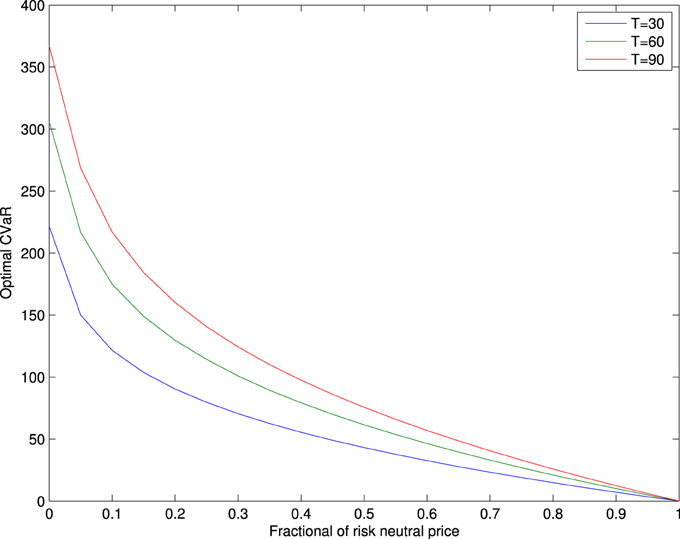
Figure 1. Optimal CVaRs against hedging costs.

FIGURE 2

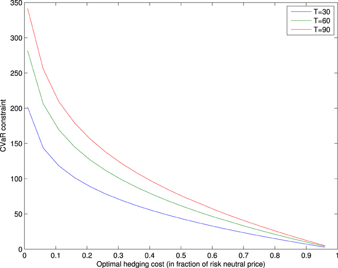
Figure 2. Optimal hedging costs against CVaR.

Figure 1 plots the optimal CVaRs with respect to the constraint on the initial costs ν, which is given by the fraction of the risk neutral price. One can observe that the optimal CVaRs decrease to zero when ν equals to the risk neutral price, meaning that the call option is hedged perfectly. CVaRs reach to the maximum values when the fraction equals to zero, implying that the investor is exposed to the full risk. The optimal CVaR comes near zero when the allocation of initial wealth approaches to the risk neutral price in the case of perfect hedging. The optimal CVaRs also increases as the the maturity T increases, showing that the risk is larger for portfolios held longer.

Figure 2 plots the optimal hedging costs according to the constraint c on CVaR. We can see that Figure 2 demonstrates similar trends as in Figure 1. When c reaches to 350, the resulting risk is close the the maximum CVaR in Figure 1, and its corresponding optimal hedging cost equals to zero. When the CVaR value is fixed at zero, we obtain the perfect hedging. The minimal optimal hedge equals to the risk neutral price.

5. Conclusion

The purpose of this paper is to construct CVaR hedging strategies under stochastic interest rate environment. We first generalize the results presented by Melnikov and Smirnov [7], and then add the stochastic interest rate component. Modeling the stochastic movements of interest rates is essential in pricing and hedging interest-rate-sensitive price; the result of this paper can be applied on pricing a variety of equity-linked life insurance products, for example. The Neyman Pearson lemma shows that the optimal strategy of CVaR hedging is a perfect hedge for an adjusted claim.

To illustrate this hedging technique we consider a European call option, explicit formulas for solving CVaR minimization problems under HJM framework are derived. Note that the geometric Brownian motion is employed in monitoring the asset dynamics. As the risk of Brownian motion is completely determined by its variance, the advantage of CVaR is not shown in this thin-tailed model. For future work we consider improving CVaR hedging by adopting heavy-tailed models and adding jump components.

Author Contributions

Three authors contributed significantly to all aspects of this work.

Conflict of Interest Statement

The authors declare that the research was conducted in the absence of any commercial or financial relationships that could be construed as a potential conflict of interest.

Acknowledgments

Many thanks to Professor Svetlozar Rachev for stimulating discussions. Without his help, this paper could not be finished.

References

1. Föllmer H, Leukert P. Quantile hedging. Finance Stochast. (1999) 3:251–73. doi: 10.1007/s007800050062

CrossRef Full Text | Google Scholar

2. Föllmer H, Leukert P. Efficient hedging: cost versus shortfall risk. Finance Stochast. (2000) 4:117–46. doi: 10.1007/s007800050008

CrossRef Full Text | Google Scholar

3. Krutchenko R, Melnikov A. Quantile hedging for a jump-diffusion financiall market model. In: Kohlmann M, editor. Trends in Mathematics. Basel/Switzerland: Birkhauser-Verlag (2001).

4. Melnikov A. Quantile hedging of equity-linked life insurance policies. Dokl Akad Nauk. (2004) 396:601–3.

Google Scholar

5. Melnikov A, Romanyuk Y. Efficient hedging and pricing of equity-linked life insurance contracts on several assets. Int J Theor Appl Finance. (2008) 11:295–323. doi: 10.1142/S0219024908004816

CrossRef Full Text | Google Scholar

6. Melnikov A, Skornyakova V. Quantile hedging and its application to life insurance. Stat Decis Int J Stochast Methods Models. (2005) 23:301–16. doi: 10.1524/stnd.2005.23.4.301

CrossRef Full Text | Google Scholar

7. Melnikov A, Smirnov I. Dynamic hedging of conditional value-at-risk. Insurance (2012) 51:182–190. doi: 10.1016/j.insmatheco.2012.03.011

CrossRef Full Text | Google Scholar

8. Heath D, Jarrow R, Morton A. Bond and pricing the term structure of interest rates: a new methodology for contingent claims valuation. Econometrica (1992) 60:77–105. doi: 10.2307/2951677

CrossRef Full Text | Google Scholar

9. Ciurlia P, Gheno A. A model for pricing real estate derivatives with stochastic interest rates. Math Comput Model. (2009) 50:233–47. doi: 10.1016/j.mcm.2008.12.005

CrossRef Full Text | Google Scholar

10. Jalen L, Mamon R. Valuation of contingent claims with mortality and interest rate risks. Math Comput Model. (2009) 49:1893–904. doi: 10.1016/j.mcm.2008.10.014

CrossRef Full Text | Google Scholar

11. Gao Q, He T, Zhang C. Quantile hedging for equity-linked life insurance contracts in a stochastic interest rate economy. Econ Model. (2011) 28:147–56. doi: 10.1016/j.econmod.2010.09.016

CrossRef Full Text | Google Scholar

12. Black F, Scholes M. The pricing of options and corporate liabilities. J Polit Econ. (1973) 81, 637–54. doi: 10.1086/260062

PubMed Abstract | CrossRef Full Text | Google Scholar

13. Merton RC. Option pricing when underlying stock returns are discontinuous. J Financ Econ. (1976) 3:125–44. doi: 10.1016/0304-405X(76)90022-2

CrossRef Full Text | Google Scholar

14. Rockafellar RT, Uryasev S. Optimization of conditional value-at-risk. J Risk. (2000) 2:21–42. Available online at: http://www.ise.ufl.edu/uryasev/files/2011/11/CVaR1_JOR.pdf.

15. Föllmer H, Schied A, Lyons TJ. Stochastic Finance. An Introduction in Discrete Time. Berlin: Springer (2004).

16. Amin KI, Jarrow RA. Pricing options on risky assets in a stochastic interest rate economy. Math Finance. (1992) 2:217–37. doi: 10.1111/j.1467-9965.1992.tb00030.x

CrossRef Full Text | Google Scholar

17. Park F. Implementing Interest Rate Models: A Practical Guide. Capital Markets and Portfolio Research (CMPR) (2004).

Google Scholar

Appendix

Appendix A. Calculation of Equation (14)

Here we review the valuation of European call option under HJM model. Recall that the price of the option is given by:

$\begin{array}{l}{V}_0=E^{\mathbb{Q}}[R{(T)}^{-1}{(S(T)-K)}^{+}]\\ =E^{\mathbb{Q}}[R{(T)}^{-1}S(T)1_{\{S(T)>K\}}]-E^{\mathbb{Q}}[R{(T)}^{-1}K{1}_{\{S(T)>K\}}].\end{array}$

First define

$\begin{array}{l}\frac{d{\mathbb{Q}}_1}{d\mathbb{Q}}:=\exp (-\frac{1}{2}{\displaystyle {\int }_0^T\left({\sigma }_1{\left(u\right)}^2+{\sigma }_2{\left(u\right)}^2\right)}du+\\ {\displaystyle {\int }_0^T{\sigma }_1}\left(u\right)d{B}_1^{\mathbb{Q}}\left(u\right)+{\displaystyle {\int }_0^T{\sigma }_2}\left(u\right)d{B}_2^{\mathbb{Q}}\left(u\right)),\end{array}$

then under we have

$\begin{array}{ll}{B}_1^{\mathbb{Q}}(t)=B_1^{{\mathbb{Q}}_1}(t)+{\displaystyle {\int }_0^t{\sigma }_1}(u)du,\hfill & (\text{A}1)\hfill \end{array}$

$\begin{array}{ll}{B}_2^{\mathbb{Q}}(t)=B_2^{{\mathbb{Q}}_1}(t)+{\displaystyle {\int }_0^t{\sigma }_2}(u)du,\hfill & (\text{A}2)\hfill \end{array}$

where Bℚ11 and Bℚ12 are two independent Brownian motions under ℚ1. Thus,

$\begin{array}{l}S(T)=S\left(0\right)R\left(T\right)\exp (-\frac{1}{2}{\displaystyle {\int }_0^T\left({\sigma }_1{\left(u\right)}^2+{\sigma }_2{\left(u\right)}^2\right)}du+\\ {\displaystyle {\int }_0^T{\sigma }_1}\left(u\right)d{B}_1^{\mathbb{Q}}\left(u\right)+{\displaystyle {\int }_0^T{\sigma }_2}\left(u\right)d{B}_2^{\mathbb{Q}}\left(u\right))\\ =\frac{S\left(0\right)}{P\left(0,T\right)}\exp (\frac{1}{2}{\displaystyle {\int }_0^T{\left({\sigma }^{*}(u,T)+{\sigma }_1\left(u\right)\right)}^2+}\\ {\sigma }_2{\left(u\right)}^2)du+{\displaystyle {\int }_0^T\left({\sigma }^{*}(u,T)+{\sigma }_1\left(u\right)\right)}d{B}_1^{{\mathbb{Q}}_1}(u)+\\ {\displaystyle {\int }_0^T{\sigma }_2}\left(u\right)d{B}_2^{{\mathbb{Q}}_1}\left(u\right)).\end{array}$

The event S(T) > K implies that

$\begin{array}{l}{\displaystyle {\int }_0^T\left({\sigma }^{*}(u,T)+{\sigma }_1(u)\right)}d{B}_1^{{\mathbb{Q}}_1}(u)+{\displaystyle {\int }_0^T{\sigma }_2}(u)d{B}_2^{{\mathbb{Q}}_1}(u)\\ >\log \left(\frac{P(0,T)K}{S(0)}\right)-\frac{1}{2}{\displaystyle {\int }_0^T\left({({\sigma }^{*}(u,T)+{\sigma }_1(u))}^2+{\sigma }_2{(u)}^2\right)}du.\end{array}$

Thus, we have

$E^{\mathbb{Q}}[R{(T)}^{-1}S(T)1_{\{S(T)>K\}}]=S(0)E^{{\mathbb{Q}}_1}[1_{\{S(T)>K\}}]=S(0)N(d_1),$

where d₁ is given by Equation (15). On the other side, define

$\frac{d{\mathbb{Q}}_2}{d\mathbb{Q}}:=\exp \left(-{\displaystyle {\int }_0^T{\sigma }^{*}}(u,T)d{B}_1^{\mathbb{Q}}(u)-\frac{1}{2}{\displaystyle {\int }_0^T{\sigma }^{*}}{(u,T)}^{2}du\right),$

Then we have

$\begin{array}{ll}{B}_1^{\mathbb{Q}}(t)=B_1^{{\mathbb{Q}}_2}(t)-{\displaystyle {\int }_0^t{\sigma }^{*}}(u,T)du\hfill & (\text{A}3)\hfill \end{array}$

$\begin{array}{ll}{B}_2^{\mathbb{Q}}(t)=B_2^{{\mathbb{Q}}_2}(t)\hfill & (\text{A}4)\hfill \end{array}$

where Bℚ21 and Bℚ22 are two independent Brownian motions under ℚ2. Thus,

$\begin{array}{l}S(T)=\frac{S(0)}{P(0,T)}\exp (-\frac{1}{2}\text{}{\displaystyle {\int }_0^T\left({\left({\sigma }^{*}(u,T)+{\sigma }_1(u)\right)}^2\text{}+{\sigma }_2{(u)}^2\right)}du\\ +{\displaystyle {\int }_0^t\left({\sigma }^{*}(u,T)+{\sigma }_1(u)\right)d{B}_1^{{\mathbb{Q}}_2}(u)+{\displaystyle {\int }_0^t{\sigma }_2}\left(u\right)d{B}_2^{{\mathbb{Q}}_2}\left(u\right)}).\end{array}$

The event S(T) > K implies that

$\begin{array}{l}{\displaystyle {\int }_0^T({\sigma }^{*}(u,T)+{\sigma }_1(u))d{B}_1^{{\mathbb{Q}}_2}(u)+{\displaystyle {\int }_0^T{\sigma }_2}(u)d{B}_2^{{\mathbb{Q}}_2}(u)}\\ >\log \left(\frac{P(0,T)K}{S(0)}\right)+\frac{1}{2}{\displaystyle {\int }_0^T\left({\left({\sigma }^{*}(u,T)+{\sigma }_1(u)\right)}^2+{\sigma }_2{(u)}^2\right)}du.\end{array}$

Then

$E^{\mathbb{Q}}[R{(T)}^{-1}K{1}_{\{S(T)>K\}}]=KP(0,T)N(d_2)$

where d₂ is given by Equation (16).

Appendix B. Calculation of Equation (17)

We can decompose f^call₁ to be:

$\begin{array}{l}{f}_1^{call}(z,a)=E^{\mathbb{Q}}[R{(T)}^{-1}{(S(T)-K-z)}^{+}{1}_{\{R(T)\frac{d\mathbb{P}}{d\mathbb{Q}}>a\}}]\\ =S(0)E^{{\mathbb{Q}}_1}[1_{\{S(T)>K+z\}}{1}_{\{R(T)\frac{d\mathbb{P}}{d\mathbb{Q}}>a\}}]-\\ (K+z)P(0,T)E^{{\mathbb{Q}}_2}[1_{\{S(T)>K+z\}}{1}_{\{R(T)\frac{d\mathbb{P}}{d\mathbb{Q}}>a\}}],\end{array}$

where ℚ₁ and ℚ₂ are defined in the previous section. Then apply Equations (A1) and (A2) we obtain the dynamic of R(T)dℙ/dℚ under ℚ₁:

$\begin{array}{l}R(T)\frac{d\mathbb{P}}{d\mathbb{Q}}=\frac{1}{P(0,T)}\exp (\frac{1}{2}{\displaystyle {\int }_0^T\left({\sigma }^{\ast }{(u,T)}^2-{\theta }_1{(u)}^2-{\theta }_2{(u)}^2\right)}\\ du+{\displaystyle {\int }_0^T\left({\sigma }^{*}(u,T)-{\theta }_1(u)\right)d{B}_1^{\mathbb{Q}}(u)}\\ -{\displaystyle {\int }_0^T{\theta }_2}(u)d{B}_2^{\mathbb{Q}}(u))\\ =\frac{1}{P(0,T)}\exp \left({\Sigma }_{12}-\frac{1}{2}{\Sigma }_{11}-W_1\right),\end{array}$

where Σ₁₁, Σ₁₂ are given by Equations (20, 22), and

$W_1{:}^{\underset{\_}{\underset{\_}{d}}}{\displaystyle {\int }_0^T({\theta }_1(u)-{\sigma }^{*}(}u,T))d{B}_1^{{\mathbb{Q}}_1}(u)+{\displaystyle {\int }_0^T{\theta }_2}(u)d{B}_2^{{\mathbb{Q}}_1}(u)$

Therefore, R(T)dℙ/dℚ > a implies

$W_1<-\log (aP(0,T))+{\Sigma }_{12}-\frac{1}{2}{\Sigma }_{11}.$

On the other side, recall S(T) > K + z implies

$\begin{array}{l}{\text{W}}_2:\stackrel{d}{=}-{\displaystyle {\int }_0^T({\sigma }^{*}(}u,T)+{\sigma }_1(u))d{B}_1^{{\mathbb{Q}}_1}(u)-{\displaystyle {\int }_0^T{\sigma }_2}(u)d{B}_2^{{\mathbb{Q}}_1}(u)\\ <\log \left(\frac{S(0)}{P(0,T)(K+z)}\right)+\frac{1}{2}{\displaystyle {\int }_0^T(({\sigma }^{*}(u,T)+}\\ {{\sigma }_1(u))}^2+{\sigma }_2{(u)}^2)du\\ =\log \left(\frac{S(0)}{P(0,T)(K+z)}\right)+\frac{1}{2}{\Sigma }_{22},\end{array}$

where Σ₂₂ is given by Equation (21). Note that (W₁, W₂) are binormal distributed with zero mean and covariance matrix Σ. It is easy to compute that the entries of Σ

$\begin{array}{l}{\Sigma }_{11}=E[W_1^2]={\displaystyle {\int }_0^T((}{\theta }_1(u)-{\sigma }^{\ast }(u,T){)}^2\\ +{\theta }_2{(u)}^2)du,\\ {\Sigma }_{22}=E[W_2^2]={\displaystyle {\int }_0^T({\sigma }^{*}(}u,T)+{\sigma }_1(u){)}^2\\ +{\sigma }_2{(u)}^{2}du,\\ {\Sigma }_{12}={\Sigma }_{21}=E[W_1{W}_2]=-{\displaystyle {\int }_0^T({\theta }_1(u)-{\sigma }^{*}(}u,T))\\ ({\sigma }^{\ast }(u,T)+{\sigma }_1(u))du-{\displaystyle {\int }_0^T{\theta }_2}(u){\sigma }_2(u)du.\end{array}$

Thus, we have:

$S(0)E^{{\mathbb{Q}}_1}[1_{\{S(T)>K+z\}}{1}_{\{R(T)\frac{d\mathbb{P}}{d\mathbb{Q}}>c\}}]=S(0)N_2({\Sigma }^{-1/2}{\eta }_1(z,a)),$

where η₁(z, a) is given by Equation (18). Similarly under ℚ₂ we have

$\begin{array}{l}R(T)\frac{d\mathbb{P}}{d\mathbb{Q}}=\frac{1}{P(0,T)}\exp (-\frac{1}{2}{\displaystyle {\int }_0^T({\left({\theta }_1(u)-{\sigma }^{*}(u,T)\right)}^2+}\\ {\theta }_2{(u)}^2)du+{\displaystyle {\int }_0^T\left({\sigma }^{*}(u,T)-{\theta }_1(u)\right)d{B}_1^{{\mathbb{Q}}_2}(u)-}\\ {\displaystyle {\int }_0^T{\theta }_2}(u)d{B}_2^{{\mathbb{Q}}_2}(u))\\ =\frac{1}{P(0,T)}\exp \left(-\frac{1}{2}{\Sigma }_{11}-W_1\right),\end{array}$

and that R(T)dℙ/dℚ > a implies

$W_1<-\log (aP(0,T))-\frac{1}{2}{\Sigma }_{11}.$

And recall that S(T) > K + z implies

$\begin{array}{l}{W}_2<\log \left(\frac{S(0)}{P(0,T)(K+z)}\right)-\frac{1}{2}{{\displaystyle {\int }_0^T(\left({\sigma }^{*}(u,T)+{\sigma }_1(u)\right)}}^2\\ +{\sigma }_2{(u)}^2)du\\ =\log \left(\frac{S(0)}{P(0,T)(K+z)}\right)-\frac{1}{2}{\Sigma }_{22}.\end{array}$

Note that here we keep use (W₁, W₂) to denote a bivariate normal random vector under ℚ₂ instead of ℚ₁ for simplicity. Thus, we have

$\begin{array}{l}(K+z)P(0,T)E^{{\mathbb{Q}}_2}[1_{\{S(T)>K+z\}}{1}_{\{R(T)\frac{d\mathbb{P}}{d\mathbb{Q}}>c\}}]=(K+z)\\ P(0,T)N_2({\Sigma }^{-1/2}{\eta }_2(z,a)),\end{array}$

where η₂(z, a) is given by Equation (19).

Appendix C. Calculation of Equation (23)

Recall that the dynamic of stock price process under market measure ℙ is given by

$\begin{array}{l}S(t)=S(0)R(t)\exp ({\displaystyle {\int }_0^t\left(\mu (u)-\frac{1}{2}({\sigma }_1{(u)}^2+{\sigma }_2{(u)}^2)\right)}du+\\ {\displaystyle {\int }_0^t{\sigma }_1}(u)d{B}_1^{\mathbb{P}}(u)+{\displaystyle {\int }_0^t{\sigma }_2}(u)B_2^{\mathbb{P}}(u))\\ =\frac{S(0)}{P(0,t)}\exp ({\displaystyle {\int }_0^t(\mu (u)+{\alpha }^{*}(u,t)-\frac{1}{2}({\sigma }_1{(u)}^2+}\\ {\sigma }_2{(u)}^2))du\\ +{\displaystyle {\int }_0^t({\sigma }^{*}(}u,t)+{\sigma }_1(u))d{B}_1^{\mathbb{P}}(u)+{\displaystyle {\int }_0^t{\sigma }_2}(u)B_2^{\mathbb{P}}(u)).\end{array}$

Consider the decomposition of f^call₂:

$\begin{array}{l}{f}_2^{call}(z,a)=E^{\mathbb{P}}[S(T)1_{\{S(T)>K+z\}}{1}_{\{R(T)\frac{d\mathbb{P}}{d\mathbb{Q}}\le a\}}]-\\ (K+z)E^{\mathbb{P}}[1_{\{S(T)>K+z\}}{1}_{\{R(T)\frac{d\mathbb{P}}{d\mathbb{Q}}\le a\}}].\end{array}$

Here to define a new measure $\tilde{\mathbb{P}}$:

$\begin{array}{l}\frac{d\tilde{\mathbb{P}}}{d\mathbb{P}}:=\exp ({\displaystyle {\int }_0^T({\sigma }^{*}(u,T)+{\sigma }_1(u))d{B}_1^{\mathbb{P}}(u)+{\displaystyle {\int }_0^T{\sigma }_2}(u)B_2^{\mathbb{P}}(u)-}\\ \frac{1}{2}{\displaystyle {\int }_0^T({\sigma }^{*}(}u,T)+{\sigma }_1(u){)}^2+{\sigma }_2{(u)}^2)du).\end{array}$

Then we have

$\begin{array}{l}{E}^{\mathbb{P}}[S(T)1_{\{S(T)>K+z\}}{1}_{\{R(T)\frac{d\mathbb{P}}{d\mathbb{Q}}\le a\}}]=\frac{S(0)}{P(0,T)}{e}^A{E}^{\tilde{\mathbb{P}}}[1_{\{S(T)>K+z\}}\\ 1_{\{R(T)\frac{d\mathbb{P}}{d\mathbb{Q}}\le a\}}],\end{array}$

where A is given by Equation (26). By Girsanov theorem we have

$\begin{array}{l}{B}_1^{\mathbb{P}}(t)=B_1^{\tilde{\mathbb{P}}}(t)+{\displaystyle {\int }_0^t({\sigma }^{*}(}u,T)+{\sigma }_1(u))du,\\ B_2^{\mathbb{P}}(t)=B_2^{\tilde{\mathbb{P}}}(t)+{\displaystyle {\int }_0^t{\sigma }_2}(u)du.\end{array}$

where B^{$\tilde{\mathbb{P}}$}₁ and B^{$\tilde{\mathbb{P}}$}₂ are two independent Brownian motions under $\tilde{\mathbb{P}}$. Then S(T) and R(T)dℙ/ℚ becomes:

$\begin{array}{l}S(T)=\frac{S(0)}{P(0,T)}\exp ({\displaystyle {\int }_0^T(\mu (u)+{\alpha }^{*}(u,T)-\frac{1}{2}({\sigma }_1{(u)}^2+}\\ {\sigma }_2{(u)}^2))\\ du+{\displaystyle {\int }_0^T({\sigma }^{*}(}u,T)+{\sigma }_1(u))d{B}_1^{\mathbb{P}}(u)+\\ {\displaystyle {\int }_0^T{\sigma }_2}(u)B_2^{\mathbb{P}}(u))\\ =\frac{S(0)}{P(0,T)}\exp \left(A+\frac{1}{2}{\Sigma }_{22}-W_2\right),\end{array}$

and

$\begin{array}{l}R(T)\frac{d\mathbb{P}}{d\mathbb{Q}}=\frac{1}{P(0,T)}\exp ({\displaystyle {\int }_0^T({\alpha }^{*}(u,T)+\frac{1}{2}({\theta }_1{(u)}^2+}\\ {\theta }_2{(u)}^2))\\ du-{\displaystyle {\int }_0^T({\theta }_1(u)-{\sigma }^{*}(}u,T))d{B}_1^{\mathbb{P}}(u)-\\ {\displaystyle {\int }_0^T{\theta }_2}(u)d{B}_2^{\mathbb{P}}(u))\\ =\frac{1}{P(0,T)}\exp \left(A+\frac{1}{2}{\Sigma }_{11}-W_1\right)\end{array}$

Thus, R(T)dℙ/dℚ ≤ a implies

$-W_1\le \log (aP(0,T))-A-\frac{1}{2}{\Sigma }_{11},$

and S(T) > K + z implies

$W_2<\log \left(\frac{S(0)}{P(0,T)(K+z)}\right)+A+\frac{1}{2}{\Sigma }_{22}.$

It is easy to see that (W₁, W₂) ~ N(0, $\tilde{\Sigma }$). Then we have

$E^{\mathbb{P}}[S(T)1_{\{S(T)>K+z\}}{1}_{\{R(T)\frac{d\mathbb{P}}{d\mathbb{Q}}\le a\}}]=\text{}\frac{S(0)}{P(0,T)}{e}^A{N}_2({\tilde{\Sigma }}^{-1/2}{\zeta }_1(z,a)),$

where ζ₁(z, a) is given by Equation (24). On the other side we do not need to change the measure. For {R(T)dℙ/dℚ ≤ a} we have

$\begin{array}{l}-W_1\le \log (aP(0,T))-\\ {\displaystyle {\int }_0^T\left({\alpha }^{*}(u,T)+\frac{1}{2}({\theta }_1{(u)}^2+{\theta }_2{(u)}^2)\right)}du,\end{array}$

and for S(T) > K + z we have

$\begin{array}{l}{W}_2<\log \left(\frac{S(0)}{P(0,T)(K+z)}\right)+{\displaystyle {\int }_0^T(\mu (u)+{\alpha }^{*}(u,T)}\\ -\frac{1}{2}({\sigma }_1{(u)}^2+{\sigma }_2{(u)}^2))du.\end{array}$

Finally we will get

$(K\text{}+\text{}z)E^{\mathbb{P}}[1_{\{S(T)>K+z\}}{1}_{\{R(T)\frac{d\mathbb{P}}{d\mathbb{Q}}\le a\}}]=(K+z)N_2({\tilde{\Sigma }}^{-1/2}{\zeta }_2(z,a)),$

where ζ₂(z, a) is given by Equation (25).