Investing in Global Markets: Big Data and Applications of Robust Regression

Investing in Global Markets: Big Data, Outliers, and Robust Regression

In this study, we apply robust regression techniques to model stock returns and create stock selection models in a very large global stock universe. We employ Markowitz portfolio construction and optimization techniques to a global stock universe. We estimate expected return models in the global market using a given stock selection model and generate statistically significant active returns from various portfolio construction techniques. In the first section, we introduce the reader to the risk and return trade-off analysis. In second section, we introduce the reader to modeling expected returns and make extensive use of robust regression techniques. In the third section, we examine the relationship of the (traditional) Markowitz mean-variance (MV) portfolio construction model with a fixed upper bound on security weights. In fourth section, we discuss portfolio construction and simulation, and present the empirical results. In fifth section, we offer conclusions and a summary. We report that mean-variance techniques using robust regression-created expected returns continue to produce portfolios capable of generating excess returns above transactions costs and statistically significant asset selection in a global stock market offer the potential for high returns relative to risk. The stock selection model used in this analysis is the “public form” of the McKinley Capital Management proprietary model. The public form model produces highly statistically significant asset selection and similar factor risk exposures to our proprietary model.

Introduction

Markowitz developed a portfolio construction model to achieve the maximum return for a given level of risk or the minimum risk for a given level of return (1952, 1959, 1976, and 2013). We create a global set of portfolios over the 1997–2014 time period that offer substantial outperformance of a global stock benchmark by using Beaton and Tukey [1], Gunst et al. [2], Gunst and Mason [3], Rousseeuw [4], Rousseeuw and Hubert [5], Rousseeuw and Leroy [6], Rousseeuw and Yohai [7], and Yohai et al. [8] MM robust regression techniques, discussed in Maronna et al. [9], to create expected returns and a mean-variance tracking error at risk (MVTaR) portfolio construction technique. The regression models used to create expected returns combine well-established fundamental factors, such as earnings, book value, cash flow, and sales, forecasted earnings acceleration, and price momentum factors. Robust regression models are used to estimate the determinants of total stock returns. The regression techniques in this study include the Beaton-Tukey [1] Bisquare weighting procedure that produces regression weights for data¹. The reader is referred to Bloch et al. [12], Guerard et al. [13], and Guerard et al. [14]. These factors are statistically significant in univariate models (tilts) and in multiple-factor models (MFM). We briefly review the applied U.S. and Global equity investment research in Guerard et al. [15], Guerard et al. [13], and Guerard et al. [14]. We test whether a mean-variance optimization technique using the portfolio variance as the relevant risk measure dominates the risk-return trade-off curve using a variation of the optimization model that emphasizes systematic (or market) risk. A statistically-based Principal Components Analysis (PCA) model is used to estimate and monitor portfolio risk.

A measure of the trade-off between the portfolio expected return and risk (as measured by the portfolio standard deviation) is typically denoted by the Greek letter lambda (λ). Generally, the higher the lambda, the higher is the ratio of portfolio expected return to portfolio standard deviation. We assume that the portfolio manager seeks to maximize the portfolio geometric mean (GM) and Sharpe ratio (ShR) as put forth in Latane et al. [16] and Markowitz [17, 18]. The reader is referred to Elton et al. [19] for a complete discussion of modern portfolio theory.

Regression-Based Expected Returns Modeling

In 1991, Markowitz headed the Daiwa Securities Trust Global Portfolio Research Department (GPRD). The Markowitz team estimated stock selection models, following in the tradition of Graham and Dodd [20], Williams [21], Basu [22], Guerard and Stone [23], Dimson [24], and Haugen and Baker [25], who tested fundamental valuation variables, earnings, book value, cash flow, and sales. The Markowitz team used relative variables, defined as the ratio of the absolute fundamental variable ratios divided by the 60-month averages of the fundamental variables. Bloch et al. [12] reported a set of ~200 simulations of United States and Japanese equity models. The models produced out-of-sample statistically significant excess returns in the portfolios. Guerard et al. [15] extended a stock selection model originally developed and estimated in Bloch et al. [12] by adding price momentum variable, taking the price at time t-1 divided by the price 12 months ago, t-12, denoted PM, and the consensus (I/B/E/S) analysts' earnings forecasts and analysts' revisions composite analysts' efficiency variable (CTEF) to the stock selection model. Guerard [26] used the CTEF variable that is composed of forecasted earnings yield, EP, revisions, EREV, and direction of revisions, EB, identified as breadth, as created in Guerard et al. [27]². Guerard also reported domestic (U.S.) evidence that the predicted earnings yield is incorporated into the stock price through the earnings yield risk index. Moreover, CTEF dominates the historic low price-to-earnings effect, or high earnings-to-price, EP. Fama and French [28–30] presented evidence to support the BP and price momentum variables as anomalies. Levy [31], Chan et al. [32], Conrad and Kaul [33, 34], Jegadeesh and Titman [35], Sadka [36], and Korajczyk and Sadka [37] present the academic evidence to support the price momentum hypothesis that past winners continue to win and past losers continue to lose. Brush and Boles [38] and Brush [39, 40] present the practitioner-oriented evidence to support price momentum.

Guerard et al. [15] referred to the stock selection model as a United States Expected Returns (USER) Model. Guerard et al. [13] applied the USER Model a large set of global stocks for the 1997–2011 time period. Guerard et al. [13] refereed to the global expected returns model as the GLER Model. We can estimate an expanded stock selection model to use as an input of expected returns in an optimization analysis.

The stock selection model estimated in this study, denoted as GLER is:

$\begin{array}{cc}\begin{array}{l}T{R}_{t+1}=a_0+a_{1}E{P}_t+a_{2}B{P}_t+a_{3}C{P}_t+a_{4}S{P}_t+a_{5}RE{P}_t\\ +a_6{\text{RBP}}_t+a_{7}RC{P}_t+a_{8}RS{P}_t+a_{9}CTE{F}_t\\ +a_{10}P{M}_t+e_t\end{array}& \left(1\right)\end{array}$

where:

TR = total stock returns;

EP = [earnings per share]/[price per share] = earnings-price ratio;

BP = [book value per share]/[price per share] = book-price ratio;

CP = [cash flow per share]/[price per share] = cash flow-price ratio;

SP = [net sales per share]/[price per share] = sales-price ratio;

REP = [current EP ratio]/[average EP ratio over the past 5 years];

RBP = [current BP ratio]/[average BP ratio over the past 5 years];

RCP = [current CP ratio]/[average CP ratio over the past 5 years];

RSP = [current SP ratio]/[average SP ratio over the past 5 years];

CTEF = consensus earnings per share I/B/E/S forecast, revisions and breadth;

PM = Price Momentum;

and

e = randomly distributed error term.

The GLER model is estimated using a weighted latent root regression (WLRR), analysis on Equation (1) to identify variables statistically significant at the 10% level; uses the normalized coefficients as weights; and averages the variable weights over the past 12 months. The 12-month smoothing is consistent with the four-quarter smoothing in Bloch et al. [12]. While EP and BP variables are significant in explaining returns, the majority of the forecast performance is attributable to other model variables, namely the relative earnings-to-price, relative cash-to-price, relative sales-to-price, price momentum, and earnings forecast variables. The CTEF and PM variables accounted 40% of the weights in the GLER Model. We refer to using WLRR on the first eight variables, the Markowitz Model, as REG8F WLRR. Many statisticians prefer to describe this formulation as the bisquare, or biweight function, see Maronna et al. [9].

One can estimate in Equation (1) using ordinary least squares, using multiple regression.

$\begin{array}{cc}\widehat{\beta }=(\text{X}\prime \text{X})\text{X}\prime \text{Y}& \left(2\right)\end{array}$

The residuals of the multiple regression line is given by:

$\text{e}=\text{Y}\prime -\widehat{\beta }\text{X}$

The regressions residuals are assumed to be independently and identically distributed variables.

Bloch et al. [12] employed the Beaton-Tukey Bisquare procedure to weight observations identified as outliers. There are several methods that one can use to identify influential observations or outliers, which are often referred to as an analysis of influential observations³. Belsley et al. [41], showed that the estimated regression coefficients change by an amount, DFBETA, where:

$\begin{array}{cc}DFBET{A}_i=\frac{{(\text{X}\prime \text{X})}^{-1}\text{X}\prime e_i}{1-h_i}& \left(3\right)\end{array}$

where $h_i={\text{X}}_i{({\text{X}}^{\prime }\text{X})}^{-1}{\text{X}}_i^{\prime }$

The h_i or “hat,” term is calculated by deleting observation i. The corresponding residual is known as the studentized residual, sr, and defined as:

$\begin{array}{cc}s{r}_i=\frac{e_i}{\widehat{\sigma }\sqrt{1-h_i}}& \left(4\right)\end{array}$

where $\widehat{\sigma }$ is the estimated standard deviation of the residuals. A studentized residual that exceeds 2.0 indicates a potential influential observation [41]⁴. As the researcher or modeler deletes observations, one needs to compare the original matrix of the estimated residuals variance matrix. The COVRATIO calculation performs this calculation, where:

$\begin{array}{cc}COVRATIO=\frac{1}{{\left[\frac{n-p-1}{n-p}+\frac{e_i^{\ast }}{(n-p)}\right]}^p(1-h_i)}& \left(5\right)\end{array}$

where n = number of observations,

p = number of independent variables,

and e${}_{\text{i}}^{*}=$ deleted observations.

If the absolute value of the deleted observation >2, then the COVRATIO calculation approaches:

$\begin{array}{cc}1-\frac{3p}{n}& \left(6\right)\end{array}$

A calculated COVRATIO that is larger than 3p/n indicates an influential observation. Guerard [26] reported the usefulness of the DFBETA, studentized residual, CookD, and COVRATIO calculations performed with SAS and the GLER data during the 1997–2011 time period⁵. In robust regression one weights the data universally with its OLS residual; i.e., the larger the residual, the smaller the weight of the observation in the robust regression. In robust regression, several weights may be used.

We will review the Beaton-Tukey [1] bisquare weighting scheme, where observations are weighted inversely with their corresponding ordinary least squares residual, w:

where:

$\begin{array}{cc}\begin{array}{l}{w}_i={\left(1-{\left(\frac{\frac{\left|e_i\right|}{{\sigma }_e}}{4.685}\right)}^2\right)}^2,if\frac{\left|e_i\right|}{{\sigma }_e}>4.685;\hfill \\ 1,if\frac{\left|e_i\right|}{{\sigma }_e}<\mathrm{4.685.}\hfill \end{array}& \left(7\right)\end{array}$

A second major problem is one of multicollinearity, the condition of correlations among the independent variables. If the independent variables are perfectly correlated in multiple regression, then the (X′X) matrix of Equation (1), cannot be inverted and the multiple regression coefficients have multiple solutions. In reality, highly correlated independent variables can produce unstable regression coefficients due to an unstable (X′X)⁻¹ matrix. Belsley et al. advocate the calculation of a condition number, which is the ratio of the largest latent root of the correlation matrix relative to the smallest latent root of the correlation matrix. A condition number exceeding 30.0 indicates severe multicollinearity.

The latent roots of the correlation matrix of independent variables can be used to estimate regression parameters in the presence of multicollinearity. The latent roots, l₁, l₂, …, l_p and the latent vectors γ₁, γ₂, …  γ_p of the P independent variables can describe the inverse of the independent variable matrix of Equation (1). The models produced out-of-sample statistically significant excess returns in the portfolios.

$\begin{array}{cc}{(\text{X}\prime \text{X})}^{-1}={\displaystyle \sum _{j=1}^p{l}_j^{-1}}{\gamma }_j{\gamma }_j^{\prime }& \left(8\right)\end{array}$

Multicollinearity is present when one observes one or more small latent vectors. If one eliminates latent vectors with small latent roots (l < 0.30) and latent vectors (γ < 0.10), the “principal component” or latent root regression estimator may be written as:

$\begin{array}{cc}{\widehat{\beta }}_{LRR}={\displaystyle \sum _{j=0}^P{f}_j}{\delta }_j& \left(9\right)\end{array}$

$\begin{array}{cc}\begin{array}{l}\text{where}{f}_j=\frac{-\eta {\gamma }_0{\lambda }_j^{-1}}{{\displaystyle {\sum }_q{\gamma }_0^2}{\lambda }_q^{-1}}\\ \text{where}{\text{n}}^2=\Sigma {\left(y-\overline{y}\right)}^2\end{array}& \left(10\right)\end{array}$

and λ are the “non-zero” latent vectors. One eliminates the latent vectors with non-predictive multicollinearity. Guerard et al. [13] reported the effective ness of the WLRR models that made extensive use of outlier-induced collinearities, originally formulated in Webster et al. [43], Gunst and Mason [44], Mason and Gunst [45], and Carrillo-Gambos and Gunst [46].

Maronna et al. [9] surveyed robust statistics. Considerable attention was paid to the MM-estimates techniques pioneered by Yohai [47], Yohai and Zamar [48], and Yohai et al. [8]. The MM estimates used a high break point, often low normal efficient estimate with a robust scale of residuals, and iterated to produce high break point and efficient estimates, see Ruppert [49] for modeling with residual scaling. We refer to using MM-estimation, on the first eight variables (the Markowitz Model), using the Yohai-optimal influence function, as REG8-Optimal. We refer to using MM-estimation, using all 10 variables and the Yohai-optimal function, as REG10-Optimal. We report both WLRR and Yohai's optimal function MM-Method estimates in Section The Data and Empirical Results.

Constructing Mean-Variance Efficient Portfolios

Portfolio construction and management, as formulated in Markowitz seeks to identify the efficient frontier, the point at which the portfolio return is maximized for a given level of risk, or equivalently, portfolio risk is minimized for a given level of portfolio return. The portfolio expected return, denoted by E(R_P), is calculated by taking the sum of the security weight multiplied by their respective expected return:

$\begin{array}{cc}E(R_{\text{P}})={\displaystyle \sum _{i=1}^N{w}_{i}E(R_i)}& \left(11\right)\end{array}$

The portfolio standard deviation is the sum of the weighted securities covariances:

$\begin{array}{cc}{\sigma }_{\text{p}}^2={\displaystyle \sum _{i=1}^N{\displaystyle \sum _{j=1}^N{\text{w}}_i{w}_j{\sigma }_{ij}}}& \left(12\right)\end{array}$

where N is the number of candidate securities, w_i is the weight for security i such that $\sum _{i=1}^N{w}_i=1$ indicating that the portfolio is fully invested, and E(R_i) is the expected return for security i.

The Markowitz [50–52] framework measures risk as the portfolio standard deviation, a measure of dispersion or total risk. One seeks to minimize risk, as measured by the covariance matrix in the Markowitz framework, holding constant expected returns. The decision variables estimated in the Markowitz model are the security weights. The Markowitz model minimized the total risk, or variance, of the portfolio. Investors are compensated for bearing total risk.

Portfolio risk can be decomposed into systematic risk (market risk) and unsystematic risk (non-market, or stock-specific risk). The market may be represented by the Standard & Poor's 500 Index, S&P500, created in 1957, or the Morgan Stanley Capital International (MSCI) All World Country (MSCI AWC) Index. The beta is the slope of the market model in which the stock return is regressed as a function of the market return. An investor is not compensated for bearing risk that may be diversified away from the portfolio. The one-factor model, in which the stock beta characterizes risk, is generally known as the Capital Asset Pricing Model (CAPM). Implicit in the development of the CAPM by Sharpe [53], Lintner [54], and Mossin [55, 56] is that investors are compensated for bearing not total risk, rather market risk, or systematic risk, as measured by the stock beta. The initial CAPM development of the Sharpe, Lintner, and Mossin CAPM led to restatements of the risk-return trade-off work of Stone [57], Ross [58], and Fama and MacBeth [59]. The development of the CAPM and its beta coefficient led to linear programming models by Sharpe [60, 61], Rudd and Rosenberg [62], and Stone [63]. Critics of the CAPM point to Black et al. [64] as evidence that the one-factor CAPM was statistically weak. An extension to the Markowitz total variance portfolio construction risk model involves the use of a multi-factor risk model. The multi-factor risk models evolved in the works of King [65], Elton and Gruber [66], Ross [58], Reinganum [67], Rosenberg [68], Rosenberg and Marathe [69], Rudd and Rosenberg [70], Ross and Roll [71], Blin et al. [72], Elton et al. [73, 74], Farrell [75], Stone [76], Dhrymes et al. [77], and Menchero et al. [78]. Traditional investment text such as Farrell [79], Markowitz [50], Haugen [80], and Conner and Korajczyk [81] present multi-factor presentations. An outstanding research Monograph by Connor et al. [82] discusses the development of risk models. The total excess return for a MFM in the Rosenberg methodology for security j, at time t, dropping the subscript t for time, may be written like this:

$\begin{array}{cc}\text{E}({\text{R}}_{\text{j}})={\displaystyle \sum _{\text{k}=1}^{\text{K}}{\beta }_{\text{jk}}}{\tilde{\text{f}}}_{\text{k}}+{\tilde{\text{e}}}_{\text{j}}& \left(13\right)\end{array}$

The non-factor, or asset-specific return on security j, is the residual risk of the security after removing the estimated impacts of the K factors. The term f is the rate of return on factor “k.” A single-factor model, in which the market return is the only estimated factor, is the basis of the CAPM. Additional factors may include country, industry, and style factors. One can use two sets of risk models to estimate Equation (9). The first set is a fundamental risk model, such as the Axioma World-Wide Equity Risk Factor Model (AX-WW2.1), which seeks to forecast medium-horizon risk, or risk 3–6 months ahead. The Axioma Fundamental Risk Model uses nine style factors: exchange rate sensitivity, growth (historical earnings and sales growth), leverage (debt-to-assets), liquidity (1 month trading volume divided by market capitalization), medium-term momentum (cumulative returns of the past year, excluding the previous month), short-term momentum (last month return), size (natural logarithm of issuer market capitalization), value (book-to-price and earnings-to-price ratios), and volatility (3 months average of absolute returns divided by cross-sectional standard deviation). The Axioma fundamentally-based risk model evolved from the MSCI Barra risk model developed in Rosenberg [68], Rosenberg and Marathe [69] and thoroughly discussed in Rudd and Rosenberg [70] and Grinold and Kahn [83]. Statistically-based risk models developed in the works of Ross and Roll [71], and Dhrymes et al. [77]. The Axioma Statistical Risk Model, World-Wide Equity Risk Factor Model, AX-WW2.1, estimates 15 principal components to measure risk. See Guerard et al. [14] for a comparison of Axioma Fundamental and statistically based risk models. Guerard et al. [14] reported that the statistical model dominated the fundamental risk model in producing a higher set of returns for a given level of risk. We use the Sungard APT risk model, which uses principal components in its estimation, in this analysis. The reader is referred to Guerard et al. [15] for evidence supporting the APT risk model and portfolio optimization techniques. An extensive review of factor risk models can be found in Connor et al. [82].

Guerard [26] reported the effectiveness of the Blin and Bender APT and Sungard APT systems in portfolio construction and management. The determination of security weights, the ws, in a portfolio is the primary calculation of the Markowitz portfolio management approach. The security weight is the proportion of the portfolio value invested in the individual j security. The portfolio weight of security j is calculated as

$\begin{array}{cc}{w}_{(\text{P})j}=\frac{M{V}_j}{M{V}_{\text{P}}}& \left(14\right)\end{array}$

Where MV_j is the market value of security j and MV_p is the portfolio market value.

The active weight of the security, w_(a)j is calculated by subtracting the security weight in the (index) benchmark b, w_(b)j, from the security weight in the portfolio:

$\begin{array}{cc}{w}_{(\text{a})j}=w_{(\text{P})j}-w_{(\text{b})j}& \left(15\right)\end{array}$

Markowitz analysis and its efficient frontier minimize risk for a given level of return. Blin and Bender created APT, Advanced Portfolio Technologies, and its Analytics Guide, which built upon the mathematical foundations of their APT system, published in Blin et al. [72]. Our review draws upon the APT Analytics Guide. Volatility can be decomposed into independent variance components, systematic and specific risk.

$\begin{array}{cc}{\sigma }_{\text{P}}^2={\sigma }_{\beta \text{P}}^2+{\sigma }_{\text{SP}}^2& \left(16\right)\end{array}$

where

$\begin{array}{l}{\sigma }_{\text{P}}^2=\text{total}\text{portfolio}\text{variance};\\ {\sigma }_{\beta \text{P}}^2=\text{systematic}\text{portfolio}\text{volatility};\\ {\sigma }_{\text{SP}}^2=\text{specific}\text{portfolio}\text{volatility}.\end{array}$

Tracking error is a measure of volatility applied to the active return of funds (portfolio) benchmark against an index. Portfolio tracking error is defined as:

$\begin{array}{cc}{\sigma }_{\text{te}}=\sqrt{Var(r_{\text{P}}-r_{\text{b}})}=\sqrt{E{[\left(r_{\text{P}}-r_{\text{b}}\right)-E\left(r_{\text{P}}-r_{\text{b}}\right)]}^2}& \left(17\right)\end{array}$

where σ_te is the square root of the variance of annualized tracking error, and r_P and r_b are the actual (annual) portfolio return and benchmark return respectively. Systematic tracking error of a portfolio is a forecast of the portfolio active annual returns as a function of the securities returns associated with APT risk (factor) model components. The annualized APT calculated portfolio tracking error vs. a benchmark is:

$\begin{array}{cc}{\sigma }_{P,b}=\sqrt{\text{52}(w_{\text{P}}-w_{\text{b}})\prime (B\prime B+\Sigma )(w_{\text{P}}-w_{\text{b}})}& \left(18\right)\end{array}$

and

$\begin{array}{cc}{\sigma }_{\text{ste}}=\sqrt{\text{52}(w_{\text{P}}-w_{\text{b}})\prime \Sigma (w_{\text{P}}-w_{\text{b}})}& \left(19\right)\end{array}$

and ${\sigma }_{\text{P},\text{b}}^2-{\sigma }_{\text{ste}}^2$ is the systematic tracking variance of the portfolio and its square root is the systematic tracking error.

We can define the portfolio Value-at-Risk (VaR) as the probability that the value of the portfolio is going to decline, from its current value, V₀, by at least the amount V(α, T) where T is the time horizon and α is a specified parameter, i.e., α = 0.05, then

$\begin{array}{cc}\begin{array}{l}\text{Prob}\left(V_T>V_0-V(\alpha ,T)\right)\ge 0.95\text{or}\\ \text{Prob}\left(V_T<V_0-V(\alpha ,T)\right)\le 0.05,if\alpha =0.95\end{array}& \left(20\right)\end{array}$

The second case says that the probability that the value of the portfolio will decline by an amount V(α, T) with T holding period is at most 0.05.

Blin et al. [71] used a 20-factor beta model of covariances based on 3.5 years of weekly stock returns data. The Blin and Bender Arbitrage Pricing Theory (APT) model followed the Roll factor theory, but Blin and Bender estimated at least 20 orthogonal factors. The trade-off curves in Guerard [26] were created by varying lambda, a measure of risk-aversion, as a portfolio decision variable. As lambda rises, the expected return of the portfolio rises and the number securities in the portfolio declines.

Guerard et al. [13] estimated a Global Model, GLER, using Equation (30) and the FactSet database for global securities during the January 1999–December 2011 period. In the world of business, one does not access academic databases annually, or even quarterly. Most industry analysis uses FactSet database and the Thomson Financial (I/B/E/S) earnings forecasting database. Guerard et al. [13] estimated tracking error at risk portfolio (MVTaR) model for the 7500 largest securities, in terms of market capitalization, for stocks Thomson Financial and FactSet databases, some 46,550 firms in December 2011, and 64,455 stocks in December 2013.

The Data and Empirical Results

The data used in this analysis is the Barra Global Equity Risk Model (GEM3) universe. The universe is ~10,000 stocks per month for the January 1997–August 2014 period. We require stocks to be covered by at least two analysts on the Institutional Brokerage Estimate Services (I/B/E/S) universe. That is, stocks must have at least two analysts forecast 1-year–ahead and 2-year-ahead earnings.

The purpose of this section is to address the effectiveness of alternative robust regression techniques. The authors have stated historically, that the low price-to-earnings of Graham and Dodd [20] and Williams [21], model is a very substantial benchmark to out-perform. The authors rely upon three levels of testing, as noted in Guerard et al. [13]; the first level is the information coefficients, ICs, where ranked subsequent stock returns are regressed vs. the ranked strategy, and the slope coefficient is the information coefficient (and its corresponding t-statistic determines its statistical significance); the second level is a full efficient frontier by varying the portfolio lambda, or level of risk-aversion; and the third level is the Markowitz and Xu [84] Data Mining Corrections test. We report the first two level tests in this analysis.

The information coefficients of the low price-to-earnings multiple, or the (high) earnings-to-price (EP) ratio, is shown in Table 1. The high EP model is highly statistically significant during the entire period, 1998–2014, with an IC of 0.045 and its corresponding t-statistic is 3.97. The original eight-factor Markowitz model also has an IC of 0.045 and a t-statistic of 3.93 for the entire period. The GLER model, incorporating forecasted earnings variable, CTEF, and price momentum, has an IC of.064 and a corresponding t-statistic of 5.64. The decile spreads, buying the highest one (or three decile) stocks and shorting the lowest one (or three) stocks favor the Markowitz model relative to the high EP model. The GLER model has the highest three decile spread, 29.99%, vs. the Markowitz model spread, 25%, and the high EP model, 11.77%. In Table 1, we report the post-financial crisis period. The high EP model, the original Markowitz eight-factor model, denoted REG8, and the GLER model are statistically significant (post-publication for the first two models); and the GLER model has the highest IC, 0.048 (t-statistic of 4.23) and top decile spread of 22.80%. In Figure 1, we show the level two test results in which mean-variance tracking error at risk portfolio returns rise relative to risk (and the benchmark), as the lambda is increased, for the 2005–2014 period. The level two test results are and particularly for the post-financial crisis, 2009–2014 period, see Figure 2. We estimated the Beaton-Tukey Bisquare and the Yohai Optimal influence function using the 85% efficiency level. We report that the Beaton-Tukey Bisquare function out-performed the Yohai Optimal function during the 2005–2014 period; the Yohai Optimal function out-performed the Bisquare in the post-financial crisis period, see Figure 2. Both robust regression techniques produced positive and statistically significant asset selection in the MSCI Barra attribution analysis 2005–2014 period, shown in Table 2; the Bisquare function asset selection of the Markowitz model is 7.78% (t-statistic of 3.76); whereas the corresponding asset selection of GLER Model is 6.39% (t-statistic of 3.19). The GLER model estimated with Yohai Optimal function is 2.37%, which is not statistically significant for the 2005–2014 period (t-statistic of 1.09). In the post-financial crash analysis, reported in Table 3, the asset selection of the Markowitz Model with the Beaton-Tukey Bisquare function is 6.17%, with a corresponding t-statistic of 1.77 (statistically significant at the 10% level). The post-financial crash analysis of the GLER model produces Barra-estimated asset selection of 7.83% (t-statistic of 2.84) with the Bisquare weighting and 6.41% (t-statistic of 2.74) with the Yohai Optimal function. We refer to non-WLRR robust regression modeling of the 10-factor model, Equation (1), as RobREG10, in Table 3. The choice of Bisquare and Yohai Optimal functions estimation procedures in robust regression appears to be a tie; both estimates produce statistically significant excess returns. The GLER model estimated with the Bisquare and Yohai Optimal functions offers great promise as models of asset selection, particularly in the post-financial crash period⁶.

TABLE 1

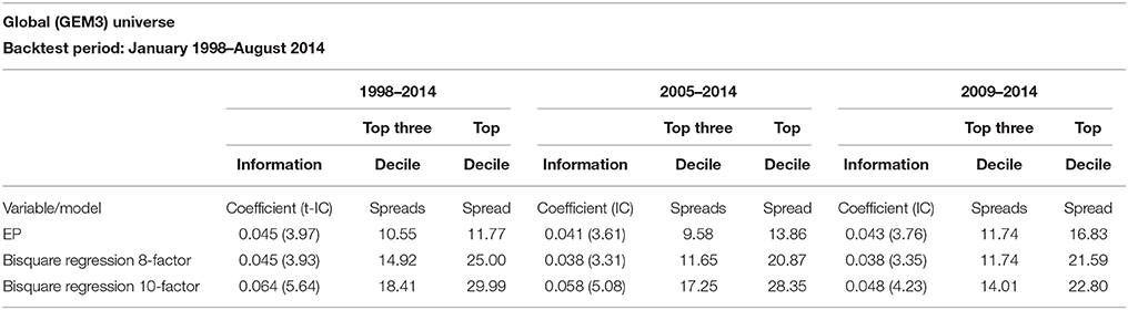
Table 1. Model financial characteristics.

FIGURE 1

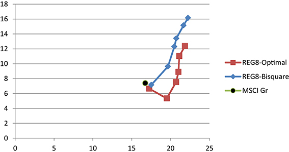
Figure 1. Risk-return portfolios for Beaton-Tukey regressions, 2005–2014.

FIGURE 2

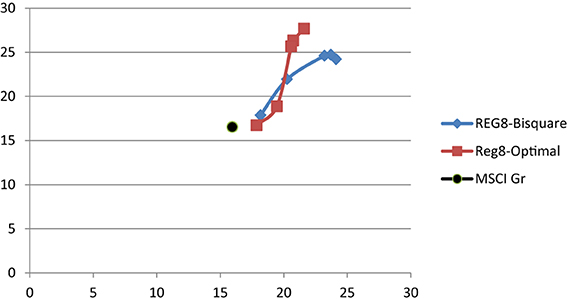
Figure 2. Risk-return portfolios for alternative robust regressions, 2009–2014.

TABLE 2

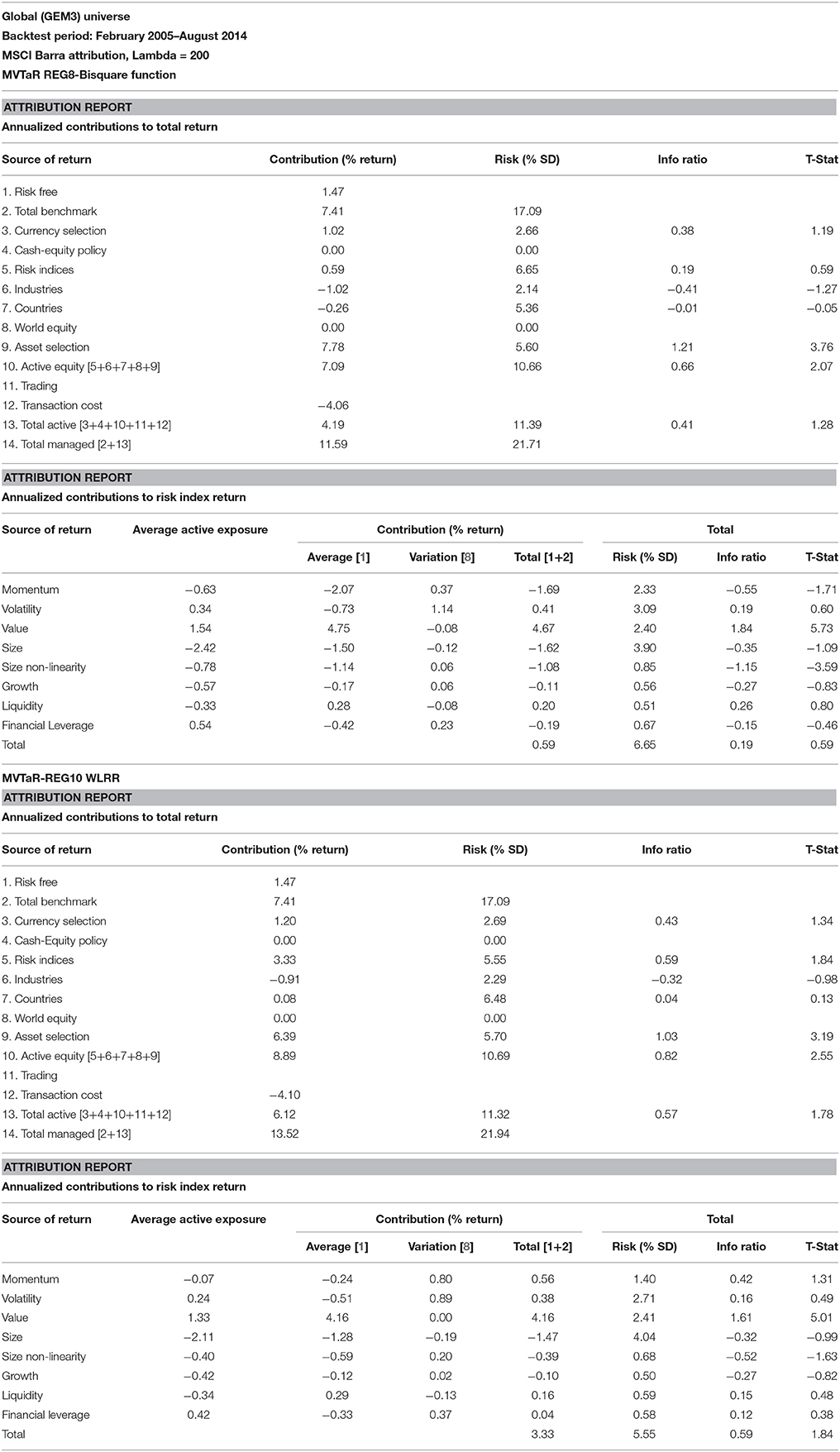
Table 2. Barra attribution of regression-based portfolio.

TABLE 3

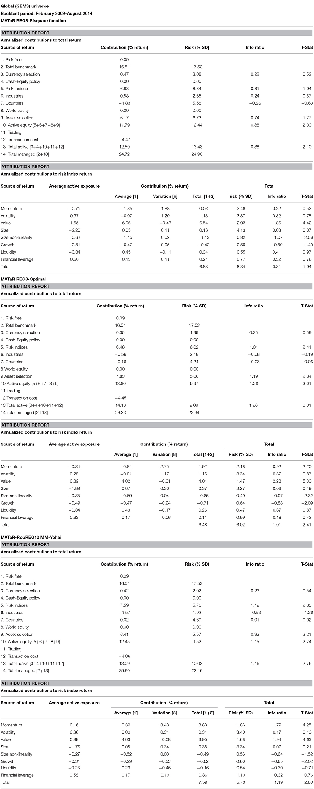
Table 3. Barra attribution of regression-based portfolios.

TABLE 4

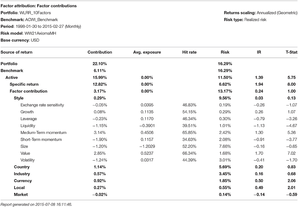
Table 4. Robust regression with the Beaton-Tukey WLRR procedure.

TABLE 5

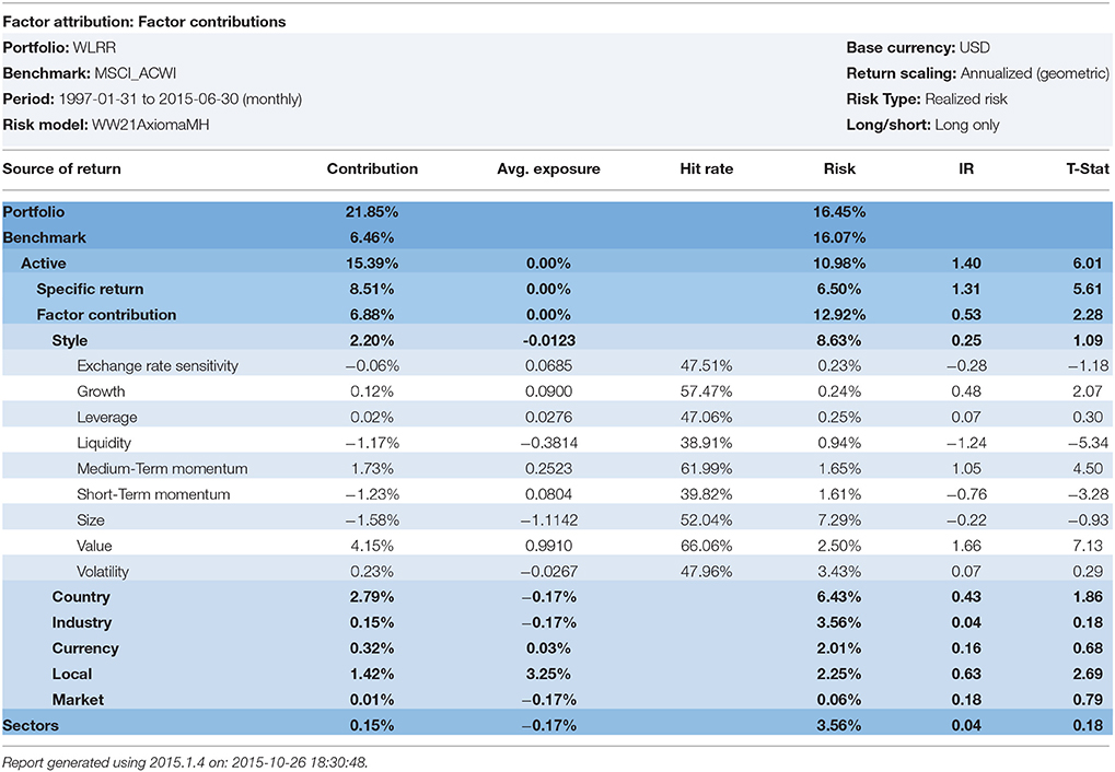
Table 5. Robust regression with WLRR.

TABLE 6

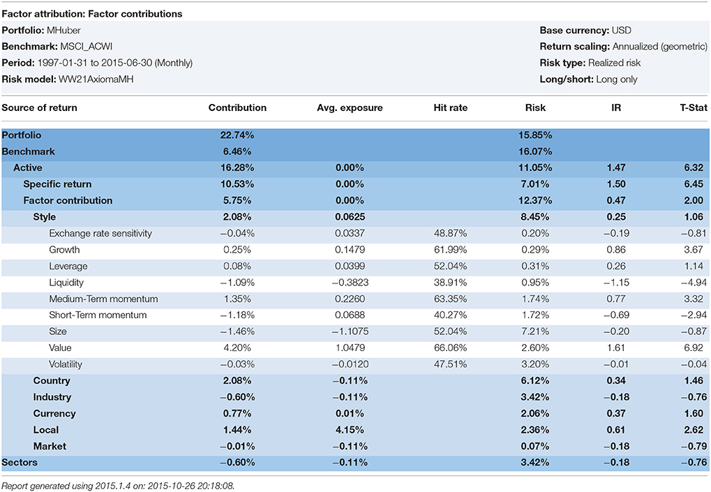
Table 6. Robust regression with Huber.

TABLE 7

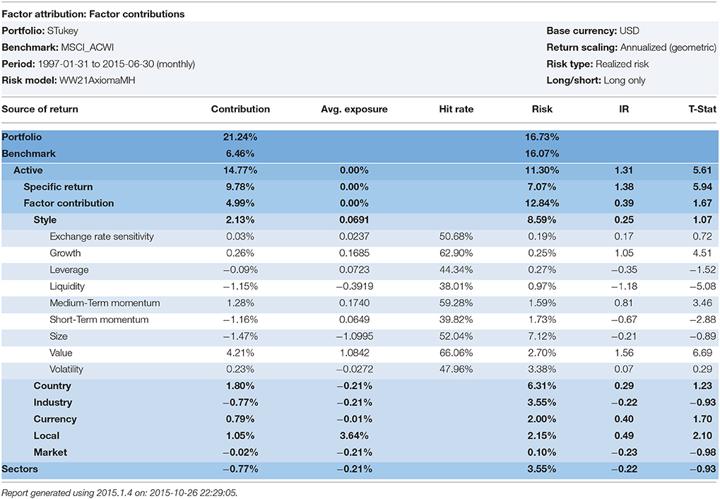
Table 7. Robust regression with the S-procedure of Tukey.

TABLE 8

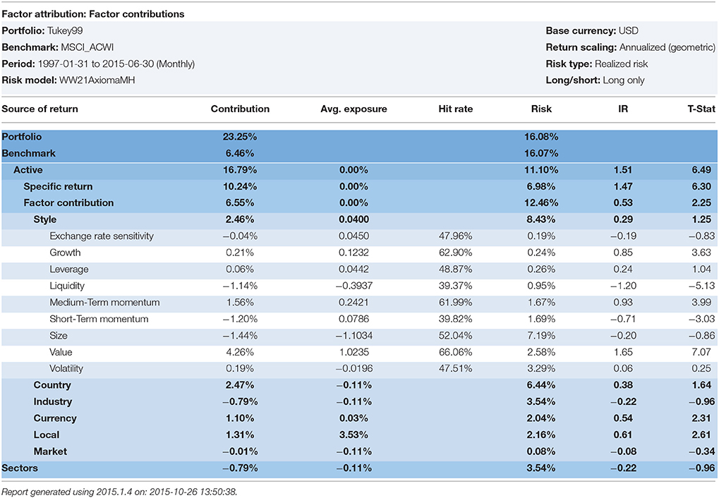
Table 8. Robust regression with MM-procedure with Tukey 99.

TABLE 9

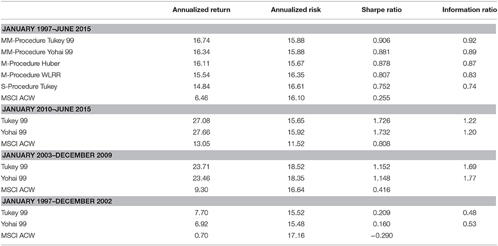
Table 9. Global broad regression BackTest summary results.

Summary and Conclusions

In this analysis, we report evidence confirming the continued relevance of the robust regression models in estimating stock selection models. The Beaton-Tukey Bisquare procedure (approximated with WLRR techniques) has continued to produce statistically significant results in the post-financial crash period. More modern robust regression procedures, such as the Yohai Optimal influence procedure, produce statistically significant stock selection models. All forms of robust regression (M, S, and MM-procedures) outperformance OLS in producing higher portfolio excess returns. The stock selection models are complemented with Markowitz mean-variance optimization models. One must use the most sophisticated of statistical and optimization techniques when markets crash.

Conflict of Interest Statement

The author declares that the research was conducted in the absence of any commercial or financial relationships that could be construed as a potential conflict of interest.

The reviewer, FD, and handling Editor declared their shared affiliation, and the handling Editor states that the process nevertheless met the standards of a fair and objective review. The reviewer, KX, and handling Editor declared their shared affiliation, and the handling Editor states that the process nevertheless met the standards of a fair and objective review.

Acknowledgments

The author acknowledges comments by participants at George Washington University, University of Washington, and the FactSet Research Seminar in Washington, DC. The comments of Doug Martin are greatly appreciated. Abhishek Saxena ran many of the alternative robust regression models reported in Table 9. Any errors remaining are the responsibility of the author.

Footnotes

1. ^The Beaton-Tukey analysis and its weighting of outliers built upon the work of Anscombe [10] and Anscombe and Tukey [11]. The author has worked on robust regression applications for several decades, and enjoyed personal communications with Francis Anscombe on the issue of outliers and estimation in APL.

2. ^Guerard et al. [14] reported highly statistically significant specific returns with CTEF.

3. ^If one deletes observation i in a regression, then one can measure the change in estimated regression coefficients and residuals. The standardized residual concept can be modified such that the reader can calculate a variation on that term to identify influential observations.

4. ^Another distance measure has been suggested by Cook [42], which modifies the studentized residual, to calculate a scaled residual known as the Cook distance measure, CookD.

5. ^The identification of influential data is an important component of regression analysis. The modeler can identify outliers, or influential data, and re-run the ordinary least squares regressions on the re-weighted data, a process referred to as robust (ROB) regression. In ordinary least squares, OLS, all data is equally weighted. The weights are 1.0.

6. ^Doug Martin suggested that the author re-run the robust regressions using the Bisquare and Optimal S-Method models with various efficiency levels (95, 90, and 99%). We ran the analysis from January 1998–February 2015 on an all I/B/E/S forecast global universe that approached 16,000 stocks per month. The Sharpe Ratio is the portfolio excess returns divided by the portfolio standard deviation. The Information Ratio, IR, is the portfolio excess returns divided by the portfolio tracking error. The Yohai Optimal 85% Function produced a Geometric Mean of 18.75%, a Sharpe ratio of 1.251, and an Information ratio of 1.09. The Beaton-Tukey Bisquare produced a Geometric Mean of 19.56%, a Sharpe Ratio of 1.056, and an information Ratio of 1.14. Thus, over a 17-year backtest, the Beaton-Tukey Bisquare produced a higher portfolio standard deviation, leading to a lower Sharpe Ratio, but a higher return relative to its tracking error, leading to a higher Information Ratio, than the Yohai Optimal Function. In Tables 4–8, we report the WLRR, Beaton-Tukey Bisquare S-Method, M-Method with Huber, S-procedure with Tukey and MM-Method with the optimal Tukey 99 of efficiency criteria. The best robust regression procedure is the Tukey 99 efficiency techniques of the 10 factor Model. All models produce highly statistically specific returns, large exposures to the Momentum risk factor, and the Momentum Style factor returns are in the 250–325 basis points range and the t-statistics on Momentum exceed 4.9!

We expanded the 10-factor model to include the 1-month total return reversal, the annualized stock standard deviation, the dividend yield, and relative dividend yield, and a price momentum variable with the market return removed. The proprietary 15-factor model produced Geometric Means of 17.86, 17.23, and 17.39%, respectively, for the S-Method Bisquare weighting procedure for 85, 95, and 99% efficiency levels, whereas the S-Method Yohai Optimal Influence weighting procedure produced corresponding Geometric Means of 17.54, 17.36, and 16.61. The corresponding Morgan Stanley Capital international (MSCI) All Country World Growth benchmark return was 5.53%. Thus, the Bisquare procedure slightly outperformed the Yohai Optimal procedure, but there was no statistical difference in the Geometric Means. The S-Method Bisquare Sharpe Ratios for the 85, 95, and 99% efficiency levels were 1.247, 1.205, and 1.201, whereas the corresponding S-Method Yohai Optimal Sharpe Ratios were 1.217, 1.208, and 1.157. The Bisquare Information Ratios for the 85, 95, and 99% efficiency levels were 0.99, 0.92, and 0.93, whereas the corresponding Optimal Sharpe Ratios were 0.94, 0.92, and 0.88. The corresponding M-method and MM-Method Bisquare IRs were 0.95 and 0.99, for the 15-factor model, respectively. Thus, the MM-method and S-Method Bisquare robust regression models were virtually identical in predictive power and slightly outperformed the M-method Bisquare weighting procedure. The OLS Model for the 15 factors produced a Geometric Mean of 16.97%, a Sharpe Ratio of 1.158, and an IR of 0.96. The best M-Method for the 15-factor model was the Welsch weighting. Virtually all robust regression (M, S, and MM-Methods) techniques outperformed the OLS Model. A summary table, Table 9, contains robust regression results.

References

1. Beaton AE, Tukey JW. The fitting of power series, meaning polynomials, illustrated on bank-spectroscopic data. Technometrics (1974) 16:147–85.

Google Scholar

2. Gunst RF, Webster JT, Mason RL. A comparison of least squares and latent root regression estimators. Technometrics (1976) 18:75–83.

Google Scholar

3. Gunst RF, Mason RL. Regression Analysis and its Application. New York, NY: Marcel Dekker, Inc (1980).

Google Scholar

4. Rousseeuw PJ. Least median of squares regression. J Am Stat Assoc. (1984) 79:871–80.

Google Scholar

5. Rousseeuw PJ, Hubert M. Recent development in PROGRESS. Comput Stat Data Anal. (1996) 21:67–85.

PubMed Abstract

6. Rousseeuw PJ, Leroy AM. Robust Regression and Outlier Detection. New York, NY: John Wiley & Sons (1987).

Google Scholar

7. Rousseeuw PJ, Yohai V. Robust regression by means of S estimators. In: Franke J, Härdle W, Martin RD, editors. Robust and Nonlinear Time Series Analysis, Lecture Notes in Statistics, Vol. 26. New York, NY: Springer-Verlag (1984). pp. 256–274.

8. Yohai VJ, Stahel WA, Zamar RH. A procedure for robust estimation and inference in linear regression. In: Stahel WA, Weisberg SW, editors. Directions in Robust Statistics and Diagnostics, Part II. New York, NY: Springer-Verlag (1991). pp. 365–374.

9. Maronna RA, Martin RD, Yojai VJ. Robust Statistics: Theory and Methods. New York, NY: Wiley (2006).

10. Anscombe FJ. Rejection of outliers. Technometrics (1960) 2:123–47.

Google Scholar

11. Anscombe FJ, Tukey JW. The examination and analysis of residuals. Technometrics (1963) 5:141–59.

Google Scholar

12. Bloch M, Guerard JB Jr, Markowitz HM, Todd P, Xu G-L. A comparison of some aspects of the U.S. and Japanese equity markets. Japan World Econ. (1993) 5:3–26.

Google Scholar

13. Guerard JB Jr, Rachev RT, Shao B. Efficient global portfolios: big data and investment universes. IBM J. Res. Dev. (2013) 57:11. doi: 10.1147/JRD.2013.2272483

CrossRef Full Text | Google Scholar

14. Guerard JB Jr, Markowitz HM, Xu G. Earnings forecasting in a global stock selection model and efficient portfolio construction and management. Int. J. Forecast. (2015) 31:550–60. doi: 10.1016/j.ijforecast.2014.10.003

CrossRef Full Text | Google Scholar

15. Guerard JB Jr, Xu G, Gultekin MN. Investing with momentum: the past, present, and future. J. Invest. (2012) 21:68–80. doi: 10.3905/joi.2012.21.1.068

CrossRef Full Text | Google Scholar

16. Latane HA, Tuttle DL, Jones CP. Security Analysis and Portfolio Management. 2nd Edn. New York, NY: The Roland Press (1975).

17. Markowitz HM. Portfolio Selection: Efficient Diversification of Investment. Cowles Foundation Monograph No.16. New York, NY: John Wiley & Sons (1959).

18. Markowitz HM. Investment in the long run: new evidence for an old rule. J. Finan. (1976) 31:1273–86.

Google Scholar

19. Elton EJ, Gruber MJ, Brown SJ, Goetzman WN. Modern Portfolio Theory and Investment Analysis. 7th Edn. New York, NY: John Wiley & Sons, Inc. (2007).

Google Scholar

20. Graham B, Dodd D. Security Analysis: Principles and Technique. New York, NY: McGraw-Hill Book Company (1934).

21. Williams JB. The Theory of Investment Value. Cambridge, MA: Harvard University Press (1938).

Google Scholar

22. Basu S Investment performance of common stocks in relations to their price earnings ratios: a test of market efficiency. J Finance (1977) 32:663–82.

23. Guerard JB Jr, Stone BK. Composite forecasting of annual earnings. In: Chen A, editor. Research in Finance 10. Greenwich, CT: JAI Press (1992). pp. 205–31.

24. Dimson E. Stock Market Anomalies. Cambridge: Cambridge University Press (1988).

Google Scholar

25. Haugen R, Baker N. Case closed. In: Guerard JB, editor. The Handbook of Portfolio Construction: Contemporary Applications of Markowitz Techniques. New York, NY: Springer (2010). pp. 601–620.

PubMed Abstract

26. Guerard JB Jr. Global earnings forecasting efficiency. In: Kensinger J, editor. Research in Finance 28. Greenwich, CT: JAI Press (2012). pp. 19–48.

27. Guerard, JB Jr, Gultekin M, Stone BK. The role of fundamental data and analysts' earnings breadth, forecasts, and revisions in the creation of efficient portfolios. In: Chen A, editor. Research in Finance 15. Greenwich, CT: JAI Press (1997). pp. 69–92.

28. Fama EF, French KR. Cross-sectional variation in expected stock returns. J Finance (1992) 47:427–65.

29. Fama EF, French KR. Size and the book-to-market factors in earnings and returns. J Finance (1995) 50:131–55.

Google Scholar

30. Fama EF, French KR. Dissecting anomalies. J Finance (2008) 63:1653–678.

Google Scholar

31. Levy RA. Random walk: reality or myths. Financ Anal J. (1967) 23:69–77.

Google Scholar

32. Chan LKC, Jegadeesh N, Lakonishok J. Momentum strategies. J Finance (1996) 51:1681–713.

Google Scholar

33. Conrad J, Kaul G. An anatomy of trading strategies. Rev Financ Stud. (1998) 11:489–519.

Google Scholar

34. Conrad J, Kaul G. Mean reversion in short-horizon expected returns. Rev Financ Stud. (1989) 2:225–40.

Google Scholar

35. Jegadeesh N, Titman S. Returns to buying winners and selling losers: implications for market efficiency. J Finance (1993) 48:65–91.

Google Scholar

36. Sadka R. Momentum and post-earnings-announcement-drift anomalies: the rock of liquidity risk. J Financ Econ. (2006) 80:309–49.

Google Scholar

37. Korajczyk RA, Sadka R. Are momentum profits robust to trading costs? J Finance (2004) 59:1039–82. doi: 10.1111/j.1540-6261.2004.00656.x

CrossRef Full Text | Google Scholar

38. Brush JS, Boles KE. The predictive power in relative strength and CAPM. J Portf Manag. (1983) 9:20–3.

Google Scholar

39. Brush JS. Price momentum: a twenty-year research effort. Columbine Newsletter Special Issue. (2001).

40. Brush JS. A flexible theory of price momentum. J Invest. (2007) 16. doi: 10.3905/joi.2007.681822

CrossRef Full Text | Google Scholar

41. Belsley DA, Kuh E, Welsch RE. Regression Diagnostics: Identifying Influential Data and Sources of Collinearity, Chapter 2. New York, NY: John Wiley & Sons (1980).

Google Scholar

42. Cook RD. Influential observations in linear regression. J Am Statist Associat. (1979) 74:169–74.

Google Scholar

43. Webster JT, Gunst RF, Mason RL. Latent root regression analysis. Technometrics (1974) 16:513–22.

Google Scholar

44. Gunst RF, Mason RL. Some considerations in the evaluation of altrenative prediction equations. Technometrics (1979) 21:55–63.

Google Scholar

45. Mason RL, Gunst RF. Outlier-induced collinearities. Technometrics (1985) 27:401–07.

Google Scholar

46. Carrillo-Gambos O, Gunst RF. Measurement-error-model collinearities. Technometrics (1992) 34:454–64.

PubMed Abstract | Google Scholar

47. Yohai VJ. High breakdown point and high efficiency robust estimates for regression. Ann Stat. (1987) 15:642–56.

Google Scholar

48. Yohai VJ, Zamar RH. Optimal locally robust m- estimate of regression. J Stat Plan Inference (1997) 64:309–23.

Google Scholar

49. Ruppert D. Computing S estimators for regression and multivariate location/dispersion. J Comput Graph Stat. (1992) 1:253–70.

Google Scholar

50. Markowitz H. Mean-Varance Analysis in Portfolio Choice and Capital Markets. London: Basil Blackwell (1987).

Google Scholar

51. Markowitz HM. Portfolio selection. J Finance (1952) 7:77–91.

Google Scholar

52. Markowitz HM. Risk-Return Analysis. New York, NY: McGraw-Hill (2013).

Google Scholar

53. Sharpe WF. Capital asset prices: a theory of market equilibrium under conditions of risk. J Finance (1964) 19:425–42.

Google Scholar

54. Lintner J. The valuation of risk assets and the selection of risk investments in stock portfolios, and capital budgets. Rev Econ Statist. (1965) 47:13–37.

Google Scholar

55. Mossin J. Equilibrium in a capital asset market. Econometrica (1966) 34:768–83.

Google Scholar

56. Mossin J. Theory of Financial Markets. Englewood Cliffs, NJ: Prentice-Hall, Inc (1973).

57. Stone BK. Risk, Return, and Equilibrium: A General Single-Period Theory of Asset Selection and Capital Market Equilibrium. Cambridge, MA: MIT Press (1970).

58. Ross SA. The arbitrage theory of capital asset pricing. J Econ Theory (1976) 13:341–60.

Google Scholar

59. Fama EF, MacBeth JD. Risk, return, and equilibrium: empirical tests. J Pol Econ. (1973) 81:607–36.

Google Scholar

60. Sharpe WF. A simplified model for portfolio analysis. Manag Sci. (1963) 9.

PubMed Abstract | Google Scholar

61. Sharpe WF. A linear programming approximation for the general portfolio analysis problem. J Financ Q Anal. (1971) 6:1263–75.

Google Scholar

62. Rudd A, Rosenberg B. Realistic portfolio optimization. In: Elton E, Gruber M, editors. Portfolio Theory, 25 Years After. Amsterdam: North Holland (1979). pp. 21–46.

63. Stone BK. A linear programming formulation of the general portfolio selection problem. J Financ Q Anal. (1973) 8:621–36.

Google Scholar

64. Black F, Jensen MC, Scholes M. The capital asset pricing model: some empirical tests. In: Jensen M, editor. Studies in the Theory of Capital Markets. New York, NY: Praeger (1972). pp. 79–124.

65. King BF. Market and industry factors in stock price behavior. J Bus. (1966) 39:139–91.

Google Scholar

66. Elton EJ, Gruber MJ. Homogeneous groups and the testing of economic hypothesis. J Financ Q Anal. (1970) 5:581–602.

Google Scholar

67. Reinganum M. The arbitrage pricing theory: some empirical tests. J Finance (1981) 36:313–21.

Google Scholar

68. Rosenberg B. Extra-market components of covariance in security returns. J Financ Q Anal. (1974) 9:263–74.

Google Scholar

69. Rosenberg B, Marathe V. Tests of capital asset pricing hypotheses. In: Levy H, editor. Research in Finance 1. Greenwich, CT: JAI Press (1979). pp. 115–224.

70. Rudd A, Rosenberg B. The ‘Market Model’ in investment management. J Finance (1980) 35:597–607.

Google Scholar

71. Ross SA, Roll R. An empirical investigation of the arbitrage pricing theory. J Finance (1980) 35:1071–103.

Google Scholar

72. Blin JM, Bender S, Guerard JB Jr. Earnings forecasts, revisions and momentum in the estimation of efficient market-neutral japanese and U.S. portfolios. In: Chen A, editor. Research in Finance 15. Greenwich, CT: JAI Press (1997). pp. 93–114.

73. Elton EJ, Gruber MJ, Gültekin MN. Expectations and share prices. Manag Sci. (1981) 27:975–87.

Google Scholar

74. Elton EJ, Gruber MJ. Estimating the dependence structure of share prices—implications for portfolio selection. J Finance (1973) 28:1203–232.

Google Scholar

75. Farrell JL Jr. Analyzing covariance of returns to determine homogeneous stock groupings. J Bus. (1974) 47:186–207.

Google Scholar

76. Stone BK. Systematic interest-rate risk in a two-index model of returns. J Financ Q Anal. (1974) 9:709–21.

Google Scholar

77. Dhrymes PJ, Friend I, Gultekin NB. A critical re-examination of the empirical evidence on the arbitrage pricing theory. J Finance (1984) 39:323–46.

Google Scholar

78. Menchero J, Morozov A, Shepard P. Global equity modeling. In: Guerard JB, editor. The Handbook of Portfolio Construction: Contemporary Applications of Markowitz Techniques. New York, NY: Springer (2010). pp. 439–80.

79. Farrell JL Jr. Portfolio Management: Theory and Applications. New York, NY: McGraw-Hill; Irwin (1997).

80. Haugen RA. Modern Investment Theory. 5th ed. Prentice Hall (2001).

Google Scholar

81. Conner G, Korajczyk RA. Factor models in portfolio and asset pricing theory. In: Guerard J, editor. The Handbook of Portfolio Construction: Contemporary Applications of Markowitz Techniques. New York, NY: Springer (2010). pp. 401–418.

PubMed Abstract

82. Connor G, Goldberg L, Korajczyk RA. Portfolio Risk Analysis. Princeton, NJ: Princeton University Press (2010).

Google Scholar

83. Grinold R, Kahn R. Active Portfolio Management. New York, NY: McGraw-Hill; Irwin (1999).

Google Scholar

84. Markowitz HM, Xu GL. Data mining corrections. J Portf Manag. (1994) 21:60–9.

Google Scholar