A mathematical analysis of the corruption dynamics model with optimal control strategy

1 Introduction

Corruption is an ancient and worldwide problem that destroys the economic development associated with all companies and human associations [1]. Corruption is an unlawful activity carried out for personal benefit, and the benefit of corruption is obtained by misuse of power by public or private officeholders [2]. Corruption is considered one of the frightening components for sustainable economic growth, moral values, and justice because it disturbs social life and the rule of law [3, 4]. Corruption affects the development of many countries around the world by reducing the national economy and the internal peace and security [5, 6]. Corruption is the major cause of poverty around the world, especially in Africa, and it hinders economic development, undermines democracy, and damages social justice and the rule of law [7, 8]. In Ethiopia, corruption affects political systems such as democratic power sharing, accountable and transparent institutions, and procedures. Furthermore, it is one of the causes of instability and conflict as observed in the present situations [9, 10].

The spread of corruption can be understood just as it is similar to the spread of diseases from one infected person to another susceptible individual in society, which means a non-corrupt individual gets infected with a high probability if the number of corrupt individuals in the social neighborhood exceeds a certain threshold value; in the case of mean field dependence, an individual can get corrupted because there is a high prevalence in society [10]. Introducing strong measures against the corruption is a very difficult task, since the nature of corruption practices is very secretive and illicit. However, within a society or country, it is possible to educate people and change their attitude against corruption [11]. However, it requires a thorough understanding of corruption processes to develop intervention strategies to prevent and mitigate corruption practices [12].

In epidemiology, mathematical modeling plays an important role. It is an effective tool to understand and describe the dynamics and transmission of infectious diseases [13]. Therefore, several authors, including the study mentioned in the references [14–19], have developed and analyzed mathematical models that represent the approach of corruption dynamics as a disease transmission model to evaluate the effects of corruption on national development. Furthermore, several researchers have developed mathematical models to represent corruption dynamics following the approaches adopted in epidemiology. Let us now review some of such models here.

Hathroubi [20] explained the dynamics of corruption in a closed population using the epidemiological SIR (Susceptible, Infected and Removed) model. He has determined the threshold for the transmission of corruption based on the size of the honest population. However, he did not perform stability analyses of both corruption-free and endemic equilibrium points.

Abdulrahman [11] proposed a deterministic mathematical model with constant recruitment rates and standard incidence rates for the transmission dynamics of corruption as a disease. He extended the study by Hathroubi [20] and formulated a non-linear mathematical model for describing the corruption transmission. Furthermore, he divided the total population into four compartments depending on their status of corruption: Susceptible S(t), Corrupt C (t), Jailed J (t), and Honest H (t). Employing the Jacobian matrix method and Lyapunov function approach, he examined and analyzed the stability of both corruption-free and endemic equilibrium points, respectively. Numerical simulations were also carried out and confirmed the analytical results. Additionally, these results revealed that corruption can only be reduced to a manageable level but cannot be completely eliminated.

Legesse and Shiferaw [10] proposed a mathematical model for corruption by considering awareness created by anticorruption and counseling in jail. They divided the total population into four compartments, namely, Susceptible S(t), Corrupt C (t), Jailed J (t), and Honest H (t) individuals and proved that the model is both epidemiological and mathematically well-posed. In their model, stability analyses of both corruption-free and endemic equilibrium were carried out. In addition, the simulation result shows agreement with the analytical result. However, they did not design optimal control strategies to minimize the spread of corruption. Alemneh [21] developed a mathematical model of corruption dynamics by dividing the total population into five compartments; such as Susceptible S(t), Exposed to corruption E (t), Corrupt C (t), Recovered R (t), and Honest H (t) individuals. He analyzed both the local and global asymptotic stability of the corruption-free and endemic equilibrium. He extended the model to optimal control and explored its numerical simulation. He also suggested that an integrated control strategy should be taken to combat corruption.

Despite many researchers conducting mathematical modeling to control corruption transmission, this problem remains present. The present study developed a mathematical model that represents corruption dynamics by modifying the study conducted in Alemneh [21] to understand better control measures of corruption. This model is further extended to include optimal control strategy with the following two time-dependent control measures: (i) mass education of the susceptible individuals and (ii) law enforcement on the corrupted individuals. Therefore, the study is organized as follows. Section 2 explains the formulation and description of the model that represents corruption dynamics. Section 3 represents basic properties and model analysis including positivity, invariant region, existence of equilibrium, and stability of the model. In Section 4, the optimal control strategy is presented. In Section 5, the numerical simulation of the model is also analyzed. The conclusion is presented in Section 6.

2 Formulation and description of the model

The present corruption dynamics model is a modification of the existing model done by Alemneh [21] by dividing the total population N(t) into six compartments based on their corruption status. These are susceptible individuals S(t), exposed individuals E(t), corrupted individuals C(t), jailed individuals J(t), recovered individuals R(t), and honest individuals H(t). Therefore, the total population is given as N(t) = S(t)+E(t)+C(t)+R(t)+J(t)+H(t) and the six compartments are further described as follows:

(i) Susceptible individuals S(t): This compartment contains individuals who have not been involved so far in any type of corruption. In addition, it contains individuals who are already involved in corruption activities but completed the jail and thus became susceptible. People enter into this compartment naturally by birth and from the jailed compartment after finishing their jail term. However, some of them can leave this compartment and move to exposed and honest compartments.

(ii) Exposed individuals E(t): This compartment contains individuals who are already exposed to corruption. Although these people are already corrupted, they cannot influence or convert any susceptible individual into corrupted. People will enter from a susceptible compartment only. However, some of them can leave this compartment and move to corrupted and honest compartments.

(iii) Corrupted individuals C(t): These people are capable of influencing or converting any susceptible individual to be corrupted. In other words, these individuals can encourage and facilitate susceptible individuals to participate in corruption activities. This compartment contains individuals who are generated only from the exposed compartment. However, some of them can leave this compartment and move to jailed and recovered compartments.

(iv) Jailed individuals J(t): These are the people who were already engaged in corruption activities and caught. As a result, these people are imprisoned for a specified period of time, and hence they are now in jail. People will enter into this from corrupted and recovered compartments. Similarly, after they finish their imprisonment period, people can move either to the susceptible or honest compartment as they wish.

(v) Recovered individuals R(t): These are the people who had earlier participated in corruption activities but later left voluntarily. However, these individuals will move to the jailed compartment if they are proven to be involved in corrupted activities. Otherwise, they will move to the honest compartment.

(vi) Honest individuals H(t): These are the people who do not participate in any corruptive activity and have no negative impact on their country's development. People in susceptible, exposed, recovered, and jailed compartments can enter this compartment.

We now describe the flow rates of individuals from one compartment to the others as follows:

Flow of susceptible individuals S(t): Individuals are recruited with a constant birth rate Π. Furthermore, after release from jail, individuals will join susceptible individuals at a rate (1 − φ)θ. Similarly, whenever susceptible individuals contact corrupted people, they become exposed at a rate ρβ, while others can join the honest compartment at a rate γ.

Flow of exposed individuals E(t): When influenced by corrupted people, susceptible individuals will be exposed to corruption and will enter this compartment at a rate of ρβ. However, individuals of the exposed compartment will go to the corrupt compartment at the rate of ωφ and to the honest compartment at a rate of (1 − ω)ϕ.

Flow of corrupted individuals C(t): Individuals from the exposed compartment will move into the corruption compartment at a rate of ωφ. However, people will move out of the corrupted compartment to the jailed compartment at a rate of τ and to the recovered compartment at a rate of δ, respectively.

Flow of recovered individuals R(t): Upon leaving corruptive activities, individuals in the corrupted compartment will move to the recovery compartment at a rate of δ. However, they move to jailed compartments at a rate of ηα and honest compartment at a rate of (1 − η)α, respectively. Finally, we assumed the natural death rate μ in all compartments.

Depending on the assumptions and descriptions of the parameters and variables, the flow diagram of the compartmental model is shown in Figure 1.

Figure 1

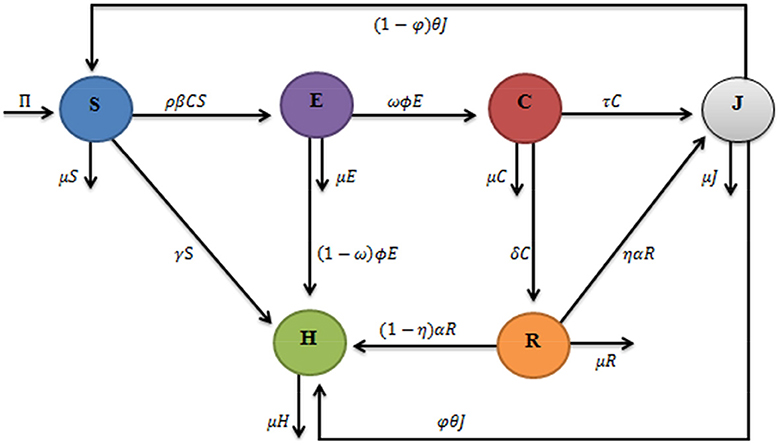
Figure 1. Compartmental flow diagram of corruption model.

Based on the flow diagram in Figure 1, we obtained the system of non-linear ordinary differential equations that represent the corruption dynamics as follows:

$\begin{array}{ll}\{\begin{array}{c}\begin{array}{c}\frac{dS}{dt}=\Pi +(1-\phi )\theta J-\rho \beta CS-(\gamma +\mu )S,\\ \frac{dE}{dt}=\rho \beta CS-(\varphi +\mu )E,\\ \frac{dC}{dt}=\omega \varphi E-(\delta +\tau +\mu )C,\end{array}\\ \begin{array}{c}\frac{dR}{dt}=\delta C-(\alpha +\mu )R,\\ \frac{dJ}{dt}=\tau C+\eta \alpha R-(\theta +\mu )J,\\ \frac{dH}{dt}=\gamma S+(1-\omega )\phi E+(1-\eta )\alpha R+\phi \theta J-\mu H,\end{array}\end{array}& (1)\end{array}$

With the following initial condition

$\begin{array}{l}S(0)>0,E(0)\ge 0,C(0)\ge 0,R(0)\ge 0,\\ J(0)\ge 0,H(0)\ge 0.& (2)\end{array}$

Descriptions of the parameters in the model are presented in Table 1.

Table 1

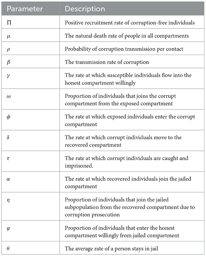
Table 1. Description of the parameters in the model.

Descriptions of the variables in the model are presented in Table 2.

Table 2

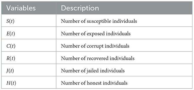
Table 2. Description of the variables in the model.

3 Model analysis

In this section, we investigate the positive solution of the system (1), its boundedness, and positive invariance. In addition, the basic reproduction number, the existence of equilibrium, and the stability of the model are explored and analyzed.

3.1 Positivity solution of the model

Examining the positivity of the solution of dynamical systems is an imaginary approach to ensure the non-negativity of the solution [22]. This investigation has been carried out in several works on mathematical and epidemiological modeling. Therefore, to show that the presented model (1) is epidemiologically and mathematically meaningful, we consider the state variables of the model to be non-negative for all given time t > 0. Thus, we state the following result.

Theorem 1 The initial population S (0) ≥ 0, E (0) ≥ 0, C (0) ≥ 0, R (0) ≥ 0, J (0) ≥ 0 and H (0) ≥ 0 such that the solutions of the system (1) S (t), E (t), C (t), R (t), J (t), H (t) are non-negative for all t ≥ 0.

Proof: Assume that all state variables are continuous. Then, from the third equations system of (1) which is given as follows:

$\begin{array}{c}\frac{dC}{dt}=\omega \varphi E-(\delta +\tau +\mu )C,\\ \frac{dC}{C}=\left[\frac{\omega \phi E}{C}-(\delta +\tau +\mu )\right]dt,\end{array}$

$C(t)=A_1{e}^{\int \left[\frac{\omega \phi E}{C}-(\delta +\tau +\mu )\right]dt}$. Here, A₁ is the integral constant.

By using the initial condition of Equation (2) that is C(0) ≥ 0, we obtain $C(0)=A_1{e}^{{\left\{\int \left[\frac{\omega \phi E}{C}-(\delta +\tau +\mu )\right]dt\right\}}_{t=0}}.$ Eliminating the integral constant A₁ the particular solution is obtained as follows:

$\begin{array}{l}C(t)=C(0)e^{\left\{\int \left[\frac{\omega \phi E}{C}-(\delta +\tau +\mu )\right]dt-{\left\{\int \left[\frac{\omega \phi E}{C}-(\delta +\tau +\mu )\right]dt\right\}}_{t=0}\right\}}\end{array}$

By using the initial condition C(0) ≥ 0, every exponential function is a positive quantity regardless of the sign of the exponent, i.e., e^x ≥ 0.

Hence, $C(t)=C(0)e^{\left\{\int \left[\frac{\omega \phi E}{C}-(\delta +\tau +\mu )\right]dt-{\left\{\int \left[\frac{\omega \phi E}{C}-(\delta +\tau +\mu )\right]dt\right\}}_{t=0}\right\}}$ ≥ 0, thus we conclude that C(t) is positive.

Similarly, we have:

$\begin{array}{ll}\begin{array}{c}R(t)\ge R(0)e^{-(\alpha +\mu )t}\ge 0,\\ J(t)\ge J(0)e^{-(\theta +\mu )t}\ge 0,\\ S(t)\ge S(0)e^{\left\{\int \left[-(\rho \beta C+\gamma +\mu )\right]dt-{\left\{\int \left[-(\rho \beta C+\gamma +\mu )\right]dt\right\}}_{t=0}\right\}}\ge 0,\\ E(t)\ge E(0)e^{-(\varphi +\mu )t}\ge 0,\\ H(t)\ge H(0)e^{-\mu t}\ge 0.\end{array}& (3)\end{array}$

Hence, from Equation (3) we concluded that the solutions S (t), E (t), C (t), R (t), J (t), and H (t) of the system (1) are positive for all t ≥ 0. This result is very essential because the state variables denote human beings and cannot be represented by negative values.

3.2 Invariant region

Furthermore, to show that the formulated corruption model is mathematically and epidemiologically meaningful, we consider the analysis of the system (1) in the feasible region $\Omega \subseteq R_{+}^6$ such that

$\begin{array}{l}\Omega =\{(S,E,C,R,J,H)\in R_{+}^6:0\le S+E+C\\ +R+J+H=N(t)\le \frac{\Pi }{\mu }\}.& (4)\end{array}$

Theorem 2 The feasible solutions of system (1) all entered and bounded in the region Ω.

Proof: The invariance region Ω of Equation (4) is obtained by adding all equations in system (1), and the simplified equation is written as follows:

$\begin{array}{ll}\frac{dN}{dt}=\Pi -\mu N.& (5)\end{array}$

By rearranging and multiplying both sides of Equation (5) by integrating factors, and after some simplification, we obtained the following:

$\begin{array}{ll}N\left(t\right)=\left(\frac{\Pi }{\mu }\right)+\left[N\left(0\right)-\left(\frac{\Pi }{\mu }\right)\right]e^{-\mu t}.& (6)\end{array}$

From Equation (6), we find $\underset{t\to \infty }{lim}N(t)\le \frac{\Pi }{\mu }$. This indicates that the total population N(t) takes off from the initial value N(0) at the beginning and ends up with the bounded value $\frac{\Pi }{\mu }$ as time tends to infinity. Thus, it can be concluded that N(t) is bounded, i.e., $0\le N(t)\le \frac{\Pi }{\mu }$. Hence, the solution set of the system (1) enters and remains in the feasible region Ω, where the model is said to be mathematically and epidemiologically well-posed [23, 24].

3.3 The point of corruption-free equilibrium of the model

To find the corruption-free equilibrium point ${\mathcal{P}}_0=(S^0,E^0,C^0,R^0,J^0,H^0)$ in the model, we equate the right-hand sides of the system of Equation (1) to zero and take the corruption-free compartment E = C = 0. This yields R = 0 and J = 0. Thus, the corruption-free equilibrium point of system (1) is written as follows:

$\begin{array}{ll}{\mathcal{P}}_0=\left(\begin{array}{cccccc}\frac{\Pi }{(\gamma +\mu )}& 0,& 0,& 0,& 0,& \frac{\gamma \Pi }{\mu (\gamma +\mu )}\end{array}\right).& (7)\end{array}$

3.4 Basic reproduction number

The basic reproductive number R₀ is the average number of new corrupts formed after the susceptible and corrupt population contact each other [25–27]. Now, as explained in Theorem 2 in [26], we used the basic reproduction number to determine the spread of corruption. Thus, for R₀ < 1, the corruption will not be able to spread in the population, but if R₀ > 1, corruption will be able to spread in the population, which allows control measures of corruption. In the following result, we compute the basic reproduction number using the next-generation matrix technique described by the study mentioned in the reference [28]. In particular, using the notation in the study mentioned in the reference [28], the Jacobian matrix of the new infection terms (F), and the transfer terms (V), we compute the basic reproduction number. Thus, the matrix of new corrupt terms and transition terms is obtained from the corrupt compartments (i.e., E, C, R, and J) at corruption-free equilibrium and given as follows:

$\begin{array}{ll}\begin{array}{c}\frac{dE}{dt}=\rho \beta CS-(\varphi +\mu )E,\\ \frac{dC}{dt}=\omega \varphi E-(\delta +\tau +\mu )C,\\ \frac{dR}{dt}=\delta C-(\alpha +\mu )R,\\ \frac{dJ}{dt}=\tau C+\eta \alpha R-(\theta +\mu )J.\end{array}& (8)\end{array}$

From system Equation (8), we obtained the general transition matrix f_i and the transmission matrix${\mathcal{V}}_i$ as follows:

$\begin{array}{l}{f}_i=\left[\begin{array}{c}\rho \beta CS\\ 0\\ 0\\ 0\end{array}\right],\text{ and }{\mathcal{V}}_i=\left[\begin{array}{c}(\varphi +\mu )E\\ (\delta +\tau +\mu )C-\omega \varphi E\\ (\alpha +\mu )R-\delta C\\ (\theta +\mu )J-\tau C-\eta \alpha R\end{array}\right],\end{array}$

Where the matrix ${\mathcal{V}}_i(x)$ is defined as ${\mathcal{V}}_i(x)={\mathcal{V}}_i^{-}(x)-{\mathcal{V}}_i^{+}(x)$ with ${\mathcal{V}}_i^{-}(x)=\left[\begin{array}{c}(\varphi +\mu )E\\ (\delta +\tau +\mu )C\\ (\alpha +\mu )R\\ (\theta +\mu )J\end{array}\right],{\mathcal{V}}_i^{+}(x)=\left[\begin{array}{c}0\\ \omega \phi EJ\\ \delta C\\ \tau C+\eta \alpha R\end{array}\right],$

The Jacobian matrices at the corruption-free equilibrium point $({\mathcal{P}}_0)$ yield the matrices F and V, respectively, where

$\begin{array}{r}F=\left[\frac{\partial f_c}{\partial x_j}({\mathcal{P}}_0)\right]=\left|\begin{array}{cccc}0& \frac{\rho \beta \Pi }{(\gamma +\mu )}& 0& 0\\ 0& 0& 0& 0\\ 0& 0& 0& 0\\ 0& 0& 0& 0\end{array}\right|,\\ V=\left[\frac{\partial {\mathcal{V}}_c}{\partial x_j}({\mathcal{P}}_0)\right]=\left(\begin{array}{cccc}(\varphi +\mu )& 0& 0& 0\\ -\omega \varphi & (\delta +\tau +\mu )& 0& 0\\ 0& -\delta & (\alpha +\mu )& 0\\ 0& -\tau & -\eta \alpha & (\theta +\mu )\end{array}\right),\\ F{V}^{-1}=\left[\begin{array}{cccc}\frac{\rho \beta \Pi \omega \varphi }{(\delta +\tau +\mu )(\gamma +\mu )(\varphi +\mu )}& \frac{\rho \beta \Pi }{(\gamma +\mu )(\delta +\tau +\mu )}& 0& 0\\ 0& 0& 0& 0\\ 0& 0& 0& 0\\ 0& 0& 0& 0\end{array}\right],\end{array}$

Thus, the basic reproduction number R₀ of the corruption model is the largest eigenvalue of the next generation matrix. Therefore,

$\begin{array}{ll}{R}_0=\frac{\rho \beta \Pi \omega \varphi }{(\delta +\tau +\mu )(\gamma +\mu )(\varphi +\mu )}.& (9)\end{array}$

3.5 Stability of corruption-free equilibrium point

Theorem 3 The corruption-free equilibrium point $({\mathcal{P}}_0)$ of the system (1) is locally asymptotically stable in Ω if R₀ < 1.

Proof: We used the Jacobian stability techniques on system (1) to determine the corruption-free equilibrium point $({\mathcal{P}}_0)$ as follows:

$\begin{array}{c}J({\mathcal{P}}_0)\\ =\left[\begin{array}{cccccc}-(\gamma +\mu )& 0& -\frac{\rho \beta \Pi }{(\gamma +\mu )}& 0& (1-\phi )\theta & 0\\ 0& -(\varphi +\mu )& \frac{\rho \beta \Pi }{(\gamma +\mu )}& 0& 0& 0\\ 0& \omega \phi & -(\delta +\tau +\mu )& 0& 0& 0\\ 0& 0& \delta & -(\alpha +\mu )& 0& 0\\ 0& 0& \tau & \eta \alpha & -(\theta +\mu )& 0\\ \gamma & (1-\omega )\varphi & 0& (1-\eta )\alpha & \phi \theta & -\mu \end{array}\right].& (10)\end{array}$

From the Jacobian matrix of system Equation (10), we obtained the characteristic polynomial equation of the following form:

$\begin{array}{c}(-\mu -\lambda )(-(\gamma +\mu )-\lambda )(-(\theta +\mu )-\lambda )(-(\alpha +\mu )-\lambda )\\ \left[{\lambda }^2+k_1\lambda +k_2\right]=0.& (11)\end{array}$

where

$\begin{array}{ll}\begin{array}{c}{k}_1=\varphi +\delta +\tau +2\mu ,\\ k_2=(\delta +\tau +\mu )(\varphi +\mu )-\frac{\rho \beta \Pi \omega \phi }{(\gamma +\mu )}.\end{array}& (12)\end{array}$

Hence, from Equation (11), we have eigenvalues,

$\begin{array}{c}{\lambda }_1=-\mu <0,{\lambda }_2=-(\gamma +\mu )<0,\\ {\lambda }_3=-(\theta +\mu )<0,{\lambda }_4=-(\alpha +\mu )<0.& (13)\end{array}$

The two lasting eigenvalues are solutions of the quadratic equation ${\lambda }^2+k_1\lambda +k_2=0$. After substituting the value of k₁ and k₂ from the system of Equation (12), we obtain the following:

$\begin{array}{c}{\lambda }^2+(\varphi +\delta +\tau +2\mu )\lambda +(\delta +\tau +\mu )(\varphi +\mu )\\ -\frac{\rho \beta \Pi \omega \phi }{(\gamma +\mu )}=0.& (14)\end{array}$

Using the Routh–Hurwitz criterion principle [29], Equation (14) has negative real eigenvalues if and only if k₁ > 0, and k₂ > 0. As we observe, k₁ = (ϕ + δ + τ + 2μ) > 0 because it is the sum of positive parameters in the model. In addition, the value of k₂ is explained as follows:

$\begin{array}{l}{k}_2=(\delta +\tau +\mu )(\varphi +\mu )-\frac{\rho \beta \Pi \omega \phi }{(\gamma +\mu )}\\ =(\delta +\tau +\mu )(\varphi +\mu )(1-R_0).& (15)\end{array}$

From Equation (15), the value of k₂ > 0 if and only if R₀ < 1 and hence, all the determinants of the eigenvalues of Equation (11) will have negative real eigenvalues. Therefore, the corruption-free equilibrium point $({\mathcal{P}}_0)$ is locally asymptotically stable if R₀ < 1. The epidemiological implication of Theorem 3 is that corruption can be reduced in the population based on the initial sizes of the sub-populations.

Theorem 4 The corruption-free equilibrium point $({\mathcal{P}}_0)$ of the system (1) is globally asymptotically stable in Ω if R₀ < 1.

Proof : Let us consider the following Lyapunov function for the model (1)

$\begin{array}{ll}F=r_{1}E+r_{2}C.& (16)\end{array}$

Differentiating the Lyapunov function of Equation (16) with respect to time t, we have:

$\begin{array}{ll}\frac{dF}{dt}=r_1\frac{dE}{dt}+r_2\frac{dC}{dt}.& (17)\end{array}$

By substituting the value of $\frac{dE}{dt}$ and $\frac{dC}{dt}$ from the system of Equation (1) into Equation (17), we obtain the following:

$\begin{array}{r}\frac{dF}{dt}=r_1\left[(\rho \beta \Pi CS-(\varphi +\mu )E\right]+r_2\left[(\omega \varphi E-\left(\delta +\tau +\mu \right)C\right],\\ =r_1(\rho \beta \Pi CS-r_2\left(\delta +\tau +\mu \right)C-r_1(\varphi +\mu )E+r_2\omega \phi E,\\ =\frac{\omega \phi }{\left(\varphi +\mu \right)}(\rho \beta \Pi CS-\left(\delta +\tau +\mu \right)C.\end{array}$

By taking the value of $r_1=\frac{\omega \phi }{(\varphi +\mu )}{r}_2$ and r₂ = 1, since S ≤ S⁰ we get the following:

$\begin{array}{r}\frac{dF}{dt}\le \left[\frac{\rho \beta \Pi \omega \phi }{(\varphi +\mu )(\gamma +\mu )}-(\delta +\tau +\mu )\right]C,\\ =\left[\left(\frac{\rho \beta \Pi \omega \phi }{(\delta +\tau +\mu )(\varphi +\mu )(\gamma +\mu )}-1\right)(\delta +\tau +\mu )\right]C,\\ =\left[(R_0-1)(\delta +\tau +\mu )\right]C.& (18)\end{array}$

Hence, from Equation (18) we obtained $\frac{dF}{dt}<0$ for R₀ < 1 and $\frac{dF}{dt}=0$ when C = 0. Therefore, using LaSalle [30], corruption-free equilibrium point is globally asymptotically stable for R₀ < 1.

3.6 Corruption endemic equilibrium point

The corruption endemic equilibrium $({\mathcal{P}}_1)$ is the existence of corruption in a population and denoted by $({\mathcal{P}}_1)=(S^{*},E^{*},C^{*},R^{*},J^{*},H^{*})$. It is obtained by setting the system of Equation (1) to zero as explained in the study mentioned in the reference [31].

$\begin{array}{ll}\frac{dS}{dt}=\frac{dE}{dt}=\frac{dC}{dt}=\frac{dR}{dt}=\frac{dJ}{dt}=\frac{dH}{dt}=0.& (19)\end{array}$

Hence, the corruption-existent equilibrium point was derived as follows:

$\begin{array}{ll}\{\begin{array}{c}{S}^{*}=\frac{\Pi +(1-\phi )\theta J^{*}}{\rho \beta C^{*}+(\gamma +\mu )},\\ E^{*}=\frac{\rho \beta C^{*}{S}^{*}}{(\varphi +\mu )},\\ R^{*}=\frac{\delta C^{*}}{(\alpha +\mu )},\\ J^{*}=\frac{\delta C^{*}+\eta \alpha R^{*}}{(\theta +\mu )},\\ H^{*}=\frac{\gamma S^{*}+(1-\omega )\varphi E^{*}+{(1-\eta )\alpha R}^{*}+\phi \theta J^{*}}{\mu }.\end{array}& (20)\end{array}$

After some simplification of Equation (20), the value of C^* was obtained from the equation three of system (1) as follows:

$\begin{array}{ll}{C}^{*}=\frac{k_1(R_0-1)}{\rho \beta (k_2+k_3)}.& (21)\end{array}$

where

$\begin{array}{l}\begin{array}{c}{k}_1=(\theta +\mu )(\alpha +\mu )(\delta +\tau +\mu )(\varphi +\mu )(\gamma +\mu ),\\ k_2=(\theta +\mu )(\alpha +\mu )(\delta +\tau +\mu )(\varphi +\mu ),\\ k_3=(\omega \theta \tau \alpha +\omega \theta \tau \mu +\omega \theta \eta \alpha \delta )(1-\varphi ).\end{array}\end{array}$

Recalling that all the parameters of the model are positive. Hence, if R₀ > 1, from Equation (21), we obtain the value of $C^{*}=\frac{k_1(R_0-1)}{\rho \beta (k_2+k_3)}>0$. This indicates the existence of corruption in the entire population and the presence of corruption-endemic equilibrium point.

3.7 Stability of corruption-endemic equilibrium point

Theorem 5 The corruption endemic equilibrium point $({\mathcal{P}}_1)$ of the system (1) is globally asymptotically stable in Ω if R₀ > 1.

Proof: We used the following Lyapunov function as explained in the study mentioned in the reference [32, 33], to prove the global stability of the endemic equilibrium point.

$\begin{array}{ll}L=\frac{1}{2}{\left[B_1+B_2+B_3+B_4+B_5+B_6\right]}^2.& (22)\end{array}$

where

$\begin{array}{l}{B}_1=(S-S^{*}),B_2=(E-E^{*}),\\ B_3=(C-C^{*}),B_4=(R-R^{*}),\\ B_5=(J-J^{*}),B_6=(H-H^{*}).\end{array}$

By differentiating Equation (22) with respect to time (t), we obtain the following result:

$\begin{array}{r}\frac{dL}{dt}=\left(\begin{array}{c}\left[\left(S-S^{*}\right)+\left(E-E^{*}\right)+\left(C-C^{*}\right)+\left(R-R^{*}\right)+\left(J-J^{*}\right)+\left(H-H^{*}\right)\right]\\ \left[\frac{dS}{dt}+\frac{dE}{dt}+\frac{dC}{dt}+\frac{dR}{dt}+\frac{dJ}{dt}+\frac{dH}{dt}\right]\end{array}\right),\\ \frac{dL}{dt}=\left[\left(S-S^{{}^{**}}\right)+\left(E-E^{{}^{**}}\right)+\left(C-C^{{}^{**}}\right)+\left(R-R^{{}^{**}}\right)+\left(J-J^{{}^{**}}\right)+\left(H-H^{*}\right)\right]\frac{dN}{dt}.& (23)\end{array}$

By substituting Equation (4) into Equation (23) and simplifying, we get the following expression:

$\begin{array}{c}\frac{dL}{dt}=[\left(S+E+C+R+J+H\right)\\ -\left(S^{\ast }+E^{\ast }+C^{\ast }+R^{\ast }+J^{\ast }+H^{\ast }\right)]\left[\Pi -\mu N\right].\\ \frac{dL}{dt}\le \left[N-\frac{\Pi }{\mu }\right]\left[\Pi -\mu N\right].& (24)\end{array}$

By simplifying Equation (24), we achieve the following result:

$\begin{array}{ll}\frac{dL}{dt}\le -\frac{1}{\mu }{\left[\Pi -\mu N\right]}^2.& (25)\end{array}$

Thus, Equation (25) shows that $\frac{dL}{dt}<0$ and also $\frac{dL}{dt}=0,$ if and only if S = S^*, E = E^*, C = C^*, R = R^*, J = J^*, and H = H^*. Then, the largest invariant set of the system (1) on the set $(S,E,C,R,J,H)\in \Omega \subset R_{+}^6:\frac{dL}{dt}\le 0$ is the endemic equilibrium point. Using the LaSalle invariance principle [30], we indicated that the endemic equilibrium point $({\mathcal{P}}_1)$ is globally asymptotically stable in Ω if R₀ > 1. The epidemiological implication of Theorem 5 is that corruption will continue to spread in the population.

4 Optimal control strategy analysis

An optimal control strategy is another powerful mathematical tool widely used in applications that make decisions involving complex situations [34, 35]. Hence, we use an optimal control strategy to reduce the transmission of corruption and the costs associated with control strategies. In this case, the two control variables were added to system (1) to minimize the spread of corruption.

The first control variable u₁(t) represents the corruption prevention mechanism (mass education). The second control variable u₂(t) represents the effort rate to reduce the spread of corruption by implementing law enforcement on corrupted individuals. Adding the two control strategies to the system (1), the optimal control model is given by the following non-linear ordinary differential equations:

$\begin{array}{ll}\{\begin{array}{c}\begin{array}{c}\frac{dS}{dt}=\Pi +(1-\phi )\theta J-(1-u_1)\rho \beta CS-(\gamma +\mu )S,\\ \frac{dE}{dt}=(1-u_1)\rho \beta CS-(\varphi +\mu )E,\\ \frac{dC}{dt}=\omega \varphi E-(\delta +\tau +\mu +u_2)C,\end{array}\\ \begin{array}{c}\frac{dR}{dt}=\delta C-(\alpha +\mu )R,\\ \frac{dJ}{dt}=(\tau +u_2)C+\eta \alpha R-(\theta +\mu )J,\\ \frac{dH}{dt}=\gamma S+(1-\omega )\phi E+(1-\eta )\alpha R+\phi \theta J-\mu H.\end{array}\end{array}& (26)\end{array}$

With the following initial condition,

$\begin{array}{ll}S(0)\ge 0,E(0)\ge 0,C(0)\ge 0,R(0)\ge 0,J(0)\ge 0,H(0)\ge 0.& (27)\end{array}$

The objective of using optimal control strategies is to find the values of $u^{+}=({u_1}^{+},{u_2}^{+})$ of the control u = (u₁, u₂), which are bounded between 0 and 1, such that the associated state trajectories S, E, C, R, J, and H are solutions of the system (26) in the fixed period of time [0, t_f].

Our cost functional considers the number of exposed individuals, the number of corrupted individuals, and the implementation cost of strategies related to the controls u_i, i = 1, 2. Hence, we intend to examine the optimal control strategy that minimizes the following objective function:

$\begin{array}{ll}𝔽(u_1,u_2)={\displaystyle \underset{u_1,u_2}{min}}{\displaystyle {\int }_0^{t_f}}\left(a_{1}E+a_{2}C+\frac{1}{2}\left[b_1{u_1}^2+b_2{u_2}^2\right]\right).& (28)\end{array}$

where constants a₁, a₂, b₁, and b₂ are positive. The coefficients a₁ and a₂ represent the cost weight for exposed and corrupted individuals, respectively. The coefficients b₁ and b₂ represent the relative cost weights associated with control variables u₁ and u₂, respectively [36, 37]. t_f, represent the final time. Thus, to find the optimal control functions ${u_1}^{+}$ and ${u_2}^{+}$, we use the following:

$\begin{array}{ll}𝔽({u_1}^{+},{u_2}^{+})={\displaystyle \underset{(u_1,u_2)\in \Phi }{min}}𝔽(u_1(t),u_2(t)).& (29)\end{array}$

where the set of admissible controls functions Φ is defined as follows:

$\begin{array}{l}\Phi =\{\left(u_1,u_2\right):0\le u_i\left(t\right)\le 1,i=1,2,u_i\\ \left(t\right)\text{ are Lebesgue measurable on }\left[\text{0},t_f\right]\}.& (30)\end{array}$

4.1 Existence of an optimal control function

In this section, we show the existence of optimal control functions that minimize the cost function over a fixed period of time. Hence, we obtain the existence of optimal control using the result of the study mentioned in the reference [38, 39]. The following result guarantees the existence of optimal control functions.

Theorem 6 There exist optimal control functions $u^{+}=({u_1}^{+},{u_2}^{+})$ in Φ such that

$\begin{array}{ll}𝔽({u_1}^{+},{u_2}^{+})={\displaystyle \underset{(u_1,u_2)\in \Phi }{min}}𝔽(u_1(t),u_2(t)).& (31)\end{array}$

Subject to the optimal control model of the system (26) and the initial condition of Equation (27).

Proof: All the state variables involved in the model are continuously differentiable. Therefore, we need to verify the following four conditions given in the study mentioned in the reference [38, 39].

(i) The set of controls and the corresponding solution to the system (26) and (27) are non-empty.

(ii) The admissible control set Φ is convex and closed.

(iii) The state system is bounded by a linear function in the control variables and state variables.

(iv) The integrand I of Equation (28) is convex on Φ and I(S, E, C, R, J, H, u) ≥ 𝕙(u), where 𝕙 is continuous and ||u||⁻¹𝕙(u) → +∞ as ||u|| → ∞.

To prove condition (i), consider that all the state variables S, E, C, R, J, H ∈ C′(R⁺, R⁺) and the total human population are defined as follows:

$\begin{array}{ll}N(t)=S(t)+E(t)+C(t)+R(t)+J(t)+H(t)& (32)\end{array}$

Substitute the governing system (26) into Equation (32) and after some simplification, we obtain the following:

$\begin{array}{ll}\frac{dN}{dt}=\Pi -\mu N.& (33)\end{array}$

From Equation (33), we obtain $\underset{t\to \infty }{lim}N(t)\le \frac{\Pi }{\mu }$.

From this, it follows that the solutions of the state system are continuous and bounded for each admissible control function in Φ. Therefore, the initial value problem (26) and (27) has a unique solution corresponding to each admissible control function Φ [40, 41].

To prove conditions (ii), consider the admissible control set Φ = {u ∈ R² : ||u|| ≤ 1 − ε}.

Let u₁, u₂ ∈ Φ, such that ||u₁|| ≤ 1 − ε and ||u₂|| ≤ 1 − ε. Then, for any η ϵ [0, 1], ||ηu₁ + (1 − η)u₂|| ≤ η||u₁||+ (1 − η)||u₂|| ≤ 1 − ε. This indicates that admissible control set Φ is convex and closed. The condition (iii) is explicitly verified using the algorithm as proved in Theorem 1.1 of [42]. The integrand of objective function Equation (28) $a_{1}E(t)+a_{2}C(t)+\frac{1}{2}\left[b_1{u_1}^2+b_2{u_1}^2\right]$ is clearly convex on Φ. Moreover,

$\begin{array}{l}I(S,E,C,R,J,H,u)=a_{1}E(t)+a_{2}C(t)+\frac{1}{2}\left[b_1{u_1}^2+b_2{u_1}^2\right]\\ \ge \frac{1}{2}\left[b_1{u_1}^2+b_2{u_1}^2\right].& (34)\end{array}$

Let $\rho =min\left(\frac{b_1}{2},\frac{b_2}{2}\right)>0$ and define a continuous function 𝕙(u) = ρ||u||². Then, from the Equation (34), we have I(S, E, C, R, J, H, u) ≥ 𝕙(u) and ||u||⁻¹𝕙(u) → +∞ as ||u|| → ∞. Hence, condition (iv) is satisfied. Therefore, the existence of an optimal control pair satisfies the theorem.

4.2 Description of optimal control function

In this section, we solve the optimal control problem that satisfies the necessary conditions by using the Pontryagin maximum principle. Based on the objective function Equation (28) and the optimal control model (26), we establish the Hamiltonian function ℚ with respect to control variables u₁(t) and u₂(t) as follows:

$\begin{array}{ll}\begin{array}{c}\mathbb{Q}=a_{1}E+a_{2}C+\frac{1}{2}\left[b_1{u_1}^2+b_2{u_2}^2\right]\\ +{\pi }_1\left[\Pi +(1-\phi )\theta J-(1-u_1)\rho \beta CS-(\gamma +\mu )S\right]\\ +{\pi }_2\left[(1-u_1)\rho \beta CS-(\varphi +\mu )E\right]\\ +{\pi }_3\left[\omega \varphi E-(\delta +\tau +\mu +u_2)C\right]\\ {+\pi }_4\left[\delta C-(\alpha +\mu )R\right]\\ +{\pi }_5\left[(\tau +u_2)C+\eta \alpha R-(\theta +\mu )J\right]\\ +{\pi }_6\left[\gamma S+(1-\omega )\phi E+(1-\eta )\alpha R+\phi \theta J-\mu H\right].\end{array}& (35)\end{array}$

where π₁, π₂, …, π₆ are the adjoint functions which are determined using Pontryagin's minimum principle [37], with the evidence of [38], we state the theorem as follows:

Theorem 7 Let us consider the optimal control $u^{+}=({u_1}^{+},{u_2}^{+})$ and the unique solution of (S, E, C, R, J, and H) from the system (26) corresponding to the state equation that minimizes u = (u₁, u₂) over Φ. Then, there exist adjoint function, π₁, π₂, …, π₆ satisfying the following established equations:

$\begin{array}{ll}\begin{array}{c}\frac{d{\pi }_1}{dt}={\pi }_1\left[(1-u_1)\rho \beta C+(\gamma +\mu )\right]-{\pi }_2(1-u_1)\rho \beta C-{\pi }_6\gamma ,\\ \frac{d{\pi }_2}{dt}=-a_1+{\pi }_2(\varphi +\mu )-{\pi }_3\omega \varphi -{\pi }_6(1-\omega )\varphi ,\\ \frac{d{\pi }_3}{dt}=-a_2+{\pi }_1(1-u_1)\rho \beta S-{\pi }_2(1-u_1)\rho \beta S\\ +{\pi }_3(\delta +\tau +\mu +u_2)-{\pi }_4\delta -{\pi }_5(\tau +u_2),\\ \frac{d{\pi }_4}{dt}={\pi }_4(\alpha +\mu )-{\pi }_5\eta \alpha -{\pi }_6(1-\eta )\alpha ,\\ \frac{d{\pi }_5}{dt}=-{\pi }_1(1-\phi )\theta +{\pi }_5(\theta +\mu )-{\pi }_6\phi \theta ,\\ \frac{d{\pi }_6}{dt}={\pi }_6\mu .\end{array}& (36)\end{array}$

With transversality condition

$\begin{array}{ll}{\pi }_1(t_f)={\pi }_2(t_f)={\pi }_3(t_f)={\pi }_4(t_f)={\pi }_5(t_f)={\pi }_6(t_f)=0.& (37)\end{array}$

Moreover, for t ∈ [0, t_f], the optimal controls ${u_1}^{+}$ and ${u_2}^{+}$ are given as follows:

$\begin{array}{ll}\begin{array}{c}{u_1}^{+}=min\left\{1,max\left(0,\frac{({\pi }_2-{\pi }_1)\rho \beta CS}{b_1}\right)\right\},\\ {u_2}^{+}=min\left\{1,max\left(0,\frac{({\pi }_3-{\pi }_5)C}{b_2}\right)\right\},\end{array}& (38)\end{array}$

Proof: The co-state equations can be computed by the Pontryagin maximum principle, which is given in the study mentioned in the reference [38]. By differentiating the Hamiltonian Equation (35), with S, E, C, R, J, and H respectively, we obtain the adjoint system as follows:

$\begin{array}{ll}\begin{array}{c}\frac{d{\pi }_1}{dt}=-\frac{\partial \mathbb{Q}}{\partial S(t)}={\pi }_1\left[(1-u_1)\rho \beta C+(\gamma +\mu )\right]-{\pi }_2(1-u_1)\\ \rho \beta C-{\pi }_6\gamma ,\\ \frac{d{\pi }_2}{dt}=-\frac{\partial \mathbb{Q}}{\partial E(t)}=-a_1+{\pi }_2(\varphi +\mu )-{\pi }_3\omega \varphi -{\pi }_6(1-\omega )\varphi ,\\ \frac{d{\pi }_3}{dt}=-\frac{\partial \mathbb{Q}}{\partial C(t)}=-a_2+{\pi }_1(1-u_1)\rho \beta S-{\pi }_2(1-u_1)\rho \beta S\\ +{\pi }_3(\delta +\tau +\mu +u_2)-{\pi }_4\delta -{\pi }_5(\tau +u_2),\\ \frac{d{\pi }_4}{dt}=-\frac{\partial \mathbb{Q}}{\partial R(t)}={\pi }_4(\alpha +\mu )-{\pi }_5\eta \alpha -{\pi }_6(1-\eta )\alpha ,\\ \frac{d{\pi }_5}{dt}=-\frac{\partial \mathbb{Q}}{\partial J(t)}=-{\pi }_1(1-\phi )\theta +{\pi }_5(\theta +\mu )-{\pi }_6\phi \theta ,\\ \frac{d{\pi }_6}{dt}=-\frac{\partial \mathbb{Q}}{\partial H(t)}={\pi }_6\mu .\end{array}& (39)\end{array}$

With transversality condition

$\begin{array}{ll}{\pi }_1(t_f)={\pi }_2(t_f)={\pi }_3(t_f)={\pi }_4(t_f)={\pi }_5(t_f)={\pi }_6(t_f)=0.& (40)\end{array}$

Furthermore, using the optimality condition, we can find the value of optimal control functions ${u_1}^{+}$ and ${u_2}^{+}$ for t ∈ [0, t_f],

$\begin{array}{ll}\begin{array}{c}\frac{\partial \mathbb{Q}}{\partial u_1}=0,at{u}_1={u_1}^{+},\\ \frac{\partial \mathbb{Q}}{\partial u_1}=\frac{\partial \mathbb{Q}}{\partial {u_1}^{+}}=b_1{u}_1+{\pi }_1\rho \beta CS-{\pi }_2\rho \beta CS=0,\\ {u_1}^{+}=\frac{({\pi }_2-{\pi }_1)\rho \beta CS}{b_1}.\\ \frac{\partial \mathbb{Q}}{\partial u_2}=0,at{u}_2={u_2}^{+},\\ \frac{\partial \mathbb{Q}}{\partial u_2}=\frac{\partial \mathbb{Q}}{\partial {u_2}^{+}}=b_2{u}_2-{\pi }_{3}C+{\pi }_{5}C=0,\\ {u_2}^{+}=\frac{({\pi }_3-{\pi }_5)C}{b_2}.\end{array}& (41)\end{array}$

Moreover, by using the boundary condition and simplifying the solution of Equation (41), we obtain the following optimal controls:

$\begin{array}{ll}\begin{array}{c}{u_1}^{+}=min\left\{1,max\left(0,\frac{({\pi }_2-{\pi }_1)\rho \beta CS}{b_1}\right)\right\},\\ {u_2}^{+}=min\left\{1,max\left(0,\frac{({\pi }_3-{\pi }_5)C}{b_2}\right)\right\},\end{array}& (42)\end{array}$

Hence, the optimal control function is described, and we can use the simulation of an optimality system to determine the best strategies that minimize corruption dynamics.

5 Numerical simulations of the model

In this section, we used the forward–backward sweep to solve the state and adjoint systems in order to obtain the optimal strategy. Therefore, to solve the state Equations (26) due to the initial value of the state variables, we used the forward fourth-order Runge–Kutta method.

Similarly, to solve the adjoint equations, we used the backward fourth-order Runge–Kutta method due to the transversality condition Equation (37) having the solution of state functions and the value of optimal controls. The initial conditions that we used for the numerical simulation of the optimality system are S(0) = 50, 000, E(0) = 200, C(0) = 500, R(0) = 100, J(0) = 50, and H(0) = 100, as well as the weight constant values for the states and controls variables are a₁ = 60, a₂ = 80, b₁ = 60, and b₁ = 40. The standard parameter values of the model are displayed in Table 3, as follows.

Table 3

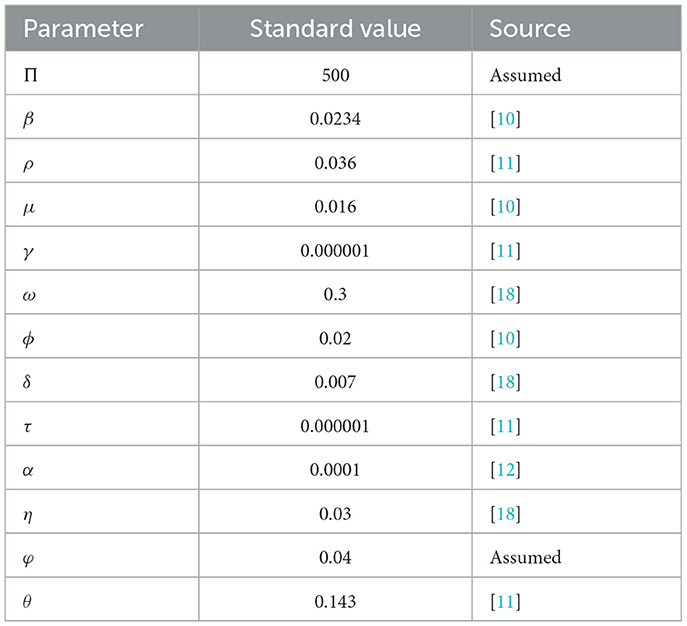
Table 3. Standard values for parameter of the system (1).

Therefore, we consider the following three strategies to determine the impact of each control on corruption reduction.

5.1 Strategy (i): strategy with only mass education (u₁) as prevention measure

Here, to optimize the objective function of the system (26), we used only mass education (u₁) on susceptible individuals while the control strategy (u₂) is not applied. As shown in Figure 2A, the number of exposed individuals decreases and then is constant over a fixed period of time. This indicates that the number of exposed population increases if there are no control strategies. Similarly, as shown in Figure 2B, we observe that the number of corrupt population decreases as the control strategy is used over a fixed period of time. In another way, the number of populations that participate in corruption activity increases if there are no control strategies. Therefore, we conclude that the mass education strategy plays an important role in the prevention of corruption activity.

Figure 2

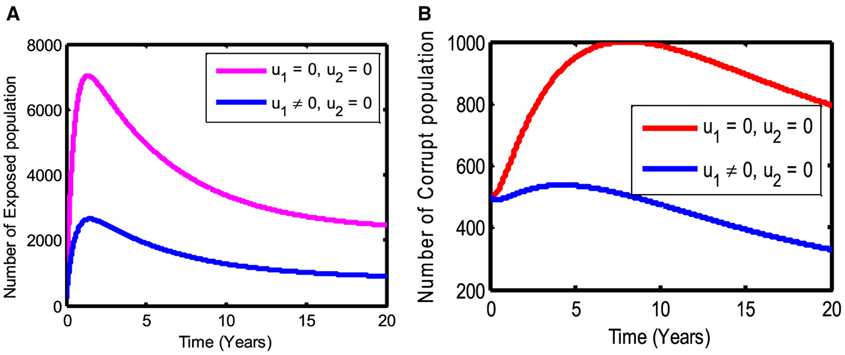
Figure 2. The effect of using only the mass education control strategy (u₁ ≠ 0).

5.2 Strategy (ii): strategy with only law enforcement (u₂) as reduction measure

Here, we use only the law enforcement (u₂) strategy on corrupted individuals in order to optimize the objective function of the system (26), while the control strategy (u₁) is equal to zero. We observe in Figure 3A that due to the law enforcement control strategy, the number of exposed individuals slowly decreased. However, as shown in Figure 3B, we observed that the number of corrupt population decreases significantly as the law enforcement control strategy is used. Therefore, we conclude that the law enforcement control strategy decreases both the number of exposed and corrupted populations. However, the number of corrupt populations spreads rapidly if the law enforcement control strategy is not applied.

Figure 3

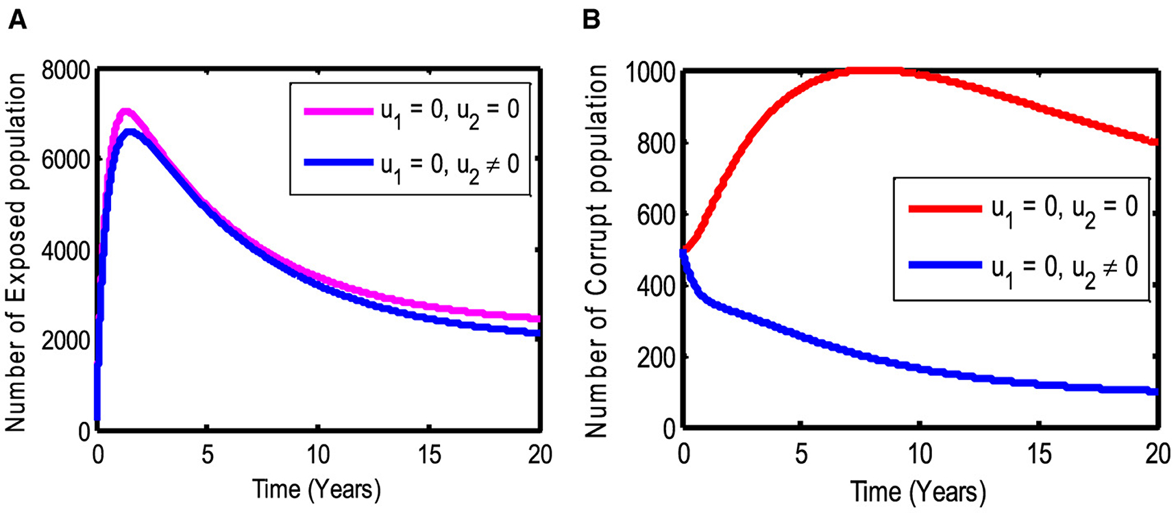
Figure 3. The effect of using only the law enforcement control strategy (u₂ ≠ 0).

5.3 Strategy (iii): Using both mass education (u₁) and law enforcement (u₂) control strategy

In this strategy, we use the combination of mass education (u₁) and law enforcement (u₂) control strategy on susceptible and corrupted individuals, respectively, that can optimize the objective function of the system of the study mentioned in the reference [26]. We observe in Figure 4A that the number of exposed individuals decreases significantly if we apply the control strategies, whereas if not, the number of exposed populations increases. Similarly, as shown in Figure 4B we show that the number of corrupted populations decreases significantly as control strategies are used, while the number of corrupted populations increases if there is no control strategy. Therefore, we conclude that applying both mass education and law enforcement strategies against corruption decreases both the number of exposed and corrupted populations in a given fixed period of time. This increases the number of jailed population, as shown in Figure 4C.

Figure 4

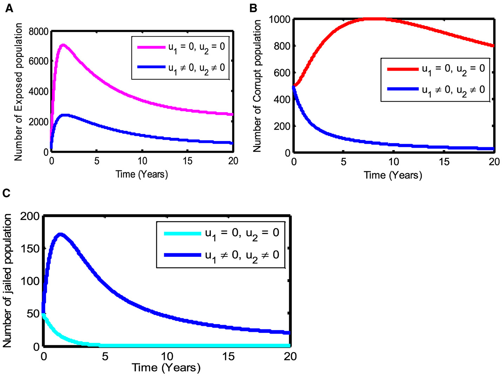
Figure 4. The effect of using both mass education (u₁ ≠ 0) and law enforcement (u₂ ≠ 0) strategies on the state variables.

6 Result, discussion, and conclusion

In this study, we develop a deterministic mathematical model for the transmission of corruption dynamics to study the effect of corruption in the population based on the corrupt status. To show that the formulated corruption model is mathematically and epidemiologically meaningful, we conducted a qualitative analysis of the model by showing that the solution of the model is positive and bounded. The basic reproduction number was calculated using the next-generation matrix method. The stability of the corruption-free and endemic equilibrium for the corruption dynamics model was analyzed in terms of the reproduction number. The analysis shows that for R₀ < 1, the corruption-free equilibrium point is asymptotically stable both locally and globally. It means that if the average number of new corrupted individuals generated by a single corrupted individual introduced into a susceptible population under any condition is less than one, the corruption will be minimized from the population. On the other hand, for whatever conditions if R₀ > 1, the corruption endemic equilibrium point is both locally and globally asymptotically stable. It means that corruption will increase in the population.

Furthermore, we extended the model to an optimal control strategy by incorporating two control variables, such as mass education and law enforcement. The necessary conditions for optimal controls such as existence and characterization were investigated with the help of Pontryagin's Maximum Principle. Finally, we have examined the numerical simulations of the optimal control model by considering individually and combining the control variables. Based on the results of the numerical analysis, we propose that using both mass education and law enforcement against corruption is the best strategy to minimize the number of exposed and corrupted populations. Therefore, anticorruption institutions and policymakers can use this finding as a good effort to reduce the corruption spread in the population. A significant and interesting aspect of the future study is to implement parameter estimation and cost-effectiveness analysis in the corruption dynamics model.

Data availability statement

The original contributions presented in the study are included in the article/supplementary material, further inquiries can be directed to the corresponding author.

Author contributions

TG: Formal analysis, Methodology, Software, Visualization, Writing – original draft, Writing – review & editing. AW: Conceptualization, Investigation, Methodology, Supervision, Validation, Visualization, Writing – review & editing. PK: Conceptualization, Data curation, Investigation, Methodology, Software, Supervision, Validation, Visualization, Writing – review & editing.

Funding

The author(s) declare that no financial support was received for the research, authorship, and/or publication of this article.

Acknowledgments

The authors sincerely acknowledge the Department of Mathematics, CNCS, Wollega University, and Samara University for their support during the study.

Conflict of interest

The authors declare that the research was conducted in the absence of any commercial or financial relationships that could be construed as a potential conflict of interest.

Publisher's note

All claims expressed in this article are solely those of the authors and do not necessarily represent those of their affiliated organizations, or those of the publisher, the editors and the reviewers. Any product that may be evaluated in this article, or claim that may be made by its manufacturer, is not guaranteed or endorsed by the publisher.

References

1. Grass D, Caulkins JP, Feichtinger G, Tragler G, Behrens DA. Optimal Control of Nonlinear Processes. Berlin, Heidelberg: Springer (2008).

Google Scholar

2. World Bank. Helping Countries Combat Corruption: The Role of the World Bank (1997).

Google Scholar

3. Cherrier B. Gunnar Myrdal and the scientific way to social democracy. Hist EconThought. (2009) 31:33–55. doi: 10.1017/S105383720909004X

Crossref Full Text | Google Scholar

4. Adela S, Bernard D, Grabova P. Corruption impact on economic growth: an empirical analysis. J Econ Dev Manag IT Finan Market. (2014) 6:57–77. Available online at: https://api.semanticscholar.org/CorpusID:156012079

Google Scholar

5. Saisana M, Saltelli A. Corruption Perceptions Index 2012 - Statistical Assessment. Luxembourg: Publications Office of the European Union (2012).

Google Scholar

6. Andvig JC. NUPI Working Paper Department of International Economics Crime, Poverty and Police Corruption in Non-Rich Countries (2008).

Google Scholar

7. Danford O, Kimathi M, Mirau S. Mathematical modelling and analysis of corruption dynamics with control measures in Tanzania. Math Informat. (2020) 19:57–79. doi: 10.22457/jmi.v19a07179

Crossref Full Text | Google Scholar

8. Eguda FY Oguntolu F, Ashezua T. Understanding the dynamics of corruption using mathematical modeling approach. Int J Innovat Sci Eng Technol. (2017) 4:190–7.

Google Scholar

9. Kebede G. Political corruption: political and economic state capture in Ethiopia. Eur Sci J. (2013) 9.

Google Scholar

10. Legesse L, Shiferaw F. Modelling corruption dynamics and its analysis. Ethiop J Sci Sustain Dev. (2018) 5:13–27. doi: 10.20372/ejssdastu:v5.i2.2018.34

Crossref Full Text | Google Scholar

11. Abdulrahman S. Stability analysis of the transmission dynamics and control of corruption. Pac J Sci Technol. (2014) 15:99–113.

Google Scholar

12. Nathan OM, Jackob KO. Stability analysis in a mathematical model of corruption in Kenya. Asian Res J Math. (2019) 15:1–15. doi: 10.9734/arjom/2019/v15i430164

Crossref Full Text | Google Scholar

13. Hattaf K. A new generalized definition of fractional derivative with non-singular kernel. Computation. (2002) 8:49. doi: 10.3390/computation8020049

Crossref Full Text | Google Scholar

14. Blanchaed P, Krueger A, Krueger T, Martin P. The epidemics of corruption. ArXiv. (2005).

Google Scholar

15. Brianzoni S, Coppier R, Michett R. Complex dynamics in a growth model with corruption in public procurement. Discrete Dyn Nat Soc. (2021) 2011:862396. doi: 10.1155/2011/862396

Crossref Full Text | Google Scholar

16. Athithan S, Ghosh M, Xue-Zhi L. Mathematical modeling and optimal control of corruption dynamics. Asian Eur J Math. (2018) 11:1850090. doi: 10.1142/S1793557118500900

Crossref Full Text | Google Scholar

17. Akanni JO, Akinpelu FO, Olaniyi S, Oladipo AT, Ogunsola AW. Modelling financial crime population dynamics: optimal control and cost-effectiveness analysis. Int J Dynam Control. (2020) 8:531–44. doi: 10.1007/s40435-019-00572-3

Crossref Full Text | Google Scholar

18. Akanni JO, Olaniyi S, Akinpelu FO. Global asymptotic dynamics of a nonlinear illicit drug use system. J Appl Math Comput. (2021) 66:39–60. doi: 10.1007/s12190-020-01423-7

Crossref Full Text | Google Scholar

19. Ibrahim OM, Okuonghae D, Ikhile MNO. A mathematical model of criminal gang rivalry: understanding the dynamics and implications. Results Control Optimiz. (2024) 14:100398. doi: 10.1016/j.rico.2024.100398

Crossref Full Text | Google Scholar

20. Hathroubi S. Epidemic Corruption: A Bio-economic Homology. Econstor (2013). Available online at: https://hdl.handle.net/10419/73558

Google Scholar

21. Alemneh HT. Mathematical modeling, analysis, and optimal control of corruption dynamics. Hind J Appl Math. (2020) 2002:5109841. doi: 10.1155/2020/5109841

Crossref Full Text | Google Scholar

22. Iheonu NO, Nwajeri UK, Omame A. A non-integer order model for Zika and Dengue co-dynamics with cross-enhancement. Healthc Anal. (2023) 4:100276. doi: 10.1016/j.health.2023.100276

Crossref Full Text | Google Scholar

23. Peter OJ, Panigoro HS, Abidemi A, Ojo MM, Oguntolu FA. Mathematical model of COVID-19 pandemic with double dose vaccination. Acta Biotheor. (2023) 71:9. doi: 10.1007/s10441-023-09460-y

PubMed Abstract | Crossref Full Text | Google Scholar

24. Gutema TW, Wedajo AG, Koya PR. Sensitivity and bifurcation analysis of corruption dynamics model with control measure. Int J Math Ind. doi: 10.1142/S2661335224500096

Crossref Full Text | Google Scholar

25. Dejene D, Worku T, Koya PR. Modeling the transmission and dynamics of COVID-19 using self-protection and isolation as control measures. Math Model Appl. (2020) 5:191–201. doi: 10.11648/j.mma.20200503.18

Crossref Full Text | Google Scholar

26. Van den Driessche P, Watmough J. Reproduction numbers and sub-threshold endemic equilibrium for compartmental models of disease transmission. Math Biosci. (2002) 180:29–48. doi: 10.1016/S0025-5564(02)00108-6

PubMed Abstract | Crossref Full Text | Google Scholar

27. Hailemichael DD, Geremew KE, Koya PR. Effect of vaccination and culling on the dynamics of rabies transmission from stray dogs to domestic dogs. Hind J Appl Math. (2022) 2022:2769494. doi: 10.1155/2022/2769494

Crossref Full Text | Google Scholar

28. Diekmann O, Heesterbeek JAP. Mathematical Epidemiology of Infectious Diseases: Model Building, Analysis and Integration. New York, NY: Wiley (2000).

Google Scholar

29. Osman M, Adu I, Isaac AK. Simple mathematical model for malaria transmission. J Adv Math Comp Sci. (2017) 25:1–24. doi: 10.9734/JAMCS/2017/37843

Crossref Full Text | Google Scholar

30. LaSalle JP. The Stability of Dynamical Systems. Philadelphia, PA: SIAM (1976).

Google Scholar

31. Gumel A. Introduction to dynamical system in mathematical epidemiology. In: Icmcsnuc Workshop, Abuja, Nigeria (2007).

Google Scholar

32. Goswami NK, Olaniyi S, Abimbade SF, Chuma FM. A mathematical model for investigating the effect of media awareness programs on the spread of COVID-19 with optimal control. Healthc Anal. (2024) 5:100300. doi: 10.1016/j.health.2024.100300

Crossref Full Text | Google Scholar

33. Olaniyi S, Kareem GG, Abimbade SF, Chuma FM, Sangoniyi SO. Mathematical modelling and analysis of autonomous HIV/AIDS dynamics with vertical transmission and nonlinear treatment. Iran J Sci. (2024) 48:181–92. doi: 10.1007/s40995-023-01565-w

Crossref Full Text | Google Scholar

34. Lenhart S, Workman JT. Optimal Control Applied to Biological Models, 1st Edn. Chapman and Hall/CRC (2007). p. 274

Google Scholar

35. Fleming WH, Rishel RW. Deterministic and Stochastic Optimal Control, Vol. 1. New York, NY: Springer Science & Business Media (2012).

Google Scholar

36. Wangari IM, Olaniyi S, Lebelo RS, Okosun KO. Transmission of COVID-19 in the presence of single-dose and double-dose vaccines with hesitancy: mathematical modeling and optimal control analysis. Front Appl Math Stat. (2023) 9:1292443. doi: 10.3389/fams.2023.1292443

Crossref Full Text | Google Scholar

37. Duressa Keno T, Mosisa Legesse F. Modelling and optimal control strategies of corruption dynamics. Appl Math Inform Sci. (2023) 17:67383. doi: 10.18576/amis/170416

Crossref Full Text | Google Scholar

38. Pontryagin LS, Boltyanskii VG, Gamkrelidze RV, Mischenko EF. The Mathematical Theory of Optimal Processes. New York, NY: Wiley Interscience (1962).

Google Scholar

39. Hailemichael DD, Edessa GK, Koya PR. Mathematical modeling of dog rabies transmission dynamics using optimal control analysis. Contemp Math. (2023) 4:296–319. doi: 10.21203/rs.3.rs-2682230/v1

Crossref Full Text | Google Scholar

40. Coddington EA, Levinson N. Theory of Ordinary Differential Equations. New York, NY: Tata McGraw-Hill Education (1955).

Google Scholar

41. Fantaye AK, Birhanu ZK. Mathematical model and analysis of corruption dynamics with optimal control. J Appl Math. (2022) 2022:8073877. doi: 10.1155/2022/8073877

Crossref Full Text | Google Scholar

42. Abidemi A, Olaniyi S, Adepoju OA. An explicit note on the existence theorem of optimal control problem. J Phys Conf Ser. (2022) 2199:012021. doi: 10.1088/1742-6596/2199/1/012021

Crossref Full Text | Google Scholar