Mathematical modeling and optimal control of multi-strain COVID-19 spread in discrete time

1 Introduction

Optimal Control Theory is a significant framework for optimizing dynamic systems. It was developed in the mid-twentieth century to find the best way to control systems over time while considering constraints and specific goals. Dynamic programming was introduced by Richard Bellman in the 1950's, and Lev Pontryagin developed the maximum principle in the 1960's, both of which were breakthroughs in the field. Since its inception, optimal control theory has become increasingly important in various fields, including engineering, epidemiology, and economics, owing to advancements in computing and mathematics. It is a crucial tool for decision making and improving system performance, making it essential for designing and optimizing dynamic processes.

In epidemiology, the optimal control theory is a valuable tool for enhancing control strategies against infectious diseases. Unlike conventional methods, which often rely on fixed interventions, optimal control theory adopts a dynamic approach that considers changing control measures over time. By considering factors such as transmission rates, intervention costs, and resource limits, optimal control models can identify strategies that maximize intervention impact while minimizing costs. This perspective provides a more comprehensive understanding of how epidemics work, which helps identify the best timing and intensity for interventions. Consequently, optimal control theory can lead to more adaptable, efficient, and personalized strategies that ultimately help manage and contain infectious diseases more effectively in populations. There have been several studies that utilized this method, such as Zakary et al. [1] who provided a comprehensive assessment of the impact of the Ebola virus and examined strategies for combating it using the optimal control approach. This approach also plays a role in transferring knowledge and raising awareness about serious diseases. Laarabi et al. [2] utilized a mathematical model of an SIR epidemic model with a saturated incidence rate and used optimal vaccination strategies to reduce the number of infected individuals and susceptible people while increasing the number of recovered individuals. Furthermore, many studies have focused on continuous modeling [3–7].

In this research, we employ discrete-time modeling, which is highly applicable in practical contexts. This is because numerous real systems naturally operate in discrete time, making discrete-time modeling a more precise representation. The accuracy of this method enhances the usefulness of the results in real-world situations, allowing for more effective decision-making in diverse circumstances. The data collected for this study were obtained at regular intervals, such as daily, weekly, monthly, or annual periods. Furthermore, providing treatment and medication for infected individuals and administering vaccinations for susceptible individuals were also conducted at specific times. Additionally, the use of discrete-time models streamlines the mathematical analysis by avoiding the intricate issues encountered in continuous-time modeling, such as the need to choose functional domains and ensure solution uniformity. Discrete-time models operate at precise intervals, such as days, weeks, months, or years. The discrete nature of these time intervals guarantees solution uniformity.

The appropriateness of numerical simulation methods for accurately simulating discrete-time optimal control systems and the computational efficiency of these methods for implementing discrete-time optimal control models are examined. Several studies have been conducted on the discrete-time modeling of dynamic systems. For instance, Kouidere et al. [8] proposed a discrete mathematical model that described the dynamics of a population of diabetics, emphasizing the impact of the living environment, such as unhealthy food and poor health habits, on diabetics without complications. El Bhih et al. [9] presented a study on optimal control strategies for a discrete model of the spread of Novel Coronavirus Disease, where the population is categorized into six compartments, representing different stages of infection, and an optimal strategy is proposed to combat the spread, utilizing controls such as media and education for sensitization and prevention, home quarantine for infected individuals, hospital quarantine for those with complications, and specialized hospital quarantine for individuals with multiple health conditions requiring breathing assistance. Balatif et al. [10] introduced a discrete mathematical model capturing citizens' dynamics and electoral behavior during awareness programs or election campaigns. The authors El Bhih et al. [11] proposed a mathematical model to analyze the spread of rumors in a social network. This model comprises four compartments, each representing a subpopulation's reaction to the rumor. They introduced control measures to curb the spread of the rumor. Toufga et al. [12] introduced a spatiotemporal discrete model for tuberculosis (TB), dividing individuals into susceptible, infected, exposed, and recovered categories. They proposed a control strategy that aims to reduce the number of infected and exposed individuals. Three controls were implemented: a public awareness campaign to educate the public about TB symptoms, signs, and treatments; chemoprophylaxis efforts for latently infected individuals; and treatment efforts for actively infected individuals. Several studies have focused on related topics [13–17].

The emergence and evolution of SARS-CoV-2 variants have posed significant challenges to global public health efforts combatting the COVID-19 pandemic. Notable variants include Alpha (B.1.1.7), first identified in the United Kingdom in September 2020 and designated as a variant of concern (VOC) in December 2020. Beta (B.1.351), which originated in South Africa in May 2020, was labeled as a VOC in December 2020. Gamma (P.1), which emerged in Brazil in November 2020, was designated as a VOC in January 2021. Delta (B.1.617.2), first detected in India in October 2020, was initially classified as a Variant of Interest (VOI) in April 2021 and later upgraded to a VOC in May 2021. Finally, the Omicron parent lineage (B.1.1.529), identified in multiple countries in November 2021, was initially classified as a variant under monitoring (VUM) in November 2021 and was later designated as a VOC in November 2021. These classifications and designations reflect the evolving understanding of SARS-CoV-2 variants and their potential impact on global public health, as documented by the World Health Organization. To access the WHO link and view the document on Historical working definitions and primary actions for SARS-CoV-2 variants [the World Health Organization].

Multiple studies have been conducted on the dynamics of population and transmission of different strains of COVID-19 with optimal control. Khajji et al. [18] proposed control strategies to reduce the number of infectious people and minimize the cost spent on vaccination and awareness programs. They divided the population into n+5 compartments: Susceptible, Exposed, Infected with i^th strain I_i, Hospitalized, Quarantined, and Recovered. The optimal control problem and related optimality conditions of the Pontryagin's maximum principle type were discussed to minimize the number of infected individuals. Gao et al. [19] developed a multi-strain model with infectious asymptomatic classes and applied it to COVID-19 dynamics in the US. They obtained the basic reproduction numbers for the two strains and interpreted their biological significance. Rigorous analyzes of the local and global stability of DFE were performed. Explicit formulas for two strain-dominant equilibria were also derived and analyzed for their local and global stability. Khajji et al. [14] formulated a multi-region discrete mathematical model that describes the dynamics of the transmission of COVID-19 between humans and animals in a region and between different regions. The strategies used in this study include awareness programs, health measures, and security campaigns. Efforts were made to encourage exposed and infected individuals to join quarantine centers. The last control is the disposal of infected animals to reduce the number of infected individuals and infected animals. Elqaddaoui et al. [20] developed a stochastic model that describes the propagation of COVID-19 variants, they assumed that the transmission rates of variants change over time due to the fluctuation of the weather and the temperature. Many studies have focused on this aspect [18, 19, 21–23].

1.1 Problem statement

Based on the advantages we previously mentioned of discrete-time mathematical modeling, as well as its compatibility with other mathematical theories, and its suitability for numerical simulation, in addition, noting the absence of the researches addressing this mathematical mechanism for monitoring the evolution and propagation of mutated strains of the COVID-19 virus. This study employed mathematical modeling in discrete time to track developments in the spread of COVID-19 variants. Due to the emergence of several COVID-19 variants that were mentioned previously, as mentioned on The World Health Organization website [24], in this study, the population is divided into n+2 compartments, S presents the susceptible, I_j presents the j^th strain, where j = 1, 2, 3, ..., n, and R represents the recovered people. In addition, we proposed two strategies: a vaccination strategy for the susceptible and a strategy of providing the appropriate treatment and medication for individuals infected with each strain separately to control and limit the spread of these strains at the minimum costs possible, deliberately avoiding the quarantine strategy because of its negative economic effects on individuals and different areas of economy, society, and life, and most studies used this strategy such that El Bhih et al. and Khajji et al. [9, 14, 18]. The goal was to evaluate the efficiency of the two strategies used to fight the spread of mutant strains by developing a discrete-time mathematical model that approximates a realistic picture of the spread of these strains by integrating the two aforementioned strategies into this model, which leads to an optimal control problem. In the followings sections, we used some mechanisms of optimal control theory, especially Pontryagin's maximum principle is used to obtain the desired results.

The remainder of this study is organized as follows. Section 2 introduces a discrete-time mathematical model, describes the model, and presents an optimal control problem. Section 3 describes the existence of optimal controls and characterizes them using Pontryagin's maximum principle in discrete time. Section 4 presents numerical simulations to further illustrate the model. Finally, Section 5 concludes the study.

2 A Mathematical model and description of the model

In this study, we assume that there are n mutant strains that are denoted by I₁, I₂, I₃, ..., I_n. Note that each strain I_i spreads at transmission rate β_i. The proportions P(i), S(i), I_j(i), (j = 1, 2, ..., n), and R(i) represent the number of the entire population, the number susceptible to infection, the number of people infected with strain I_j, and the number of people recovered respectively at time i. We consider the population denoted by $P(i)=S(i)+\sum _{j=1}^n{I}_j(i)+R(i)$. Figure 1 describes interactions between all compartments with their rates of this population.

Figure 1

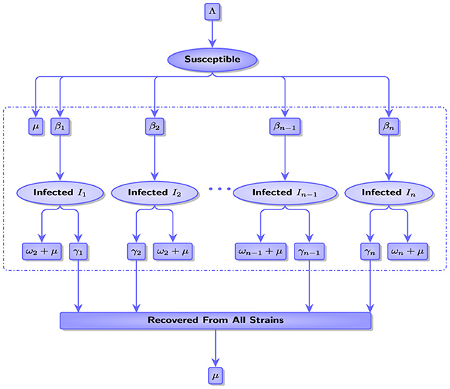
Figure 1. Description diagram of the multi-strains spread.

The following dynamic system represents the mathematical model that describes the spread of all mutant strains of this disease.

$\begin{array}{ll}\{\begin{array}{l}S(i+1)=\text{Λ}+\left(1-\mu \right)S(i)-{\displaystyle \sum _{j=1}^n{\beta }_j{I}_j(i)S(i).}\\ I_j(i+1)=\left(1-{\gamma }_j-{\omega }_j-\mu \right)I_j(i)+{\beta }_j{I}_j(i)S(i)j=1,\mathrm{2...},n.\\ R(i+1)={\displaystyle \sum _{j=1}^n{\gamma }_j{I}_j(i)+\left(1-\mu \right)R(i).}\end{array}& (1)\end{array}$

where μ is the natural death rate, Λ is the recruitment rate, β_j is the transmission rate of strain I_j, γ_j is the recovery rate from strain I_j, and ω_j is the death rate due to strain I_j. Figure 2 shows the spread of two strains in the natural state, that is, without any interventionist policy to limit the spread of these strains.

Figure 2

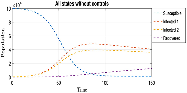
Figure 2. The states variables without controls.

2.1 The optimal control problem

This study aimed to evaluate the evolution of the spread of mutant strains using strategies that do not have negative effects on other areas to limit the excessive spread of these strains, such as the vaccination strategy and the strategy of providing appropriate treatment and medication while avoiding strategies that might have negative repercussions in other areas. In this study, we intentionally avoided the quarantine strategy due to its negative impacts on the economic sector for both individuals and society and the service sector and other areas. The important role of this study is to assess the efficiency of both strategies, vaccination u, and the provision of appropriate treatment and medication v_j for strain I_j in limiting the spread of mutant strains, without relying on quarantine strategy measures. We incorporate both strategies into this model (Equation 1). Then, we obtain the following:

$\begin{array}{ll}\{\begin{array}{l}S(i+1)=\Lambda +(1-\mu )S(i)-{\displaystyle \sum _{j=1}^n{\beta }_j}{I}_j(i)S(i)-u(i)S(i).\\ I_j(i+1)=(1-{\gamma }_j-{\omega }_j-\mu )I_j(i)+{\beta }_j{I}_j(i)S(i)-v(i{)}_j{I}_j(i)\\ j=1,\mathrm{2...},n.\\ R(i+1)={\displaystyle \sum _{j=1}^n{\gamma }_j}{I}_j(i)+(1-\mu )R(i)+{\displaystyle \sum _{j=1}^n{v}_j}(i)I_j(i).\end{array}& (2)\end{array}$

The quantities S(0) = S₀, I_j(0) = I_{j, 0}, (j = 1, 2....n), and R(0) = R₀ are the initial conditions.

The objective function is defined, and the purpose of the optimal control problem is to find the control inputs that minimize this objective function while satisfying System Dynamic Equation (2) and its initial conditions.

$\begin{array}{l}J(u,v_1,v_2\mathrm{...},v_n)\\ ={\displaystyle \sum _{i=1}^{T-1}\left({\displaystyle \sum _{j=1}^n{A}_j{I}_j(i)-BR(i)+\frac{1}{2}C{u}^2(i)+\frac{1}{2}}{\displaystyle \sum _{j=1}^n{D}_j{v}_j^2(i)}\right)}\\ +{\displaystyle \sum _{j=1}^n{A}_j}{I}_j(T)-BR(T)& (3)\end{array}$

where A_j > 0, B > 0, C > 0, and D_j > 0 for j ∈ {, 1, ...T} are cost coefficients. We chose these constants to weigh their relative importance of I₁(i), I₂(i), ..., I_n(i), R(i), u(i), v₁(i), v₂(i), ..., and v_n(i) at time i, and T is the final time. Our objective is to reduce the number of infected persons while also reducing systemic expenses by striving to maximize the number of people recovered from each I_j strain. In other words, we are looking for the optimal control $(u^{*},v_1^{*},v_2^{*}...,v_n^{*})$ such that:

$J(u^{*},v_1^{*},v_2^{*}...,v_n^{*})\le J(u,v_1,v_2...,v_n),\forall u\in U,\forall v_j\in V_j.$

where U and V_j, j = 1, 2..., n are admissible control sets defined as follows:

$U=\{u:u(i)\in [0,u_{max}],i\in [0,T-1]\}.$

$V_j=\{v_j:v_j(i)\in [0,v_j^{max}],i\in [0,T-1]\},j=1,2,\mathrm{.....}n.$

2.2 Existence of the optimal control

The sufficient condition for the existence of an optimal controls for problem (Equation 2) comes from the following theorem.

Theorem 2.1. There exist the optimal controls $(u^{*},v_1^{*},v_2^{*}...,v_n^{*})$ such that:

$J(u^{*},v_1^{*},v_2^{*}...,v_n^{*})\le J(u,v_1,v_2...,v_n),\forall u\in U,\forall v_j\in V_j.$

subject to the discrete-time control system (Equation 2) with initial conditions.

Proof: Because the number of time steps is finite and the coefficients of all the states of the equations are bounded, S = (S₀, S₁, ..., S_T), for j = 1, 2, ..., n, we have $I_j=(I_j^0,I_j^1,...,I_j^T)$ and R = (R₀, R₁, ..., R_T) are uniformly bounded for all u ∈ U and v_j ∈ V_j, j = 1, 2, ..., n. Thus, J(u, v₁, v₂..., v_n) is bounded for all u ∈ U and v_j ∈ V_j, j = 1, 2, ..., n. Because J(u, v₁, v₂..., v_n) is bounded,

$\underset{u\in U,(v_1,v_2,\mathrm{...},v_n)\in {\displaystyle \prod _{j=1}^n{V}_j}}{\inf }J(u,v_1,v_2\mathrm{...},v_n)\text{ is finite}.$

Moreover, there exists a sequence $(u^k,v_1^k,v_2^k...,v_n^k)$ with u ∈ U and v_j ∈ V_j, j = 1, 2, ..., n such that:

${\displaystyle \underset{k\to +\infty }{lim}}J(u^k,v_1^k,v_2^k...,v_n^k)={\displaystyle \underset{u\in U,(v_1,v_2,...,v_n)\in {\displaystyle \prod _{j=1}^n}{V}_j}{inf}}J(u,v_1,v_2...,v_n)$

and the corresponding sequences of the states $S^k,I_1^k,I_2^k,...,I_n^k$, and R^k. Because there are a finite number of uniformly bounded sequences, there exist $(u^{*},v_1^{*},v_2^{*}...,v_n^{*})$, u ∈ U, v_j ∈ V_j with j = 1, 2, ..., n and $S^{*},I_1^{*},I_2^{*},...,I_n^{*}$, and R^* ∈ ℝ^T+1 such that, on a subsequence, $(u^k,v_1^k,v_2^k...,v_n^k)\to (u^{*},v_1^{*},v_2^{*}...,v_n^{*})$ ,$S^k\to S^{*},I_1^k\to I_1^{*},I_2^k\to I_2^{*},...,I_n^k\to I_n^{*}$, and R^k→R^*. In the last, due to the finite dimensional structure of system (Equation 2) and the objective function, J(u, v₁, v₂..., v_n) and $(u^{*},v_1^{*},v_2^{*}...,v_n^{*})$ are optimal controls with corresponding states $S^{*},I_1^{*},I_2^{*},...,I_n^{*}$, and R^*. Therefore :

${\displaystyle \underset{u\in U,(v_1,v_2,...,v_n)\in {\displaystyle \prod _{j=1}^n}{V}_j}{inf}}J(u,v_1,v_2...,v_n)hasbeenachieved.$

We utilized the discrete form of Pontryagin's maximum principle, as detailed in references [25–28]. The main concept involves introducing a co-state function that links the set of difference equations representing the system to the objective function. This linkage results in the creation of the Hamiltonian function. Essentially, this principle transforms the task of determining the optimal control to enhance the objective function (Equation 3) by considering the state difference equation with an initial condition. The objective is to identify the control that optimizes the Hamiltonian at each point concerning the control, so the Hamiltonian H at time step k is defined as follows:

$\begin{array}{ll}{H}_k={\displaystyle \sum _{j=1}^n}{A}_j{I}_j(k)-BR(k)+\frac{1}{2}C{u}^2(k)+\frac{1}{2}{\displaystyle \sum _{j=1}^n}{D}_j{v}_j^2(k)+{\displaystyle \sum _{j=1}^{n+2}}{\lambda }_{j,k+1}{f}_{j,k+1}& (4)\end{array}$

where f_{j, k+1} represents the right side of the equation in a dynamic system (Equation 2) of the j^th state variable at time step k+1.

By replacing f_{j, k+1} with its expression found in system (Equation 2) in the Hamiltonian (Equation 4) we get:

$\begin{array}{l}{H}_k={\displaystyle \sum _{j=1}^n{A}_j{I}_j(k)-BR(k)+\frac{1}{2}C{u}^2(k)+\frac{1}{2}{\displaystyle \sum _{j=1}^n{D}_j{v}_j^2(k)+{\lambda }_{1,k+1}}}\\ \left(\Lambda +(1-\mu )S(k)-{\Sigma }_{j=1}^n{\beta }_j{I}_j(k)S(k)-u(k)S(k)\right)\\ +{\displaystyle \sum _{j=2}^{n+1}{\lambda }_{j,k+1}}\\ \left(\left(1-{\gamma }_{j-1}-{\omega }_{j-1}-\mu \right)I_{j-1}(k)+{\beta }_{j-1}{I}_{j-1}(k)S(k)-v{(k)}_{j-1}{I}_{j-1}(k)\right)\\ +{\lambda }_{n+2,k+1}\left({\displaystyle \sum _{j=1}^n{\gamma }_j{I}_j(k)+(1-\mu )R(k)+}{\displaystyle \sum _{j=1}^n{v}_j(k)I_j(k)}\right)\end{array}$

The states $S^{*},I_1^{*},I_2^{*},...,I_n^{*}$, and R^* describe the evolution of the system's state variables of (Equation 2) over time under the influence of the optimal controls $(u^{*},v_1^{*},v_2^{*}...,v_n^{*})$ . These state variables represent different compartments of a population.

Theorem 2.2. Given optimal controls $(u^{*},v_1^{*},v_2^{*}...,v_n^{*})$ and the associated solutions $S^{*},I_1^{*},I_2^{*},...,I_n^{*}$, and R^* of the corresponding states system (Equation 2),

there exists co-states λ_{1, k}, λ_{2, k}, ..., λ_{n+2, k} satisfying:

i) The co-state equations:

$\begin{array}{ll}\{\begin{array}{l}{\lambda }_{1,k}={\lambda }_{1,k+1}(1-\mu -{\displaystyle \sum _{j=1}^n{\beta }_j}{I}_j(k)-u(k))+{\displaystyle \sum _{j=2}^{n+1}{\lambda }_{j,k+1}}{\beta }_{j-1}{I}_{j-1}(k).\\ {\lambda }_{2,k}=A_1-{\lambda }_{1,k+1}{\beta }_{1}S(k)+{\lambda }_{2,k+1}({\beta }_{1}S(k)+1-{\gamma }_1-{\omega }_1-\mu -v_1(k))\\ +{\lambda }_{n+2,k+1}({\gamma }_1+v_1(k)).\\ {\lambda }_{3,k}=A_2-{\lambda }_{1,k+1}{\beta }_{2}S(k)+{\lambda }_{3,k+1}({\beta }_{2}S(k)+1-{\gamma }_2-{\omega }_2-\mu -v_2(k))\\ +{\lambda }_{n+2,k+1}({\gamma }_2+v_2(k)).\\ {\lambda }_{4,k}=A_3-{\lambda }_{1,k+1}{\beta }_{3}S(k)+{\lambda }_{4,k+1}({\beta }_{3}S(k)+1-{\gamma }_3-{\omega }_3-\mu -v_3(k))\\ +{\lambda }_{n+2,k+1}({\gamma }_3+v_3(k)).\\ .\\ .\\ .\\ {\lambda }_{n,k}=A_{n-1}-{\lambda }_{1,k+1}{\beta }_{n-1}S(k)+{\lambda }_{n,k+1}\\ ({\beta }_{n-1}S(k)+1-{\gamma }_{n-1}-{\omega }_{n-1}-\mu -v_{n-1}(k))\\ +{\lambda }_{n+2,k+1}({\gamma }_{n-1}+v_{n-1}(k))\\ {\lambda }_{n+1,k}=A_n-{\lambda }_{1,k+1}{\beta }_{n}S(k)+{\lambda }_{n+1,k+1}\\ ({\beta }_{n}S(k)+1-{\gamma }_n-{\omega }_n-\mu -v_n(k))+{\lambda }_{n+2,k+1}({\gamma }_n+v_n(k)).\\ {\lambda }_{n+2,k}=-B+{\lambda }_{n+2,k+1}(1-\mu )\end{array}& (5)\end{array}$

ii) The transversality conditions at time T:

$\begin{array}{l}{\lambda }_{1,T}=0\\ {\lambda }_{j,T}=A_{j-1},j=2,\mathrm{...},n+1\\ {\lambda }_{n+2,T}=-B\end{array}$

iii) The optimal controls:

For k = 0, 1, ..., T−1, the expressions of optimal controls $u^{*}(k),v_1^{*}(k),v_2^{*}(k),...,v_n^{*}(k)$ were obtained as follows:

$\begin{array}{l}{u}^{*}(k)=\min \left\{1,\max \left\{\frac{{\lambda }_{1,k+1}S(k)}{C},0\right\}\right\}\\ v_j^{*}(k)=\min \left\{1,\max \left\{\frac{{\lambda }_{n+2,k+1}{I}_j(k)-{\lambda }_{j+1,k+1}{I}_j(k)}{D_j},0\right\}\right\},\\ j=1,2,\mathrm{...},n.\end{array}$

Proof: i) For the co-state equations:

The Hamiltonian of the optimal control problem at time step k is given as follows:

$\begin{array}{l}{H}_k={\displaystyle \sum _{j=1}^n{A}_j{I}_j(k)-BR(k)+\frac{1}{2}C{u}^2(k)+\frac{1}{2}{\displaystyle \sum _{j=1}^n{D}_j{v}_j^2(k)+{\lambda }_{1,k+1}}}\\ \left(\Lambda +\left(1-\mu \right)S(k)-{\displaystyle \sum _{j=1}^n{\beta }_j{I}_j(k)S(k)-u(k)S(k)}\right)\\ +{\displaystyle \sum _{j=2}^{n+1}{\lambda }_{j,k+1}}\\ \left(\left(1-{\gamma }_{j-1}-{\omega }_{j-1}-\mu \right)I_{j-1}(k)+{\beta }_{j-1}{I}_{j-1}(k)S(k)-v{(k)}_{j-1}{I}_{j-1}(k)\right)\\ +{\lambda }_{n+2,k+1}\left({\displaystyle \sum _{j=1}^n{\gamma }_j{I}_j(k)+\left(1-\mu \right)R(k)}+{\displaystyle \sum _{j=1}^n{v}_j(k)I_j(k)}\right)\end{array}$

According to Pontryagin's maximum principle version in discrete time, given in Ding et al., Zhang and Shi, Guibout and Bloch, Hwang and Fan [25–28], by taking the derivatives of the Hamiltonian with respect to the state variables as follows:

$\begin{array}{l}{\lambda }_{1,k+1}=\frac{\partial H(k)}{\partial S(k)};{\lambda }_{j,k+1}=\frac{\partial H(k)}{\partial I_j(k)},j=1,2,\mathrm{...},n+1;\\ {\lambda }_{n+2,k+1}=\frac{\partial H(k)}{\partial D(k)}\end{array}$

With calculation, the co-state variables (Equation 5) will be obtained.

ii) For the transversality conditions:

Transversality conditions are necessary for ensuring that the terminal states of the system aligns with the objective of the optimization problem. We put $\text{Ψ}(T)={\displaystyle \sum _{j=1}^n{A}_j{I}_j(T)-BR(T)}$ by using also Pontryagin's maximum principle, in discrete time, such that:

$\begin{array}{l}{\lambda }_{1,T}=\frac{\partial \Psi (T)}{\partial S(T)}=0\\ {\lambda }_{j,T}=\frac{\partial \Psi (T)}{\partial I_j(T)}=A_{j,}j=2,3,\mathrm{...},n+1\\ {\lambda }_{n+2,T}=\frac{\partial \Psi (T)}{\partial R(T)}=-B\end{array}$

iii) For the optimal controls:

For k = 1, 2, ..., T−1, the optimal controls u(k), v_j(k), j = 1, 2, ..., n, can be solved from the following optimality condition:

$\frac{\partial H(k)}{\partial u(k)}=0$

With calculation we obtained

$u(k)=\frac{{\lambda }_{1,k+1}S(k)}{C}$

therefore

$\begin{array}{l}{u}^{*}(k)=\min \left\{1,\max \left\{\frac{{\lambda }_{1,k+1}S(k)}{C},0\right\}\right\}\hfill \end{array}$

And

$\frac{\partial H(k)}{\partial v_j(k)}=0,j=1,2,...,n$

With calculation, we obtained

$v_j(k)=\frac{{\lambda }_{n+2,k+1}{I}_j(k)-{\lambda }_{j+1,k+1}{I}_j(k)}{D_j},j=1,2,...,n.$

Therefore,

$\begin{array}{l}{v}_j^{*}(k)=\min \left\{1,\max \left\{\frac{{\lambda }_{n+2,k+1}{I}_j(k)-{\lambda }_{j+1,k+1}{I}_j(k)}{D_j},0\right\}\right\},\\ j=1,2,\mathrm{...},n.\end{array}$

3 Numerical simulation

This section explores the role of numerical simulations in analyzing the behavior and spread of two strains of an infectious disease. These simulations are crucial for enhancing our understanding of disease dynamics, assessing intervention strategies, and shaping effective public health policies, highlighting their critical importance in epidemiological research. In this section, we present a comprehensive analysis of the results obtained through numerical simulation of the optimality system in our control problem. Our methodology is characterized by defined initial conditions for the state variables and terminal conditions for the co-state variables, forming a two-point boundary value problem with specific boundary conditions at the start (time step i = 0) and end (time step i = T) of the process. To address this optimality, we used an iterative method. This begins with a forward simulation of the state system followed by a backward simulation of the co-state system. The procedure begins with a preliminary estimation of the control variables, which are then attractively refined based on their behavior in the simulation. This iterative process was maintained until a pattern of convergence in successive iterations was observed, signifying the achievement of an optimal solution. To facilitate and validate our findings, we developed and executed specialized MATLAB code tailored to the nuances of our control problem. The Table 1 presents the values of the parameters that were used in the numerical simulation.

Table 1

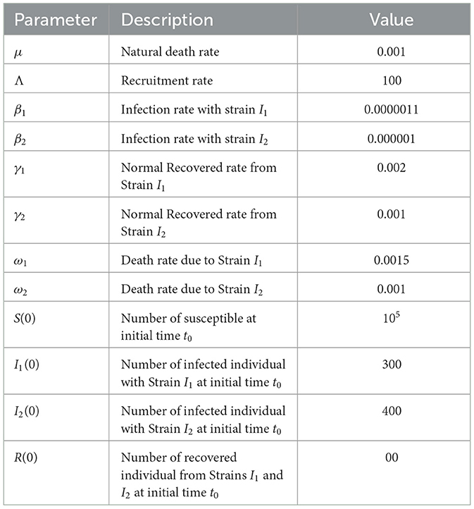
Table 1. Parameter values used in numerical simulation.

In this section, we employed three distinct control strategies, denoted as u(t), v₁(t), and v₂(t), with the primary objective of mitigating infections caused by both strains 1 and strain 2, while concurrently increasing the number of individuals who have recuperated. To identify the specific impact of each control strategy, we examine the following three scenarios:

• The first scenario applies only control u(t) and compares the results with those of the uncontrolled case.

• In the second scenario, we exclusively applied control u(t) with v₁(t) and v₂(t) separately, allowing for a comparative analysis with the uncontrolled case.

• The third scenario integrates all three control strategies u(t), v₁(t), and v₂(t), resulting in a comprehensive assessment of their combined impact.

3.1 Scenario 1: application the control u(t)

This scenario depends on the vaccination strategy u(t) for susceptible people, where u(t) represents the number of individuals vaccinated at moment t, and the following figures show the evolution of individuals in all compartments under the influence of this scenario.

Figure 3 shows two curves representing the progression of strain I₁. The blue curve illustrates the evolution of the strain in a scenario with no medical intervention, peaking at approximately 50,000 cases on day 85, followed by a gradual decline in infection rates. In contrast, the yellow curve shows the progression of the same strain under the vaccination strategy. This curve initially mirrors the trajectory of the blue curve for the first 40 days. Subsequently, a noticeable slowdown in the spread of the strain was observed, reflecting the protective impact of the vaccination. Approximately 70 days after the implementation of vaccination, the infection rate of the strain was halved compared with the non-vaccination scenario, indicating the efficacy of vaccination in mitigating the spread of this particular strain.

Figure 3

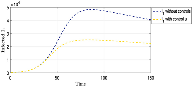
Figure 3. Strain I₁ without and with control u.

Figure 4 shows two curves representing the progression of the Strain I₂. The blue curve illustrates the evolution of the strain in the absence of any intervention to limit its spread, peaking at ~40,000 cases on day 90, followed by a gradual decline in infection rates. In contrast, the green curve depicts the progression of the same strain under vaccination strategy u. This curve initially mirrors the trajectory of the blue curve for the first 30 days. Subsequently, a noticeable slowdown in the spread of the strain is observed, reflecting the protective impact of vaccination. Approximately 70 days after the implementation of the vaccination strategy, the infection rate of the strain is halved compared with the non-vaccination scenario, indicating the efficacy of vaccination in mitigating the spread of this particular strain.

Figure 4

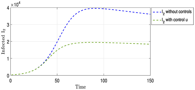
Figure 4. Strain I₂ without controls and with controls u.

Figure 5 contains two curves, where the Gold Curve shows the number of people who recovered from Strains I₁ and I₂ over time without using any treatment or infection control strategies. This curve indicates that the number of recoveries increased significantly over time; the explanation for this is that the lethality of these strains is not very dangerous. The brown curve represents the number of recoveries from these strains when a vaccination strategy is employed. This curve shows that the number of recoveries is significantly lower than that of the first curve. The explanation for this is that the vaccination strategy is effective and has prevented many people from contracting the disease, which might have been caused by the absence of vaccination and, after a number of them have recovered, would have been counted among the recoveries. Therefore, the number of recoveries was higher in the scenario without vaccination than in that with vaccination.

Figure 5

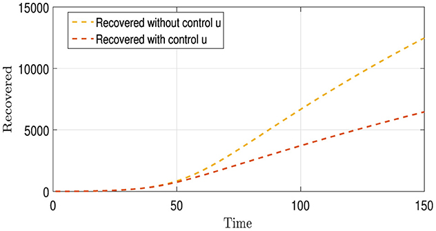
Figure 5. Recovered with and without control u.

3.2 Scenario 2: application the controls u(t) and v₁(t) for I₁ and v₂(t) for I₂

In addition to the vaccination strategy, this scenario depends on a strategy specific to the strain I₁ depends on providing the appropriate treatment and medications v₁(t) for individuals infected with strain I₁, and a strategy specific to the strain I₂ depends on providing the treatment and appropriate medications v₂(t) for individuals infected with strain I₂; the following figures show the evolution of number of infected people with each strain separately under the influence of scenario 2.

Figure 6 shows the two curves for Strain I1. The blue curve shows the natural development of Strain I1 in the absence of any intervention to limit its spread, as mentioned in the previous analysis. Conversely, the green curve displays the development of the strain under the influence of two strategies: vaccination and providing appropriate treatment and medication to those infected with this strain. From Figure 3, we observe that the period of overlap between the two curves becomes shorter than that in Figure 2. Additionally, there was a noticeable decrease in the number of infections, with a peak at ~16,000 cases on the 70th day, followed by a gradual decline. This pattern highlights the effectiveness of an integrated intervention strategy in reducing the spread of this strain.

Figure 6

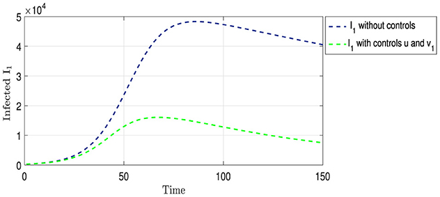
Figure 6. Strain I₁ without controls and with controls u, v₁.

Figure 7 shows two curves for Strain I₂. The curve colored in blue shows the natural development of this strain in the absence of any interventions to limit its spread, as mentioned in the previous analysis. In contrast, the olive curve displays the development of the strain under the influence of two strategies: vaccination u and appropriate treatment and medication v₂ for those infected with this strain. Figure 5 shows a shorter period of overlap between the two curves compared with Figure 4. The number of infections peaked at ~11,000 cases on the 60th day, followed by a significant reduction in the number of infected individuals, indicating the effectiveness of the integrated intervention strategy in reducing the spread of this strain.

Figure 7

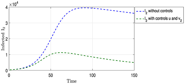
Figure 7. Strain I₂ without controls and with controls u, v₂.

3.3 Scenario 3: application the controls u(t), v₁(t) and v₂(t)

In this scenario, all strategies were simultaneously implemented. The following figures illustrate the evolution of the number of individuals in all compartments under this scenario.

Figure 8 contains two curves: The Gold Curve shows the number of people who have recovered from Strains I₁ and I₂ over time without using any treatment or infection control strategies, as previously mentioned above. The purple curve represents the number of recoveries from these two strains, involving both vaccination (u) and the provision of appropriate medication and treatment (v₁ and v₂ ) for each strain. From this figure, we observe that the purple curve is above the gold curve, in contrast to what we observed in Figure 5. This is due to the use of the controls v₁ and v₂, which increased the number of recoveries.

Figure 8

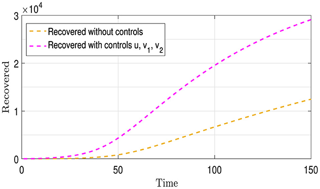
Figure 8. Recovered with and without control u, v₁, and v₂.

Figure 9 presents four distinct curves illustrating the progression of all population compartments, encompassing susceptible individuals (S), individuals infected with each strain (I₁ and I₂), and the recovered individuals (R). These trajectories are depicted under the influence of a comprehensive vaccination strategy (u) and the administration of appropriate medications (v₁ and v₂) tailored to each I₁ and I₂ category. In comparison to the baseline scenario depicted in Figures 1, 8 unveils a stark reduction in the number of infections for both strains, along with a notable and continuously increasing count of recovered individuals. This unequivocally underscores the efficacy of the implemented intervention strategies within this context.

Figure 9

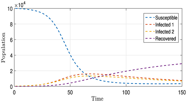
Figure 9. The states with controls u, v₁, and v₂.

4 Conclusion

In conclusion, this study introduced a mathematical model describing the dynamics of transmission for mutant strains of COVID-19 and proposed optimal strategies to combat their spread. Our strategies aim to minimize the number of infected individuals with each strain while maximizing the number of recovered individuals and minimizing associated costs. We incorporated two control strategies: a vaccination strategy for susceptible individuals and providing appropriate treatment and medication tailored to those infected with each strain separately. Through the application of Pontryagin's maximum principle in discrete time, we proved the existence of optimal controls and solved the optimality system using an iterative method. Furthermore, numerical simulations were conducted to evaluate the effectiveness of these strategies in managing the spread of mutant strains. Graphical representations were provided to illustrate the impact of control strategies on limiting the propagation of these strains. The simulations enabled us to compare different scenarios and observe the effectiveness of control strategies in a concrete manner. Despite the absence of the quarantine strategy, our findings indicate that these strategies effectively limit the spread of COVID-19 variants.

Data availability statement

The raw data supporting the conclusions of this article will be made available by the authors, without undue reservation.

Author contributions

AE: Writing - original draft, Writing - review & editing. AEB: Writing - original draft, Writing - review & editing. HL: Writing - original draft, Writing - review & editing. AA: Writing - original draft, Writing - review & editing. MR: Writing - original draft, Writing - review & editing.

Funding

The author(s) declare that no financial support was received for the research, authorship, and/or publication of this article.

Conflict of interest

The authors declare that the research was conducted in the absence of any commercial or financial relationships that could be construed as a potential conflict of interest.

Publisher's note

All claims expressed in this article are solely those of the authors and do not necessarily represent those of their affiliated organizations, or those of the publisher, the editors and the reviewers. Any product that may be evaluated in this article, or claim that may be made by its manufacturer, is not guaranteed or endorsed by the publisher.

References

1. Zakary O, Rachik M, Elmouki I. A multi-regional epidemic model for controlling the spread of Ebola: awareness, treatment, and travel-blocking optimal control approaches. Math Methods Appl Sci. (2017) 40:1265–79. doi: 10.1002/mma.4048

Crossref Full Text | Google Scholar

2. Laarabi H, Rachik M, Kaddar A. Optimal control of an epidemic model with a saturated incidence rate. Nonlin Anal. (2012) 17:448–59. doi: 10.15388/NA.17.4.14050

Crossref Full Text | Google Scholar

3. El Bhih A, Yaagoub Z, Rachik M, Allali K, Abdeljawad T. Controlling the dissemination of rumors and antirumors in social networks: a mathematical modeling and analysis approach. Eur Phys J Plus. (2024) 139:1–23. doi: 10.1140/epjp/s13360-023-04844-y

Crossref Full Text | Google Scholar

4. Goswami NK, Olaniyi S, Abimbade SF, Chuma FM. A mathematical model for investigating the effect of media awareness programs on the spread of COVID-19 with optimal control. Healthc Analyt. (2024) 2024:100300. doi: 10.1016/j.health.2024.100300

Crossref Full Text | Google Scholar

5. Castiglione F, Piccoli B. Cancer immunotherapy, mathematical modeling and optimal control. J Theoret Biol. (2007) 247:723–32. doi: 10.1016/j.jtbi.2007.04.003

PubMed Abstract | Crossref Full Text | Google Scholar

6. Danane J, Meskaf A, Allali K. Optimal control of a delayed hepatitis B viral infection model with HBV DNA–containing capsids and CTL immune response. Opt Contr Appl Methods. (2018) 39:1262–72. doi: 10.1002/oca.2407

Crossref Full Text | Google Scholar

7. Fantaye AK, Birhanu ZK. Mathematical model and analysis of corruption dynamics with optimal control. J Appl Math. (2022) 2022:1–16. doi: 10.1155/2022/3844885

Crossref Full Text | Google Scholar

8. Kouidere A, Balatif O, Ferjouchia H, Boutayeb A, Rachik M. Optimal control strategy for a discrete time to the dynamics of a population of diabetics with highlighting the impact of living environment. Discr Dyn Nat Soc. (2019) 2019:1–8. doi: 10.1155/2019/6342169

Crossref Full Text | Google Scholar

9. El Bhih A, Benfatah Y, Kouidere A, Rachik M. A discrete mathematical modeling of transmission of COVID-19 pandemic using optimal control. Commun Math Biol Neurosci. (2020). doi: 10.28919/cmbn/4780

Crossref Full Text | Google Scholar

10. Balatif O, Khajji B, Rachik M. Mathematical modeling, analysis, and optimal control of abstinence behavior of registration on the electoral lists. Discr Dyn Nat Soc. (2020) 2020:9738934. doi: 10.1155/2020/9738934

Crossref Full Text | Google Scholar

11. El Bhih A, Ghazzali R, Ben Rhila S, Rachik M, El Alami Laarroussi A. A discrete mathematical modeling and optimal control of the rumor propagation in online social network. Discr Dyn Nat Soc. (2020) 2020:1–12. doi: 10.1155/2020/4386476

Crossref Full Text | Google Scholar

12. Toufga H, Benahmadi L, Sakkoum A, Lhous M. Optimal control of a spatiotemporal discrete tuberculosis model. Int J Biomath. (2024) 2024:2350110. doi: 10.1142/S1793524523501103

Crossref Full Text | Google Scholar

13. Labzai A, Kouidere A, Khajji B, Balatif O, Rachik M. Mathematical modeling and optimal control strategy for a discrete time drug consumption model. Discr Dyn Nat Soc. (2020) 2020:1–10. doi: 10.1155/2020/5671493

Crossref Full Text | Google Scholar

14. Khajji B, Kada D, Balatif O, Rachik M. A multi-region discrete time mathematical modeling of the dynamics of COVID-19 virus propagation using optimal control. J Appl Math Comput. (2020) 64:255–81. doi: 10.1007/s12190-020-01354-3

PubMed Abstract | Crossref Full Text | Google Scholar

15. Gao Z. On discrete time optimal control: a closed-form solution. In: Proceedings of the 2004 American Control Conference, Vol. 1. IEEE (2004). p. 52–8. doi: 10.23919/acc.2004.1383578

Crossref Full Text | Google Scholar

16. Yakowitz S, Rutherford B. Computational aspects of discrete-time optimal control. Appl Math Comput. (1984) 15:29–45.

Google Scholar

17. Lhous M, Rachik M, Laarabi H, Abdelhak A. Discrete mathematical modeling and optimal control of the marital status: the monogamous marriage case. Adv Diff Eq. (2017) 2017:1–16. doi: 10.1186/s13662-017-1390-0

Crossref Full Text | Google Scholar

18. Khajji B, Boujallal L, Balatif O, Rachik M. Mathematical modelling and optimal control strategies of a multistrain COVID-19 spread. J Appl Math. (2022) 2022:9071890. doi: 10.1155/2022/9071890

Crossref Full Text | Google Scholar

19. Gao S, Shen M, Wang X, Wang J, Martcheva M, Rong L. A multi-strain model with asymptomatic transmission: application to COVID-19 in the US. J Theoret Biol. (2023) 565:111468. doi: 10.1016/j.jtbi.2023.111468

PubMed Abstract | Crossref Full Text | Google Scholar

20. Elqaddaoui A, El Bhih A, Laarabi H, Rachik M, Abta, A. A stochastic optimal control strategy for multi-strain COVID-19 spread. Commun Math Biol Neurosci. (2023) 2023:2052–541. doi: 10.28919/cmbn/8223

Crossref Full Text | Google Scholar

21. Otunuga OM. Analysis of multi-strain infection of vaccinated and recovered population through epidemic model: application to COVID-19. PLoS ONE. (2022) 17:e0271446. doi: 10.1371/journal.pone.0271446

PubMed Abstract | Crossref Full Text | Google Scholar

22. Arruda EF, Das SS, Dias CM, Pastore DH. Modelling and optimal control of multi strain epidemics, with application to COVID-19. PLoS ONE. (2021) 16:e0257512. doi: 10.1371/journal.pone.0257512

PubMed Abstract | Crossref Full Text | Google Scholar

23. Khyar O, Allali K. Global dynamics of a multi-strain SEIR epidemic model with general incidence rates: application to COVID-19 pandemic. Nonlin Dyn. (2020) 102:489–509. doi: 10.1007/s11071-020-05929-4

PubMed Abstract | Crossref Full Text | Google Scholar

24. The World Health Organization. Definitions (2019). Available online at: https://www.who.int/publications/m/item/historical-working-definitions-and-primary-actions-for-SARS-CoV-2-variants (accessed June 16, 2024).

Google Scholar

25. Ding W, Hendon R, Cathey B, Lancaster E, Germick R. Discrete time optimal control applied to pest control problems. Involve J Math. (2014) 7:479–89. doi: 10.2140/involve.2014.7.479

Crossref Full Text | Google Scholar

26. Zhang DC, Shi B. Oscillation and global asymptotic stability in a discrete epidemic model. J Math Anal Appl. (2003) 278:194–202. doi: 10.1016/S0022-247X(02)00717-5

Crossref Full Text | Google Scholar

27. Guibout V, Bloch A. A discrete maximum principle for solving optimal control problems. In: 2004 43rd IEEE Conference on Decision and Control (CDC)(IEEE Cat. No. 04CH37601), Vol. 2. IEEE (2004). p. 1806–11. doi: 10.1109/cdc.2004.1430309

Crossref Full Text | Google Scholar

28. Hwang CL, Fan LT. A discrete version of Pontryagin's maximum principle. Operat Res. (1967) 15:139–46. doi: 10.1287/opre.15.1.139

Crossref Full Text | Google Scholar