Application of story-wise shear building identification method to actual ambient vibration

Introduction

Much research interest has been directed recently to system identification (SI) of civil, mechanical, and aerospace structures in response to the increasing need of enhancement of safety and upgrade of ability of damage detection (or damage diagnosis) of various kinds of structures (Hart and Yao, 1977; Beck and Jennings, 1980; Hoshiya and Saito, 1984; Kozin and Natke, 1986; Agbabian et al., 1991; Koh et al., 1991; Ghanem and Shinozuka, 1995; Hjelmstad et al., 1995; Shinozuka and Ghanem, 1995; Doebling et al., 1996; Hjelmstad, 1996; Masri et al., 1996; Housner et al., 1997; Kobori et al., 1998; Johnson and Smyth, 2006; Nagarajaiah and Basu, 2009; Fujino et al., 2010; Ji et al., 2011). Such need results from the accelerated demand of rapid assessment on material aging issues and of continuing use of buildings after earthquakes. The Building Continuity Plan (BCP) and resilience-oriented design framework also supports the increasing need of advancement of structural health monitoring technologies. It is also well-recognized that SI plays an important and principal role in reducing gaps between the constructed structural systems and their structural design models (model refinement).

Basically, two kinds of branches of the SI technique are known. One is called the modal parameter SI, which is well-established, and another is called the physical parameter SI. The modal parameter SI is well-established and various types of research have been conducted and accumulated so far [for example, see Hart and Yao (1977) and Beck and Jennings (1980)]. Since the modal parameters are global parameters and stable in principle, many useful techniques have been proposed. In the modal parameter SI, for evaluating the natural frequency and damping ratio, the observations at two places at least (usually the base and the top) are necessary. Furthermore, for evaluating modal shape identification, the simultaneous observations (or interpolation from fewer observations) at many places are usually required that is often a cumbersome task in the modal parameter SI method. When the observations at all the floors of a building are possible, all story stiffnesses of the shear building model with known floor masses may be identified within an acceptable accuracy (Hjelmstad et al., 1995).

In contrast to such modal parameter SI, the physical parameter SI has been developed for direct identification of physical parameters (stiffness and damping coefficients). For example, Takewaki and Nakamura (2000; 2005) introduced a method based on the work by Udwadia et al. (1978). In that method, a shear building model is used and stiffness and damping coefficients of a specific story are identified directly from the floor accelerations just above and below the specific story. However, the method by Takewaki and Nakamura (2000; 2005) has a difficulty resulting from the small signal/noise (SN) ratio in the low frequency range and cannot be applied to ambient vibration data, e.g., micro-tremors, and to high-rise buildings with large height-to-width aspect ratios. The former problem has been a major and most difficult problem in the field of SI and the latter problem has been tackled by Minami et al. (2013) and Fujita et al. (2013) by using a shear-bending model.

Hernandez-Garcia et al. (2010a;b) have developed an interesting method of damage detection using a floor-by-floor approach to enhance the efficiency and accuracy of the identification results. Xing and Mita (2012) have devised a time-domain substructure damage identification method for shear buildings by focusing on a substructure consisting of one story. Zhang and Johnson (2013) have developed another substructure identification method for shear buildings, which considers the noise effect of recorded data on identification accuracy and utilizes an iterative inductive procedure from the top story. Furthermore, a combined method of the modal parameter SI and the physical parameter SI is also well used (for example, Shinozuka and Ghanem, 1995; Barroso and Rodriguez, 2004). After modal parameters are identified, physical parameters are determined by solving inverse problems in which the existence and uniqueness of solutions are principal problems. Takewaki and Nakamura (2009) have developed a method for identifying the temporal variation of modal properties of a base-isolated building during an earthquake by using the relation between auto-regressive eXogenous (ARX) model parameters and modal parameters.

The difficulty arising in the limit manipulation in the method by Takewaki and Nakamura (2000; 2005) has been overcome by introducing an ARX model in the previous paper (Maeda et al., 2011). The weakness of a small signal-to-noise (SN) ratio in the low frequency range in the method (Takewaki and Nakamura, 2000; 2005) has been avoided by using the ARX model and introducing new constraints on the ARX parameters. Another difficulty due to small vibration levels of micro-tremor has been tackled by introducing a combination of the ARX model, filtering in the frequency domain (low and high-cut filter), and averaging in the time domain (sequential time-window shift for Fourier transformation and averaging). In this paper, for obtaining reliable and stable identification of story stiffnesses, a practical procedure to decide the combination of the degree of ARX models and cut-off frequencies of filtering is investigated by applying a multi-objective optimization algorithm. It is shown that the previously proposed story-wise stiffness identification method is applicable in the new approaches to actual recorded data of an ambient vibration level with the help of this sophisticated combination.

System Identification Method for Physical Parameters of Shear Building Model

Governing Equations of Shear Building Model

Consider an N-story shear building model with viscous damping as shown in Figure 1. Let m_j and k_j denote the mass of the j-th floor and the story stiffness of the j-th story and let c_j be the viscous damping coefficient of the j-th story. Since the formulation in the frequency domain is appropriate in the present formulation, all the governing equations are expressed in the frequency domain. Let “i” denote the imaginary unit.

FIGURE 1

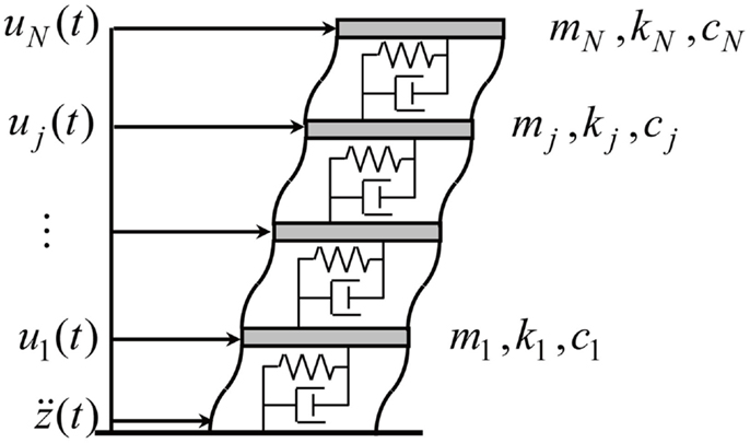
Figure 1. N-story shear building model with viscous damping.

Keeping the relations $\dot{U}\left(\omega \right)=\mathrm{i}\mathrm{\omega U}\left(\omega \right),$ Ü(ω) = −ω²U(ω) in mind, the equations of motion in the frequency domain for this shear building model subjected to the horizontal ground acceleration ü_g is expressed as:

$\left(-{\mathrm{\omega }}^{2}M+\mathrm{i}\mathrm{\omega }C+K\right)U\left(\mathrm{\omega }\right)=-\mathbf{\text{M1}}{\mathit{Ü}}_g\left(\mathrm{\omega }\right)$ (1)

where U(ω) and Ü_g(ω) are the Fourier transforms of the horizontal displacements u(t) = {u_j(t)} of floors relative to ground and the ground base acceleration ü_g, respectively. The vector 1 in the right-hand side of Eq. (1) denotes 1 = {1, 1, …, 1}^T. The mass, stiffness, and damping matrices of shear building model are defined by:

$\begin{array}{ll}\hfill & M=\mathrm{diag}\left(m_1,m_2,\cdots ,m_N\right),\end{array}$ (2a)

$\begin{array}{ll}\hfill & K=\left[\begin{array}{cccc}{k}_1+k_2& -k_2& & \\ -k_2& k_2+k_3& -k_3& \\ & & \ddots & \\ & & -k_N& k_N\\ \end{array}\right],\end{array}$ (2b)

$\begin{array}{ll}\hfill & \hfill & C=\left[\begin{array}{cccc}{\mathit{c}}_1+{\mathit{c}}_2& -{\mathit{c}}_2& & \\ -{\mathit{c}}_2& {\mathit{c}}_2+{\mathit{c}}_3& -{\mathit{c}}_3& \\ & & \ddots & \\ & & -{\mathit{c}}_{\mathit{N}}& {\mathit{c}}_{\mathit{N}}\\ \end{array}\right]\end{array}$ (2C)

The transfer function T(ω) can be defined from Eq. (1) as the ratio of the horizontal displacement to the ground acceleration.

$T\left(\mathrm{\omega }\right)\equiv U\left(\mathrm{\omega }\right)∕{\mathit{Ü}}_g\left(\mathrm{\omega }\right)=-A{\left(\mathrm{\omega }\right)}^{-1}\mathbf{\text{M1}}$ (3)

where A(ω) = −ω²M + i ωC + K.

Sub-System Identification Based on Identification Function

Based on the mathematical formulation for the SI of the physical parameters (Takewaki and Nakamura, 2000), the story stiffness and damping coefficient can be expressed by using the limit manipulation of the identification function f_j(ω) for ω → 0. The story stiffness and damping coefficient are derived as:

$k_j=\underset{\mathrm{\omega }\to 0}{lim}\left(M_j\times \mathrm{Re}\left[-{\mathrm{\omega }}^2\frac{\left({\mathit{Ü}}_g+{\mathit{Ü}}_j\right)}{\left({\mathit{Ü}}_g+{\mathit{Ü}}_{j-1}\right)-\left({\mathit{Ü}}_g+{\mathit{Ü}}_j\right)}\right]\right)$ (4)

$c_j=\underset{\mathrm{\omega }\to 0}{lim}\left(M_j\times \frac{d}{d\mathrm{\omega }}\left\{\mathrm{Im}\left[-{\mathrm{\omega }}^2\frac{\left({\mathit{Ü}}_g+{\mathit{Ü}}_j\right)}{\left({\mathit{Ü}}_g+{\mathit{Ü}}_{j-1}\right)-\left({\mathit{Ü}}_g+{\mathit{Ü}}_j\right)}\right]\right\}\right)$ (5)

where $M_j={\sum }_{i=j}^N{m}_i$. Referring Takewaki and Nakamura (2000), the identification function can be defined by:

$f_j\left(\mathrm{\omega }\right)\equiv -{\mathrm{\omega }}^2{M}_j\frac{{\mathit{Ü}}_g+{\mathit{Ü}}_j}{{\mathit{Ü}}_{j-1}-{\mathit{Ü}}_j}$ (6)

In Eqs (4–6), Ü₀ = 0. From Eqs (4) and (5), it is concluded that the story stiffness and damping coefficient can be derived only from the accelerations just above and below floors of the object story in the previously proposed identification method (Takewaki and Nakamura, 2000).

Identification of Stiffness and Damping Coefficient using ARX Model

Taylor Series Expansion of Transfer Function Using ARX Parameters

In the previous SI method (Takewaki and Nakamura, 2000; 2005) for shear building models as formulated in Eqs (4) and (5), the limit manipulation of the identification function f_j(ω) for ω → 0 was needed. However, when the identification functions are evaluated from the raw data such as actual vibration testing data, it is often the case that the identification functions become unstable and exhibits a large variability in the low frequency range. To overcome this difficulty, an ARX model is introduced, which is a time-domain model. The reliability of the ARX model in this direction has been confirmed and the applicability of the ARX model to shear building models and shear-bending models has been demonstrated in Maeda et al. (2011) and Minami et al. (2013).

The identification function f_j(ω) defined by Eq. (6) can be rewritten by introducing the transfer function G_{j, j−1}(ω) between j-th and (j − 1)-th floors as

$f_j\left(\mathrm{\omega }\right)=-\frac{{\mathrm{\omega }}^2{M}_j}{\frac{1}{G_{j,j-1}\left(\mathrm{\omega }\right)}-1}$ (7)

where G_{j, j−1}(ω) ≡ (Ü_g + Ü_j)/(Ü_g + Ü_j−1). The reason of the unstable phenomenon of the identification function in the low frequency range can be understood from Eq. (7). From the theoretical investigation, the limit value of the transfer function G_{j, j−1}(ω) at ω = 0 should be G_{j, j−1}(0) = 1, because the j-th floor and (j − 1)-th floor move identically at ω → 0. Therefore, the limit value of the denominator of the identification function 1/G_{j, j − 1}(ω) − 1 for ω → 0 is zero. Furthermore, the limit value of the numerator of the identification function ω²M_j for ω → 0 is also zero. For these reasons, the limit value of the identification function f_j(ω) for ω → 0 is theoretically indefinite.

By using ARX parameters, the transfer function can also be expressed as (see Appendix)

$G_{j,j-1}\left(\mathrm{\omega }\right)=\frac{b_1{e}^{-\mathrm{i}\mathrm{\omega }{T}_0}+\cdots +b_n{e}^{-\mathrm{i}n\mathrm{\omega }{T}_0}}{1+a_1{e}^{-\mathrm{i}\mathrm{\omega }{T}_0}+\cdots +a_n{e}^{-\mathrm{i}n\mathrm{\omega }{T}_0}}$ (8)

For evaluation of the limit value of the transfer function G_{j, j − 1}(ω) for ω → 0, the formulation of the Taylor series expansion of the transfer function G_{j, j−1}(ω) is meaningful. The Taylor series expansion of the transfer function G_{j, j − 1}(ω) in terms of ARX parameters can be defined as

$G_{j,j-1}\left(\mathrm{\omega }\right)\simeq A_0+A_1\mathrm{\omega }+A_2{\mathrm{\omega }}^2+\cdots$ (9)

Considering the relationship of ARX parameters in Eq. (8) and the coefficients of the Taylor series expansion in Eq. (9), the coefficients A₀, A₁, A₂ of the Taylor series expansion can be formulated in terms of the ARX parameters {a_k}, {b_k} as follows.

$A_0=b_{\mathrm{sum}}∕\left(1+a_{\mathrm{sum}}\right)$ (10)

$A_1=\mathrm{i}{T}_0\frac{\begin{array}{c}\left(1+a_{\mathrm{sum}}\right){\sum }_{k=1}^{n-1}\left(n-k\right)b_k-b_{\mathrm{sum}}\left\{n+{\sum }_{k=1}^{n-1}\left(n-k\right)a_k\right\}\hfill \end{array}}{{\left(1+a_{\mathrm{sum}}\right)}^2}$ (11)

$\begin{array}{llll}\hfill A_2& =-\frac{{T_0}^2}{2}\left[\frac{{\sum }_{k=1}^{n-1}{\left(n-k\right)}^2{b}_k}{1+a_{\mathrm{sum}}}\right.-\frac{b_{\mathrm{sum}}\left\{n^2+{\sum }_{k=1}^{n-1}{\left(n-k\right)}^2{a}_k\right\}}{{\left(1+a_{\mathrm{sum}}\right)}^2}& \hfill & \\ \hfill & -\frac{2{\sum }_{k=1}^{n-1}\left(n-k\right)b_k\left\{n+{\sum }_{k=1}^{n-1}\left(n-k\right)a_k\right\}}{{\left(1+a_{\mathrm{sum}}\right)}^2}\left.+\frac{2b_{\mathrm{sum}}{\left\{n+{\sum }_{k=1}^{n-1}\left(n-k\right)a_k\right\}}^2}{{\left(1+a_{\mathrm{sum}}\right)}^3}\right]\end{array}$ (12)

where $a_{\mathrm{sum}}\equiv {\sum }_{k=1}^n{a}_k,b_{\mathrm{sum}}\equiv {\sum }_{k=1}^n{b}_k.$

By introducing the real and imaginary parts of A_j as $A_j=A_j^R+\mathrm{i}{A}_j^I$ and substituting the properties of the real and imaginary parts of A_j into Eqs (10–12), the transfer function can be reduced to:

$G_{j,j-1}\left(\mathrm{\omega }\right)\simeq \left(A_0^R+A_2^R{\mathrm{\omega }}^2+\cdots \right)+\mathrm{i}\left(A_1^I\mathrm{\omega }+A_3^I{\mathrm{\omega }}^3+\cdots \right)$ (13)

Constraints on ARX Parameters Derived from the Limit Value of Taylor Series Expansion of Transfer Function

As mentioned in the previous section, it is meaningful to note that Eqs (14a,b) can be derived from the mechanical interpretation, i.e., the j-th floor and ( j − 1)-th floor move identically at ω → 0 and G_{j, j − 1}(ω) should not include linear terms of ω judging from Eqs (4–6).

$\begin{array}{ll}\hfill & \underset{\mathrm{\omega }\to 0}{lim}\mathrm{Re}\left\{G_{j,j-1}\left(\mathrm{\omega }\right)\right\}=1,\end{array}$ (14a)

$\begin{array}{ll}\hfill & \underset{\mathrm{\omega }\to 0}{lim}\frac{d}{d\mathrm{\omega }}\mathrm{Im}\left\{G_{j,j-1}\left(\mathrm{\omega }\right)\right\}=0\end{array}$ (14b)

From Eqs (13) and (14a, b), $A_0^R=1,A_1^I=0$. Furthermore, by substituting these equations into Eqs (10) and (11), the following equations can be derived.

${\sum }_{k=1}^n{a}_k+1={\sum }_{k=1}^n{b}_k$ (15)

${\sum }_{k=1}^{n-1}\left(n-k\right)b_k=n+{\sum }_{k=1}^{n-1}\left(n-k\right)a_k$ (16)

For enhancing the reliability of the proposed SI method, these relations will be used as the constraints in the estimation of the ARX parameters. It is found that Eq. (15) is a linear equation for the ARX parameters. A batch processing least-squares estimation method (see Appendix) (Adachi, 2009) provides:

$\mathbf{\text{R}}\mathrm{\theta }=\mathbf{\text{f}}$ (17)

R, θ, and f are defined in Appendix.

By applying the Lagrange multiplier method, the linear constraint can be incorporated into the batch processing least-squares estimation method as p^Tθ = −1 where p = {1, …, 1, −1, …, −1}^T. Therefore, the present method is reduced to the problem for solving the following equations.

$\left[\begin{array}{cc}\mathbf{\text{R}}& \mathbf{\text{p}}\\ {\mathbf{\text{p}}}^T& 0\end{array}\right]\left\{\begin{array}{c}\mathit{\theta }\\ \lambda \end{array}\right\}=\left\{\begin{array}{c}\mathbf{\text{f}}\\ -1\end{array}\right\}$ (18)

Objective Functions for Determination of Order of ARX Model

It is important to investigate how to determine the order of the ARX model. Let us introduce the following objective function in the time domain as the ensemble average of amplitude vector in time domain.

$F_t={\sum }_{i=1}^{N_t}{f}_t\left(t_i\right)∕N_{\mathrm{t}}$ (19)

where f_t(t_i) is defined by using an estimated time history u_ARX from ARX parameters and raw measurement data u_raw as:

$f_t\left(t_i\right)={\left(\frac{u_{\mathrm{ARX}}\left(t_i\right)-u_{\mathrm{raw}}\left(t_i\right)}{{\mathrm{\sigma }}_{\mathrm{raw}}}\times \frac{u_{\mathrm{raw}}\left(t_i\right)-{\overline{u}}_{\text{raw}}}{{\mathrm{\sigma }}_{\mathrm{raw}}}\right)}^2$ (20)

In Eq. (20), σ_raw is the SD of u_raw, and u¯raw is the mean value of the time history. The first term [u_ARX(t_i) − u_raw(t_i)]/σ_raw of the objective function in time domain indicates the accuracy of u_ARX compared with u_raw. The second term [u_raw(t_i) − ū_raw]/σ_raw can be regarded as the weighting function for the amplitude level of the time history, i.e., the influence of data on the objective function is small when u_raw(t_i) ≈ ū_raw ≈ 0. When the estimated time history u_ARX, which can be computed from the ARX parameters as u_ARX = θ ^Tφ(k), matches with the measured data in an acceptable accuracy, the objective function Eq. (19) is close to 0.

On the other hand, let us introduce another objective function in the frequency domain.

$F_{\mathrm{\omega }}={\sum }_{i=1}^{\mathrm{NN}}{\left(\left|G_{\mathrm{ARX}}\left(i\right)\right|-\left|G_{\mathrm{raw}}\left(i\right)\right|\right)}^2∕{\sum }_{i=1}^{\mathrm{NN}}{\left|G_{\mathrm{raw}}\left(i\right)\right|}^2$ (21)

where G_raw denotes the transfer function computed from the records after appropriate post-data processing, e.g., filtering and ensemble averaging, and G_ARX is the transfer function evaluated by the ARX model. Note that ω₁ = ω_l and ω_NN = ω_u, where ω_l and ω_u are the lower and upper cut-off frequencies in the band-pass filter. It can be said that, if the objective function in the frequency domain is close to 0, the function in terms of the ARX model matches well with the record.

Application: Ambient Vibration Data in Steel Structure

Ambient Vibration Measurement in Five-Story Steel Frame Structure

Actual micro-tremor observations were conducted in an experimental real-size building at the Uji campus, Disaster Prevention Research Institute of Kyoto University, Japan. An overview photograph of the building is shown in Figure 2. The servo-type velocity meters (VSE-15D; Tokyo Sokushin) were installed in several stories. The velocity resolution of this velocity meter is 10⁻⁴ mm/s. Figure 3 shows a photo of an installed velocity meter. The frame dimension and its shear building model are shown in Figure 4. The locations of velocity meters for three patterns of identification are presented in Table 1. In all measurement patterns, the velocity meters are fixed at the basement and roof floor so as to obtain the transfer function of the objective frame structure. Pattern A is aimed at identifying the story stiffnesses of the first and second stories and pattern B the fourth and fifth stories. On the other hand, pattern C is set for identifying the third story. The ambient measurements data were recorded in the long-span direction and short-span direction, respectively. The floor masses are estimated as m₁ = 28.7 × 10³ kg, m₂ = 28.2 × 10³ kg, m₃ = m₄ = 27.6 × 10³ kg, and m₅ = 26.6 × 10³ kg by preliminary investigation.

FIGURE 2

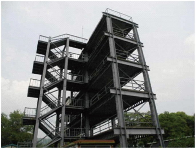
Figure 2. Five-story steel building.

FIGURE 3

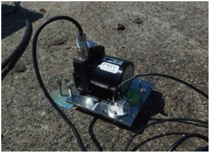
Figure 3. Installation of velocity meter.

FIGURE 4

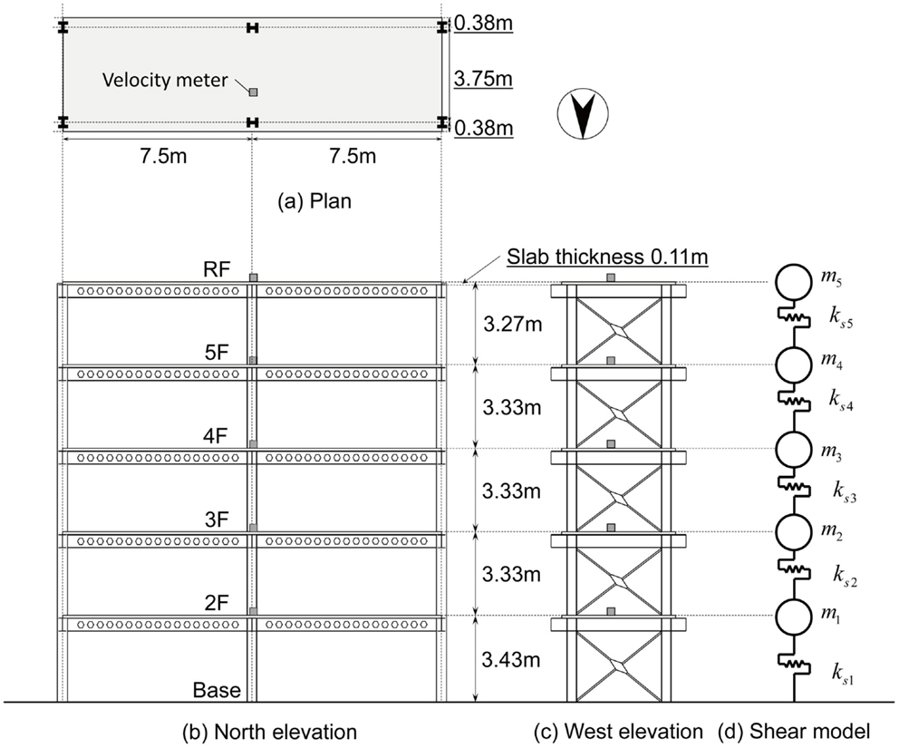
Figure 4. Frame dimension and its shear building model.

TABLE 1

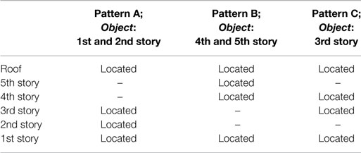
Table 1. Location of velocity meter and measurement pattern for stiffness identification.

Ambient Data Measurement

Figure 5 shows some examples of recorded ambient data at the base, 3rd floor, 4th floor, and roof in the short-span direction in Pattern C. Durations of the measurement time were 5 and 10 min. Figure 6 presents the transfer function of the roof velocity to the base for each pattern of the short-span direction measurements. In Figure 6, the transfer functions evaluated by raw data, i.e., no post-processing, are compared with those after smoothing and filtering. From these preliminary analyses of steel structure, natural frequencies can be estimated as shown in Table 2.

FIGURE 5

Figure 5. Examples of recorded data (ground level, 3rd floor, 4th floor, and roof).

FIGURE 6

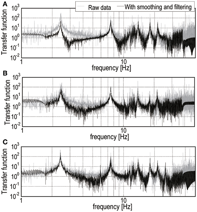
Figure 6. Transfer function of short-span (A) Pattern A, (B) Pattern B, and (C) Pattern C.

TABLE 2

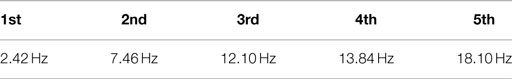
Table 2. Estimated natural frequencies in short-span direction from transfer function (roof/base).

Optimal Combination of Order of ARX Model and Filtering Parameters

Determination of Identification Parameters by Iterative Manipulation

As seen in Figure 6, the transfer functions evaluated by raw data exhibit large variability in the low frequency range. For this reason, it is difficult to obtain the limit value of the identification function directly from the raw data. It is well known that the order of ARX models is important to obtain reliable identification results. Furthermore, it is also observed that the band-pass filter as post-data processing stabilizes the variability of the ARX modeling. Taking these unknown parameters for the structural identification into account, it is needed to investigate the influence of the combination of these unknown parameters on the stability of the identification results.

One of the solutions to this problem, i.e., the identification method combining the previous method (Hernandez-Garcia et al., 2010b; Xing and Mita, 2012) with the band-pass filtering and the ARX modeling is presented here. Figure 7 shows the outline of the identification procedure including the band-pass filtering and the ARX modeling. In the flowchart (Figure 7), three procedures are needed; Procedure 1 is for determination of the order of the ARX model, which was derived by the parametrical analysis to minimize objective functions defined by Eqs (19) and (21); procedure 2 is for determination of the lower cut-off frequency; and procedure 3 is for that of the upper cut-off frequency. Finally, the story stiffnesses are evaluated from the limit value of the identification function in Eq. (4) by selecting unknown identification parameters. If the stability of the limit value is not acceptable, it is needed to select the order of ARX models again in procedure 1. Figure 8 presents examples of SI by using the measured ambient data of the real structure. The red lines, which can be derived by iterative manipulations, are the finally selected identification parameters for the order of the ARX model and cut-off frequencies. However, as seen in Figure 8, the objective functions in terms of these identification parameters vary drastically. Therefore, these procedures of iterative flows to determine several identification parameters may depend on the knowledge of structural engineers so as to derive reliable identification results.

FIGURE 7

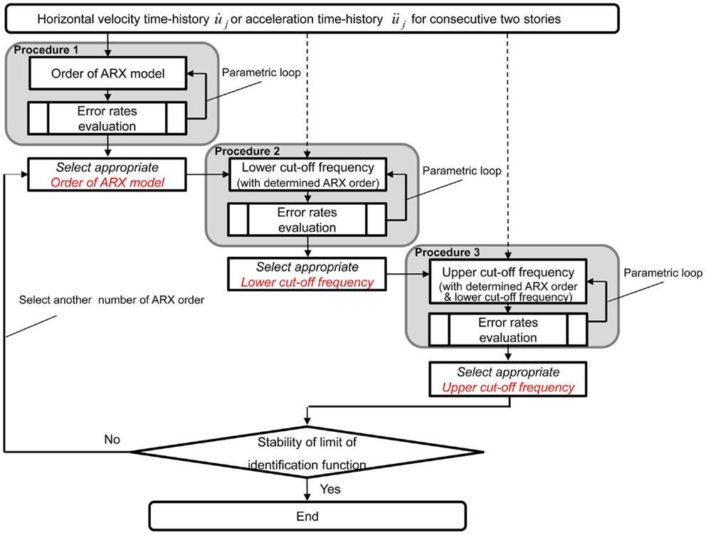
Figure 7. Flowchart of system identification.

FIGURE 8

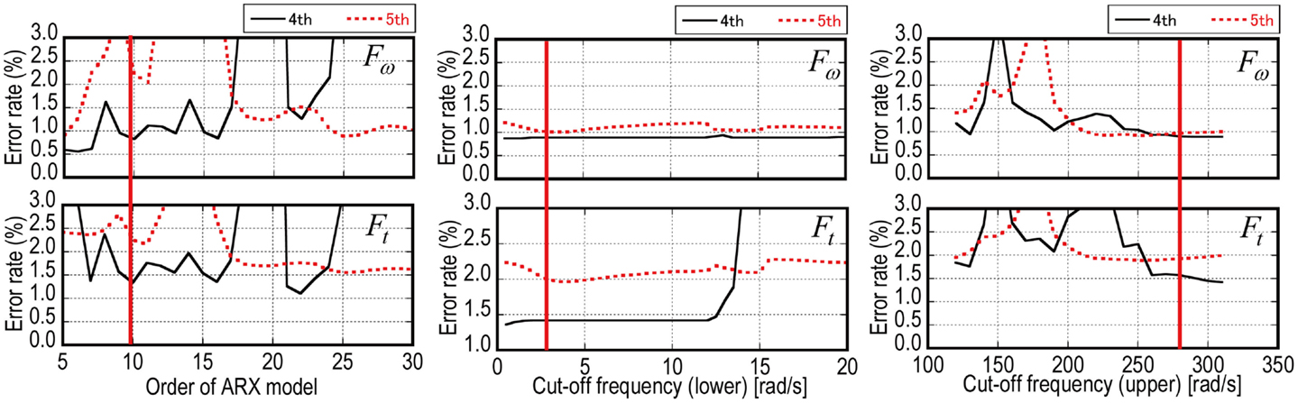
Figure 8. Determination of order of ARX model and cut-off frequencies.

Determination of Identification Parameters by Multi-Objective Optimization

It is important to select an appropriate combination of identification parameters for reliable identification of the story stiffnesses. In this section, this combination will be derived by applying a multi-objective optimization solver based on genetic algorithm. The design parameters for optimization are the order of the ARX model, lower and upper bounds of cut-off frequency. The objective functions are given by Eqs (18) and (20). In the application to the measured ambient data as shown in the following section, four velocity sensors are used simultaneously, which means that the transfer functions and identification functions can be evaluated at three different consecutive stories. For the application to this experimental data, the number of the objective functions in the multi-objective optimization algorithm is six, i.e., the error rate in time domain and frequency domain at three consecutive stories.

The multi-objective optimization algorithm (MOGA-II) implemented in modeFRONTIER 4.5 (ESTECO) is used to investigate the optimal combination of the identification parameters. Initial design parameters are provided by the uniform random number method. Figure 9 describes the multi-dimensional analysis in the post-data processing for all individuals in the multi-objective optimization (the number of designs is 8000). The points connected by lines represent a generated design and the corresponding error rates of objective functions. From this figure, an excellent combination of the identification parameters can be derived by determining an allowable range of objective functions. Figure 9 shows two results (top and bottom illustrations) for different allowable ranges of the objective functions. In the bottom illustration, the error rate in time domain is widen, which causes the wide variability of design parameters. As for the order of ARX models, two different ranges of ARX order can be seen as 26–36 and 58–60 by widening the error rate in time domain. From this multi-dimensional analysis, the evaluation of the objective functions influences the decision making on the identification parameters. Figure 10 shows the comparison of the transfer function (roof/base) obtained from raw data with the transfer functions derived by the optimal combination of the order of ARX models and the cut-off frequencies in the multi-objective optimization (nine combinations are selected here). In Figure 10, no difference can be seen in these combinations, which demonstrates the reliability of the evaluation of error rate in the multi-objective optimization procedure.

FIGURE 9

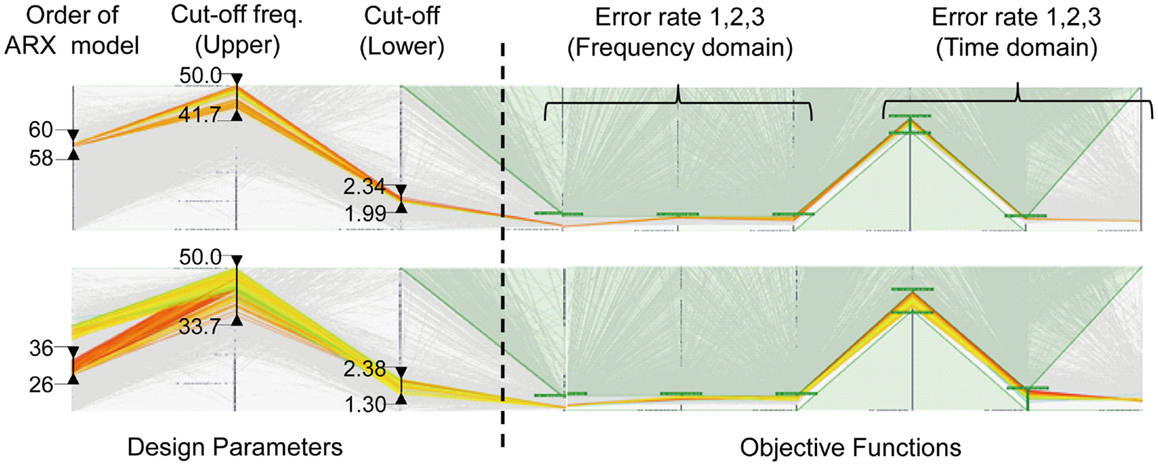
Figure 9. Multi-dimensional analysis for optimal combination of identification parameters.

FIGURE 10

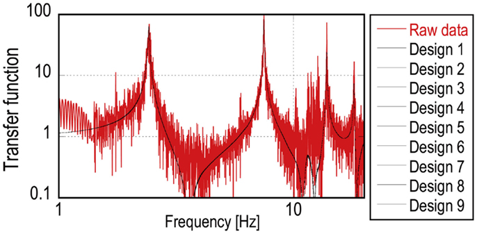
Figure 10. Comparison of transfer functions (raw data VS ARX model).

Stability of Stiffness Identification by Limit Value of Identification Function

By applying the multi-objective optimization algorithm, several designs of the combination of identification parameters are obtained, which can make the objective functions in time and frequency-domain minimized in an acceptable manner. In this section, stability of the story stiffnesses is investigated by applying the SI method to the various (and optimized) identification functions derived by the multi-objective optimization. As explained before, the present SI method needs the evaluation of the limit value of identification functions. In the previously proposed SI method in the same framework, this limit value was just determined by selecting the raw value of the identification function at ω ≈ 0 (called Method 1). In this sense, Method 1 is a simple and primitive one. Figure 11 shows the cumulative frequency of the identified story stiffness k_i (i = 1, 2, …, 5) for various combinations derived from the multi-dimensional analysis in Figure 9 where the number of optimal designs is about 150. It can be observed that identified story stiffnesses by Method 1 have large variability although the selected combination groups of the identification functions are similar. This means instability of the story stiffness identification.

FIGURE 11

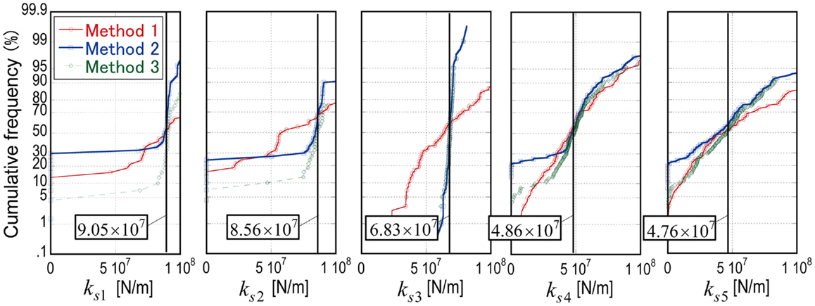
Figure 11. Cumulative frequency of identified story stiffnesses.

For enhancing the stability of story stiffness identification, other approaches to limit value evaluation are proposed as:

Method 2: Using gradient sensitivity of identification function.

Method 3: Using model pole derived by ARX model.

A conceptual illustration of these methods for limit value evaluation is shown in Figure 12. In Method 2, the gradient sensitivity of the identification function is evaluated successively in the frequency domain. The limit of the identification function is determined by evaluating the mean value of the identification functions in a stable range where the gradient of the identification function is sufficiently small (see Figure12: Method 2). While, in Method 3, a raw value of the identification function at a particular frequency determined by the frequency for the model pole of ARX model is used as the limit value of the identification function. The particular frequency point is given by assuming an appropriate constant value, e.g., 0.5, as the ratio to the model pole frequency (see Figure12: Method 3). Let us see Figure 11 again where the cumulative frequency of story stiffnesses is evaluated by the proposed methods. The variability of the identified story stiffnesses can be evaluated from the comparison of the gradient in the cumulative frequency shown in Figure 11. As for the first, second, and third stories, identified story stiffnesses have smaller variability compared with those by Method 1. However, improvement of stability for the fourth and fifth story stiffnesses cannot be observed even in applying Method 2 and 3. This means that it is difficult to determine story stiffnesses in these cases. This instability needs further investigation on the relationship between the objective functions, Eqs (19) and (21), and the identification function derived by the ARX model. Tables 3 and 4 summarize the identified story stiffnesses and natural frequencies obtained by the shear model using the identified story stiffnesses. The identified story stiffnesses derived by Method 2, 3 in Table 3 are determined by the mean values of the selected optimal designs in Figure 11. In Table 3, a frame analysis was conducted by using a frame model including measured section size of columns and beams. It should be mentioned that the boundary condition of the numerical frame analysis may not correspond to the real structure. It is difficult to define “reference stiffness values” because a real building structure cannot be expressed by a shear building model exactly.

FIGURE 12

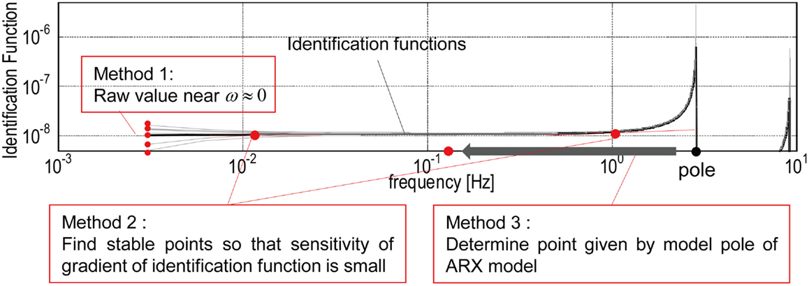
Figure 12. Limit value evaluation for identification functions derived by ARX model.

TABLE 3

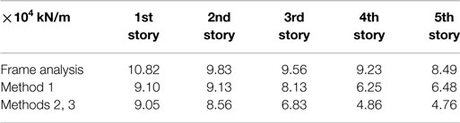
Table 3. Identified story stiffness.

TABLE 4

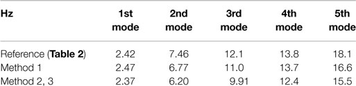
Table 4. Natural frequencies of identified shear model.

Conclusion

A previously proposed story-wise stiffness identification method using an ARX model for a shear building structure has been applied to the case where the shear building is subjected to micro-tremors measured in a full-scale steel frame structure. While earthquake ground motions and the building responses to such inputs are necessary in the previous method, it has been shown that micro-tremors can be used for identification within the same framework. This enhanced the usability of the previously proposed identification method. The difficulty in the selection of the combination of identification parameters, i.e., the order of the ARX model and the cut-off frequencies of band-pass filtering, has been tackled by a multi-objective optimization algorithm. Advantageous features are as follows:

(1) Micro-tremors can be used as an input for the previously proposed SI method for shear building models regardless of its small vibration level.

(2) In order to investigate identification parameters for reliable identification based on the ambient vibration, the objective functions in time and frequency domains have been proposed by applying filtering in the frequency range (low and high cuts) and averaging in time domain (sequential time-window shift for Fourier transformation and averaging).

(3) Stability in the story stiffness evaluation for optimal combinations of identification parameters derived by the multi-objective optimization has been compared among various limit-value estimation approaches. It has been observed that the limit value by selecting the raw value of the identification function at ω ≈ 0 is not necessarily appropriate. Proposed approaches such as using gradient sensitivity of the identification function or the model pole of the ARX model make it stable to derive story stiffnesses.

Conflict of Interest Statement

The authors declare that the research was conducted in the absence of any commercial or financial relationships that could be construed as a potential conflict of interest.

Acknowledgements

This research is partly supported by the Grant-in-Aid for Scientific Research (No. 24246095) in Japan. This support is gratefully acknowledged.

References

Adachi, S. (2009). Fundamentals of System Identification. Tokyo: Denki University Press.

Google Scholar

Agbabian, M. S., Masri, S. F., Miller, R. K., and Caughey, T. K. (1991). System identification approach to detection of structural changes. ASCE J. Eng. Mech. 117, 370–390. doi: 10.1061/(ASCE)0733-9399(1991)117:2(370)

CrossRef Full Text | Google Scholar

Barroso, L. R., and Rodriguez, R. (2004). Damage detection utilizing the damage index method to a benchmark structure. ASCE J. Eng. Mech. 130, 142–151. doi:10.1061/(ASCE)0733-9399(2004)130:2(142)

CrossRef Full Text | Google Scholar

Beck, J. L., and Jennings, P. C. (1980). Structural identification using linear models and earthquake records. Earthquake Eng. Struct. Dyn. 8, 145–160. doi:10.1002/eqe.4290080205

CrossRef Full Text | Google Scholar

Doebling, S. W., Farrar, C. R., Prime, M. B., and Shevitz, D. W. (1996). Damage Identification and Health Monitoring of Structural and Mechanical Systems from Changes in their Vibration Characteristics: a Literature Review. Report LA-13070-MS. Los Alamos National Laboratory, Los Alamos.

Google Scholar

Fujino, Y., Nishitani, A., and Mita, A. (2010). Proceedings of 5th World Conference on Structural Control and Monitoring (5WCSCM). Tokyo.

Google Scholar

Fujita, K., Ikeda, A., Shirono, M., and Takewaki, I. (2013). System identification of high-rise buildings using shear-bending model and ARX model: experimental investigation. Proc. of ASEM13(ICEAS13), 2803–2815.

Google Scholar

Ghanem, R., and Shinozuka, M. (1995). Structural-system identification I: theory. ASCE J. Eng. Mech. 121, 255–264. doi:10.1061/(ASCE)0733-9399(1995)121:2(255)

CrossRef Full Text | Google Scholar

Hart, G. C., and Yao, J. T. P. (1977). System identification in structural dynamics. ASCE J. Eng. Mech. Div. 103, 1089–1104.

Google Scholar

Hernandez-Garcia, M. R., Masri, S. F., Ghanem, R., Figueiredo, E., and Farrar, C. R. (2010a). An experimental investigation of change detection in uncertain chain-like systems. J. Sound Vib. 329, 2395–2409. doi:10.1016/j.jsv.2009.12.024

CrossRef Full Text | Google Scholar

Hernandez-Garcia, M., Masri, S. F., Ghanem, R., Figueiredo, E., and Farrar, R. A. (2010b). A structural decomposition approach for detecting, locating, and quantifying nonlinearities in chain-like systems. Struct. Control Health Monit. 17, 761–777. doi:10.1002/stc.396

CrossRef Full Text | Google Scholar

Hjelmstad, K. D. (1996). On the uniqueness of modal parameter estimation. J. Sound Vib. 192, 581–598. doi:10.1006/jsvi.1996.0205

CrossRef Full Text | Google Scholar

Hjelmstad, K. D., Banan, Mo.R., and Banan, Ma.R. (1995). On building finite element models of structures from modal response. Earthquake Eng. Struct. Dyn. 24, 53–67. doi:10.1002/eqe.4290240105

CrossRef Full Text | Google Scholar

Hoshiya, M., and Saito, E. (1984). Structural identification by extended Kalman filter. ASCE J. Eng. Mech. 110, 1757–1770. doi:10.1061/(ASCE)0733-9399(1984)110:12(1757)

CrossRef Full Text | Google Scholar

Housner, G., et al. (1997). Special issue, structural control: past, present, and future. ASCE J. Eng. Mech. 123, 897–971. doi:10.1061/(ASCE)0733-9399(1997)123:9(897)

CrossRef Full Text | Google Scholar

Ji, X., Fenves, G. L., Kajiwara, K., and Nakashima, M. (2011). Seismic damage detection of a full-scale shaking table test structure. ASCE J. Struct. Eng. 137, 14–21. doi:10.1061/(ASCE)ST.1943-541X.0000278

CrossRef Full Text | Google Scholar

Johnson, E., and Smyth, A. (eds) (2006). Proceedings of 4th World Conference on Structural Control and Monitoring (4WCSCM). San Diego, CA: IASC.

Google Scholar

Kobori, T., Seto, Y. K., Iemura, H., and Nishitani, A. (eds) (1998). Proceedings of 2nd World Conference on Structural Control. Kyoto: John Wiley & Sons.

Google Scholar

Koh, C. G., See, L. M., and Balendra, T. (1991). Estimation of structural parameters in time domain: a substructure approach. Earthquake Eng. Struct. Dyn. 20, 787–801. doi:10.1002/eqe.4290200806

CrossRef Full Text | Google Scholar

Kozin, F., and Natke, H. G. (1986). System identification techniques. Struct. Saf. 3, 269–316. doi:10.1016/0167-4730(86)90006-8

CrossRef Full Text | Google Scholar

Maeda, T., Yoshitomi, S., and Takewaki, I. (2011). Stiffness-damping identification of buildings using limited earthquake records and ARX model. J. Struct. Construct. Eng., Architectural Inst. of Japan 666, 1415–1423. doi:10.3130/aijs.76.1415

CrossRef Full Text | Google Scholar

Masri, S. F., Nakamura, M., Chassiakos, A. G., and Caughey, T. K. (1996). A neural network approach to the detection of changes in structural parameters. ASCE. J. Eng. Mech. 122, 350–360. doi:10.1061/(ASCE)0733-9399(1996)122:4(350)

CrossRef Full Text | Google Scholar

Minami, Y., Yoshitomi, S., and Takewaki, I. (2013). System identification of super high-rise buildings using limited vibration data during the 2011 Tohoku (Japan) earthquake. Struct. Control Health Monit. 20, 1317–1338. doi:10.1002/stc.1537

CrossRef Full Text | Google Scholar

Nagarajaiah, S., and Basu, B. (2009). Output only modal identification and structural damage detection using time frequency & wavelet techniques. Earthquake Eng. Eng. Vib. 8, 583–605. doi:10.1007/s11803-009-9120-6

CrossRef Full Text | Google Scholar

Shinozuka, M., and Ghanem, R. (1995). Structural-system identification II: experimental verification. ASCE J. Eng. Mech. 121, 265–273. doi:10.1061/(ASCE)0733-9399(1995)121:2(265)

CrossRef Full Text | Google Scholar

Takewaki, I., and Nakamura, M. (2000). Stiffness-damping simultaneous identification using limited earthquake records. Earthquake Eng. Struct. Dyn. 29, 1219–1238. doi:10.1002/1096-9845(200008)29:8<1219::AID-EQE968>3.0.CO;2-X

CrossRef Full Text | Google Scholar

Takewaki, I., and Nakamura, M. (2005). Stiffness-damping simultaneous identification under limited observation. ASCE J. Eng. Mech. 131, 1027–1035. doi:10.1061/(ASCE)0733-9399(2005)131:10(1027)

CrossRef Full Text | Google Scholar

Takewaki, I., and Nakamura, M. (2009). Temporal variation of modal properties of a base-isolated building during an earthquake. J. Zhejiang Univ. Sci. A 11, 1–8. doi:10.1631/jzus.A0900462

CrossRef Full Text | Google Scholar

Udwadia, F. E., Sharma, D. K., and Shah, P. C. (1978). Uniqueness of damping and stiffness distributions in the identification of soil and structural systems. ASME J. Appl. Mech. 45, 181–187. doi:10.1115/1.3424224

CrossRef Full Text | Google Scholar

Xing, Z., and Mita, A. (2012). A substructure approach to local damage detection of shear structure. Struct. Control Health Monit. 19, 309–318. doi:10.1002/stc.439

CrossRef Full Text | Google Scholar

Zhang, D. Y., and Johnson, E. A. (2013). Substructure identification for shear structures with nonstationary structural responses. ASCE J Eng Mech. 139, 1769–1779. doi:10.1061/(ASCE)EM.1943-7889.0000626

CrossRef Full Text | Google Scholar

Appendix: ARX Model

Let k denote a discrete time step number (Adachi, 2009). When the output, the input, and white noise are denoted by y(⋅), u(⋅), and w(⋅), the ARX model is described by:

$\begin{array}{l}\hfill y\left(k\right)+a_{1}y\left(k-1\right)+\cdots +a_{n_a}y\left(k-n_a\right)=b_{1}u\left(k-1\right)+\cdots +b_{n_b}u\left(k-n_b\right)+w\left(k\right)\end{array}$ (A1)

The transfer function can be expressed in terms of the shift operator q.

$G\left(q\right)=\mathrm{B}\left(q\right)∕A\left(q\right)$ (A2)

where

$\text{A}\left(q\right)=1+a_1{q}^{-1}+\cdots +a_{n_a}{q}^{-n_a},$ (A3)

$\text{B}\left(q\right)=b_1{q}^{-1}+\cdots +b_{n_b}{q}^{-n_b}$ (A4)

The relation between the Z transformation and the Fourier transformation is given by Eq. (A5) and the transfer function in terms of the variable q in Eq. (A2) can be expressed as the transfer function in terms of the variable ω (circular frequency). In Eq. (A6), T₀ denotes the sampling period.

$q=e^{\mathrm{i}\mathrm{\omega }{T}_0}$ (A5)

$G\left(\mathrm{\omega }\right)=\frac{b_1{e}^{-\mathrm{i}\mathrm{\omega }{T}_0}+\cdots +b_n{e}^{-\mathrm{i}n\mathrm{\omega }{T}_0}}{1+a_1{e}^{-\mathrm{i}\mathrm{\omega }{T}_0}+\cdots +a_n{e}^{-\mathrm{i}n\mathrm{\omega }{T}_0}}$ (A6)

Define the parameter vector θ and the data vector φ(k) by Eqs (A7) and (A8), respectively. The prediction of the output at time k from the input–output data until the time number (k − 1) can be expressed by Eq. (A9).

$\theta ={\{a_1\cdots a_{n_a}{b}_1\cdots b_{n_b}\}}^T$ (A7)

$\phi (k)=\{-y(k-1)\cdots -y{(k-n_a)}^{T}u(k-1)\cdots u(k-n_b)\}$ (A8)

$\widehat{y}\left(k;\mathrm{\theta }\right)={\mathrm{\theta }}^T\mathrm{\phi }\left(k\right)$ (A9)

Using Eq. (A9), the prediction error in the ARX model can be described by:

$\mathrm{\epsilon }\left(k,\mathrm{\theta }\right)=y\left(k\right)-\widehat{y}\left(k;\mathrm{\theta }\right)=y\left(k\right)-{\mathrm{\theta }}^T\mathrm{\phi }\left(k\right)$ (A10)

Introduce the objective function by Eq. (A12) for predicting the parameter vector θ. Then the least-squares method can be applied to the parameter prediction problem.

$J_N\left(\mathrm{\theta }\right)=\frac{1}{N_d}{\displaystyle \sum _{k=1}^{N_d}{\epsilon }^2(k;\theta )}$ (A11)

In this case, the prediction problem of θ can be reduced to the following simultaneous equations.

$\mathbf{\text{R}}\mathrm{\theta }=\mathbf{\text{f}}$ (A12)

where

$\mathbf{\text{R}}=\frac{1}{N_d}\mathrm{\Phi }{\mathrm{\Phi }}^T\left(\mathrm{\Phi }={\left[\begin{array}{cccc}\hfill \mathrm{\phi }\left(1\right)\hfill & \hfill \mathrm{\phi }\left(2\right)\hfill & \hfill \cdots \hfill & \hfill \mathrm{\phi }\left(N_d\right)\hfill \\ \hfill \hfill \end{array}\right]}^T\right)$ (A13)

$\text{f}=\frac{1}{N_d}{\mathbf{\Phi }}^T\text{y\hspace{1em}}\left(y={\{y(1)y(2)\cdots y(N_d)\}}^T\right)$ (A14)

The least-square estimation of the unknown parameters based on the N_d-pair input–output measured data may then be expressed by:

$\widehat{\mathrm{\theta }}={\mathbf{\text{R}}}^{-1}\mathbf{\text{f}}$ (A15)