Predicting Topographic Effect Multipliers in Complex Terrain With Shallow Neural Networks

Introduction

Prediction of wind speed in complex topography is integral to the design and operation of civil infrastructure (e.g., Baker et al., 1985; Huang and Xu, 2013; Ngo and Letchford, 2009), siting and optimization of wind energy resources (Barthelmie et al., 2009; Badger et al., 2014; Wilczak et al., 2015; Brahimi, 2019; Haupt et al., 2019; Olson et al., 2019; Santoni et al., 2020), forest management (e.g., Quill et al., 2020), and meteorological forecasting (e.g., Finnigan et al., 2020; Donadio et al., 2021). Within the context of wind loads on structures, surface gusts occurring in a flat expanse can double in magnitude upslope (Kondo et al., 2002), quadrupling the loads occurring on low-rise buildings. Therefore, modern wind load provisions (e.g., ASCE 7–16) account for the presence of hills, escarpments, and other topographic features through provisioning of rational engineering analysis for simple landforms or special wind region maps for areas that have complex topography. Additional methods to account for complex terrain in structural design include wind tunnel testing and computational fluid dynamics (CFD) simulation. While over time CFD will likely become the dominant method to predict speedup, these methods are still computationally expensive, time intensive, and occasionally prone to not resolving flows in complex terrain well. Thus, this study explores the use of shallow neural networks, which are excellent universal function approximators when trained properly (Hornik et al., 1989).

Flow over isolated topographic features has been studied for decades (e.g., Taylor and Teunissen, 1987; Salmon et al., 1998), later extending to the study of complex landforms (e.g., Chock and Cochran, 2005; Rasouli et al., 2009; Kikuchi and Ishihara, 2012; McAuliffe and Larose, 2012; Lange, 2016). The present research adds to the body of work that uses data-driven methods to predict speedup, using six mountainous regions in mainland Puerto Rico and the municipal islands of Vieques and Culebra as the study testbed (Figure 1). Multiple shallow neural network configurations are applied to surface velocity measurements obtained from boundary layer wind tunnel (BLWT) modeling of complex terrain, including coastal-to-mountain transitions and inner mountain ranges. The results support the efficacy of this approach for rapid and computationally inexpensive prediction of wind speedup in complex topography using digital elevation model (DEM) data. We conclude that BLWT topographic modeling data obtained from different facilities should be warehoused in a single, openly accessible data atlas to validate, improve, and cross-compare the results of predictive models for a wide range of terrain and land cover types.

FIGURE 1

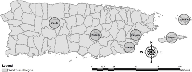
FIGURE 1. Regions of Puerto Rico selected for testing at BLWT at UF.

Motivating the study is the impact of Hurricane Maria (2017), which struck the island as a Saffir Simpson Hurricane Wind Scale Category 4 storm that caused more than 4,000 deaths (Kishore et al., 2018), $90B in economic loss (Pasch et al., 2019), and widespread power outages that occurred for more than 6 months (Kwasinski et al., 2019). The National Hurricane Center (Pasch et al., 2019) speculated that “winds of category 5 intensity were almost certainly felt at some elevated locations on the island,” which was further evidenced by post-storm damage assessments led by the FEMA Mitigation Assessment Team (Bass et al., 2018) and Prevatt et al. (2018). The testbed encompasses many of the most heavily impacted areas, as data were collected at the request of the FEMA Building Science Branch for the development of a special wind region map that was later adopted by the 2018 Puerto Rico Construction Code. The selection of these six regions during this study considered Hurricane Maria’s path, location of urban areas, and terrain complexity parameters (i.e., elevation, slope, curvature, and rugosity) calculated using ArcGIS and DEM Surface Tools for ArcGIS (Jenness, 2013). Table 1 lists the corresponding range of values for elevation, slope, curvature, and rugosity. Data collected for this project are available for download at the National Science Foundation Natural Hazards Engineering Research Infrastructure (NHERI) DesignSafe site (www.designsafe-ci.org).¹

TABLE 1

TABLE 1. Terrain complexity parameters.

Background

Definition of Wind Speedup and Topographic Effect Multipliers

For structural design, topographic wind speedup effects are typically quantified as a non-dimensional multiplier that amplifies the velocity pressure used in the calculation of localized wind loads on the building’s surface. Ngo and Letchford (2009) provide an overview of four such codified procedures from four internationally recognized building codes. As shown in Figure 2, the structural load multipliers are derived from a ratio that relates the gust wind speed (${\widehat{u}}_{zt}$) at elevation z above the site of interest to the gust wind speed (${\widehat{u}}_z$) occurring in a flat expanse under the same wind conditions. This ratio is termed the topographic effect multiplier ($M_{zt}$), which is equivalent to 1 + the fractional speedup ratio ($\Delta {\widehat{u}}_z/{\widehat{u}}_z$) given elsewhere in the literature.

$M_{zt}=\frac{{\widehat{u}}_{zt}}{{\widehat{u}}_z}=\frac{{\widehat{u}}_z+\Delta {\widehat{u}}_z}{{\widehat{u}}_z}=1+\frac{\Delta {\widehat{u}}_z}{{\widehat{u}}_z}(1)$

FIGURE 2

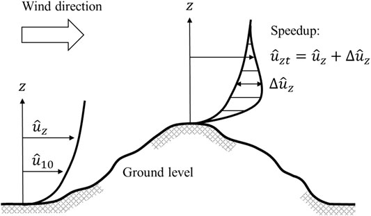
FIGURE 2. Topographic wind speedup.

Methods to Predict Topographic Wind Speedup in Strong Winds

Approaches to predict topographic wind speedup include analytical methods (e.g., Jackson and Hunt, 1975; Deaves, 1980), physical simulation through boundary layer wind tunnel modeling (e.g., Glanville and Kwok, 1997; Chock and Cochran, 2005; Lubitz and White, 2007; Rasouli et al., 2009; Kikuchi and Ishihara, 2012; McAuliffe and Larose, 2012; Lange, 2016), and CFD (e.g., Abdi and Bitsuamlak, 2014). The two physical simulation efforts most relevant to this study are Chock and Cochran (2005) and McAuliffe and Larose (2012). Chock and Cochran (2005) conducted a “microzonation” study to predict windspeed up factors for use in wind load provisioning for the Hawaiian Islands by applying linear regression to hot film anemometer measurements taken over a 1:6000 scale model of Oahu and its corresponding DEM data. The current study adopts a similar approach; however, it applies a neural network (i.e., logistic regression) for prediction. McAuliffe and Larose (2012) modeled a wind farm at 1:1500 scale to study aerodynamic scaling effects; its experimental design heavily informed the current study.

Finnigan et al. (2020) provides a historical narrative on the development of analytical and numerical methods and supporting experiments in BLWTs and in the field, e.g., Askervein Hill (Taylor and Teunissen, 1987) and Perdigão (Mann et al., 2017). Here we turn to describing recent applications of machine learning approaches to improve wind speed prediction.

In the last two decades, artificial neural networks have found a broad range of applications in the study of boundary layer flows. Selected examples include the design and operation of wind tunnels (e.g., Križan et al., 2015), prediction of design wind speeds for civil infrastructure (e.g., Huang and Xu, 2013), and forecasting for wind energy resources (e.g., Burlando and Meissner, 2017; Chen et al., 2018; Liu et al., 2018; Yu et al., 2018; Brahimi, 2019). Starting in the 2000s, machine learning began to be applied in the prediction of topographic wind speedup. One of the first studies was led by Bitsuamlak et al. (2002), who successfully trained a model to predict speedup over shallow and steep sinusoidal hills to match analytical modeling. Bitsuamlak et al. (2007) subsequently incorporated CFD data to quantify speedup accounting for surface roughness conditions. Robert et al. (2012) produced monthly wind speed maps from a data architecture that include multiscale topographic features extracted from a digital elevation model and weather station data. Burlando and Meissner (2017) and Mayo et al. (2018) developed hybrid approaches involving CFD, numerical weather prediction (NWP), and surface wind measurements to inform neural network modeling. More recently, Donadio et al. (2021) developed a highly automated “prediction pipeline” that integrated global and regional NWP to predict wind speed and wind energy production.

These studies foretell of a promising future for regional-scale modeling of wind speedup in complex terrain accounting for the influence of wind directionality or by extension, local climatology. The current work continues to assess the premise that wind speedup in adiabatic boundary layer flow conditions can be predicted directly from elevation data, within the experimental limitations imposed by conducting geometrically scaled physical simulations in a BLWT. The work presented uses data collected over scaled models of complex terrain regions, to develop a feed forward neural network architecture. The literature review provides a summary of the efforts to implement neural networks for wind speed prediction, but no attempt has been made to train a neural network with the goal of predicting topographic wind speedup multipliers over real complex terrain.

Methodology

Physical Simulations in the Boundary Layer Wind Tunnel

Development Section Configuration, Instrumentation, and Approach Flow Conditions

Experiments were carried out in the BLWT located at the Powell Family Structures and Materials Laboratory at the University of Florida. Catarelli et al. (2020) describes the tunnel’s operating characteristics and flow simulation capabilities. Refer to Figure 3 for details on the BLWT configuration used during testing. In this study, the roughness elements in the “Terraformer” development section were oriented in the wide configuration to a uniform height of h = 7 mm or 20 mm to produce marine and suburban aerodynamic roughness lengths of $z_0$ = 0.005 and 0.300 m full-scale (FS) at a geometric scale of 1:3100, respectively. At the chosen geometric scale of 1:3100, matching z₀ to achieve the desired mean velocity profiles effected a reduction in the longitudinal turbulence intensity for the rougher case from an expected value of 25% to nominally 15%. Models were installed in a 4 m turntable that was rotated in one of 16 wind directions (N, NNE, … , NNW). The exposure was selected based on the specific upwind terrain of the model section being tested.

FIGURE 3

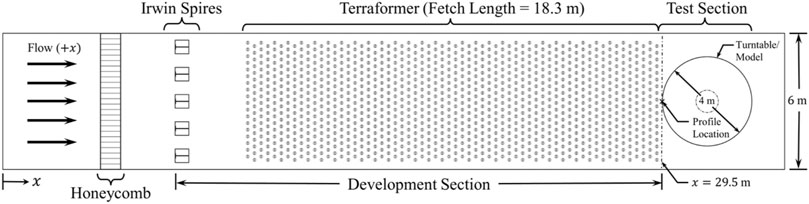
FIGURE 3. Boundary Layer Wind Tunnel Configuration.

Turbulent Flow Instrumentation (TFI) Cobra Probes measured three components of velocity with a sampling frequency of 1250 Hz. Figure 4A shows the dimensions of the probe, which controlled how close to the surface measurements could be made without interfering with the flow. The lowest elevation that could be achieved without introducing speedup between the probe and the model was determined to be approximately three probe head diameters (∼8 mm above the tunnel floor or 25 m at full scale). An automated gantry system (Figure 4B) translated the probes laterally, vertically, and longitudinally using a user-defined sample location input file. Data were then filtered using a 3^rd order Butterworth filter with a 150 Hz cutoff frequency.

FIGURE 4

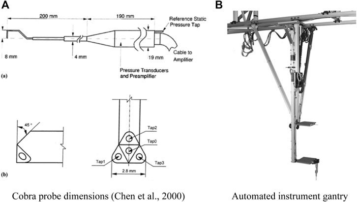
FIGURE 4. Cobra probe instrumentation. (A) Cobra probe dimensions (Chen et al., 2000). (B) Automated instrument gantry.

Gust values were quantified to conservatively estimate the surface wind field intensity. Given the complex flow conditions, the gust value was obtained from a moving average of the instantaneous wind speed magnitude (s) of the three-dimensional wind speed magnitude (i.e., $s=\sqrt{u^2+v^2+w^2}$ where the velocity components are defined as u = longitudinal, v = lateral, and w = vertical) instead of the longitudinal component to ensure that the scalar wind speed maxima was enveloped in the result. Second, the gust was computed as $\widehat{s}=S+g{\sigma }_s$, where S and ${\sigma }_s$ are the mean and standard deviation of the instantaneous wind speed magnitude, respectively. The peak factor (g) was set to 3.0, which Balderrama et al. (2012) has shown to be a conservative upper bound for strong winds generated by Atlantic tropical cyclones (TC) landfalling in a variety of surface roughness exposures. The selected value of g is based on a T = 600 s duration record because TCs, as a rule, exhibit non-stationary behavior for longer time periods. The value would need to be re-referenced to T = 3,600 s for straight line wind applications.

The automated gantry system and Cobra Probes were also used to measure velocity profiles immediately upwind of the models. Figure 5 presents representative profiles of the longitudinal mean velocity and turbulence intensity for the u, v, and w components. Data measured in the inertial sublayer (ISL) portion of the neutral boundary layer are compared to the logarithmic law modified by Sutton (1949) to account for a zero-plane displacement. Figure 6 presents plots of the longitudinal turbulence spectra measured at the end of the Terraformer in the centerline of the tunnel at heights of $z=$ 8 and 988 mm (i.e., full-scale dimensions of $z$ = 25 and 3,063 m, respectively) after applying Welch’s method (Bendat et al., 2000) to the unfiltered velocity records. Data are compared to the power spectra model in ESDU 74030 and 74031 (1974), which was first derived by von Kármán (1948) for isotropic turbulence:

$n{S}_{uu}(z,n)/{\sigma }_u^2=4f/{\left(1+70.8f^2\right)}^{\frac{5}{6}}(2)$

where $f=n{L}_u^x/U$, $n$ is the frequency, $L_u^x$ is the longitudinal integral length scale of the turbulence, $U$ is the longitudinal mean velocity, $S_{uu}(z,n)$ is the power spectral density function, and ${\sigma }_u$ is the longitudinal standard deviation of velocity. The data exhibit the same phenomenon identified by McAuliffe and Larose (2012) during topographic modeling of a 1:1,500 scale wind farm in Quebec. Similitude in the freestream flow is achieved, however the observed energy at the high frequency range near the surface is larger than the von Kármán model. McAuliffe and Larose (2012) attributed this phenomenon to eddy surface layer behavior, where anisotropic spectral decay proportional to the inverse of the wavenumber ( $k^{-1}$) is expected to occur. Although not the subject of this paper, it does draw attention to the validity of the upper bound of geometric scaling requirements, which is generally accepted as 1:5,000 (ASCE 49, 2012).

FIGURE 5

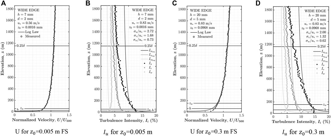
FIGURE 5. Mean velocity and turbulence intensity profiles. (A) U for $z_0$ = 0.005 m FS, (B) $I_u$ for $z_0$ = 0.005 m, (C) U for $z_0$ = 0.3 m FS, and (D) $I_u$ for $z_0$ = 0.3 m.

FIGURE 6

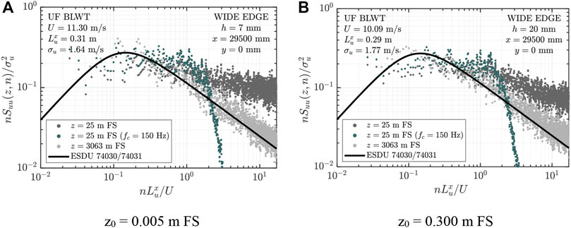
FIGURE 6. Longitudinal power spectra. (A) z₀ = 0.005 m FS. (B) z₀ = 0.300 m FS.

Topographic Models

Six 1:3,100 scale topographic models of 12.4 km diameter circular regions encompassing the municipalities of Aibonito, Culebra Humacao, Utuado, Vieques, and Yabucoa (Figure 1) were constructed from DEM data obtained from the U.S. Geological Survey (USGS). Figure 7A shows the Yabucoa model installed in the BLWT turntable. Data represent the bare-earth surface at a resolution of 1/3 arc-second (∼10 m) referenced to the North American Vertical Datum of 1983 (NAVD83) High Accuracy Reference Network (HARN) State Plane Puerto Rico Virgin Islands Federal Information Processing Standards (FIPS) 5200.

FIGURE 7

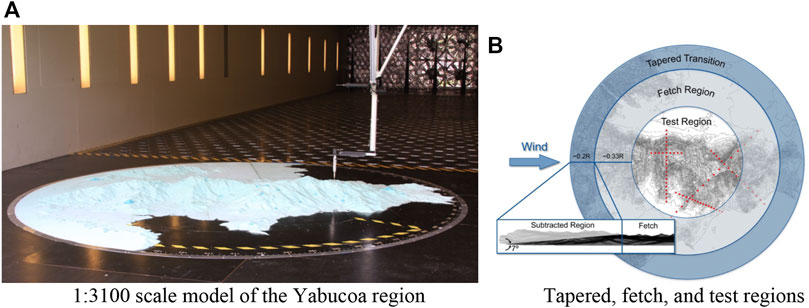
FIGURE 7. Tapered, fetch, test regions and measurement locations of the model. (A) 1:3,100 scale model of the Yabucoa region. (B) Tapered, fetch, and test regions.

A MultiCam APEX304 3-axis computer numerical control (CNC) routing system fabricated the topographic models by cutting contours into Type IV 25 psi XPS foam panels, which were layered to build the final model. A 30 m spatial filter was applied to the DEM data to ensure the CNC could follow the tool paths. The contour interval height was selected from results of trial-and-error testing of a surface flow over model escarpment routed at different cut heights (smooth, 1, 3, and 5 mm) across the width of the tunnel. Dimensions of the model escarpment were 3.0 m W × 0.3 m H × 1.7 m L. The front section of the model was routed into a curved ramp (rotation angle from 0–45° along a circular arc), and the back section was a tabletop configuration. Ultimately the 3 mm height was chosen because coarser routing produced an unrealistic rise in turbulence intensity over the escarpment and using a finer contour would have been time prohibitive given the project schedule.

The outer regions of the models were modified to minimize the effects of the abrupt transitions in flow caused by the truncation of mountainous areas at the edge of the model. As Figure 7B shows, each model was divided into three regions. Measurements were confined to the inner R = 1 m radius (5 km FS) circular region unless the outer region was flat. No modification was made to the annular “fetch” region (nominal width of R/3) surrounding it, ensuring that surface flows would travel at least 2 km full-scale over unmodified terrain before reaching the measurement location. Finally, any terrain projecting above a line angled 7° upward from the outermost model edge at the tunnel floor was excluded, with the angle of the cutting plane having been chosen to prevent boundary layer separation (ANSI (American National Standards Institute), 2007).

Data Collection and Processing

Surface wind speed measurements were obtained for each region (model) from gridded locations for each of 16 wind directions in 30 s duration records. Table 2 provides a measurement (grid location) count for each region, the corresponding number of records that passed quality control, and the minimum and maximum elevations of the measurement locations. Records were rejected if the Cobra Probe failed to collect at least 80% of the record. Sample quality drops if the resultant wind velocity is outside of the 45° cone of acceptance around the probe head. This generally occurs in separated flow regions where topographic speedup effects are not a concern.

TABLE 2

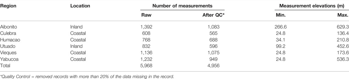
TABLE 2. Directional surface wind measurement on the topographic models.

Measurement locations, shown in Figure 7B, were selected to coincide with lines parallel to the 16 wind compass rose aligned with true north (i.e., N, NNE, … , NNW), with two lines generally intersecting near a local maxima at the terrain and at least one of those lines following the highest ridgeline. Measurement locations extended between 300 and 4,400 m from the local maxima, generally terminating in a valley or a flat expanse. Spacing between locations varied from 100–500 m.

The testing sequence was as follows:

1) The Terraformer height was adjusted to create a compatible upwind fetch condition by setting the roughness element height (h) to

a) h = 20 mm ($z_0$ = 0.300 m) for regions located fully inside a mountain range (e.g, Aibonito, Utuado) and for the case where terrain that extended beyond the model perimeter. This category of fetch is referred to as “rough” because of both the mountainous terrain and treed conditions that were prevalent in these locations

b) h = 7 mm ($z_0$ = 0.005 m) where the model terminated at the floor before the perimeter (i.e., where upwind marine or flat, open conditions were present). This category of fetch is referred to as the “smooth-to-rough transition”

2) The BLWT fans were brought up to maximum operating speed (20 m/s freestream)

3) Reference velocity measurements were obtained at a height of 8 mm (25 m FS) at five locations spaced 750 mm apart at the trailing edge of the Terraformer development section

4) Data were sequentially collected at the model measurement locations at a height of 8 mm (25 m FS) for a 30 s duration

5) Fan speed was reduced to 0 RPM

6) The turntable was rotated 22.5° to the next wind direction

7) Steps 1–6 were repeated until all 16 wind directions were tested

8) Steps 1–7 were repeated until all six models were tested.

Artificial Neural Networks

Single and double hidden layer shallow feedforward neural networks were constructed using the Deep Learning Toolbox in Matlab 2019a. The model architectures consisted of neurons initialized with random weights and biases. Figure 8 shows the generic single layer neural network architecture configuration used. Hidden layers were fully connected using rectifying linear unit activation functions, and the output layer used a linear activation function. The Levenberg-Marquardt training method (Hagan and Menhaj, 1994) was applied following Liu (2010) to optimize the weights and biases based on the mean square error. During training, the network was limited to only 1,000 epochs and six validation checks to avoid overfitting the data. Data were separated 70% for training, 15% for testing, and 15% for validation at the beginning of each training process via random assignment. The 4,956 quality-controlled records (Table 2) measured from 373 unique geographic locations in 16 wind directions were used to train the neural network.

FIGURE 8

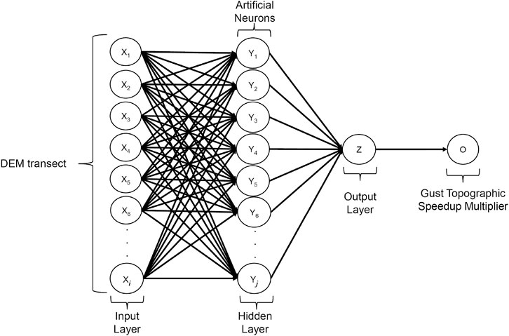
FIGURE 8. Single Layer Network Architecture.

The model input consisted of 2 km of upwind terrain elevation data and 1 km of downwind terrain elevation data at each site in each wind direction. The input was chosen after comparing results of training for different combinations of inputs that included elevation and slope. Inputting the slope as the single variable (as was done in Chock and Cochran, 2005) was also attempted. None of these inputs produced a better trained model than inputting the elevation data alone.

The model output was the gust topographic effect multiplier at each site in each wind direction. As discussed in the Methodology, the choice of calibrating the approach flow to match the mean velocity profile led to a reduction in turbulence intensity for the rough terrain case, leading to the turbulence intensity characteristics representative of open exposure fetch. Given that the M_zt values are based on gusts (usually referenced to open exposure), the reference values were not adjusted for this comparison.

Results

Sensitivity analyses were conducted on multiple configurations of shallow neural networks. Figures 9, 10 present results for single and double hidden layer network configurations, respectively. The number of neurons was parametrically increased from 10 to 150 neurons for the single hidden layers and 10 to 80 neurons for the double hidden layers, in steps of 20 neurons. Fine (10 m) and coarse (100 m) horizontal DEM input resolutions were evaluated separately for each network. Results are stratified by the upwind terrain (smooth-to-rough transition, rough) and horizontal fetch resolution. The box and whisker markers characterize coefficients of determination (R²) based on 10 training sets, comparing predicted to measured values of M_zt. Complementary values for root-mean-square-error (RMSE) are also given.

FIGURE 9

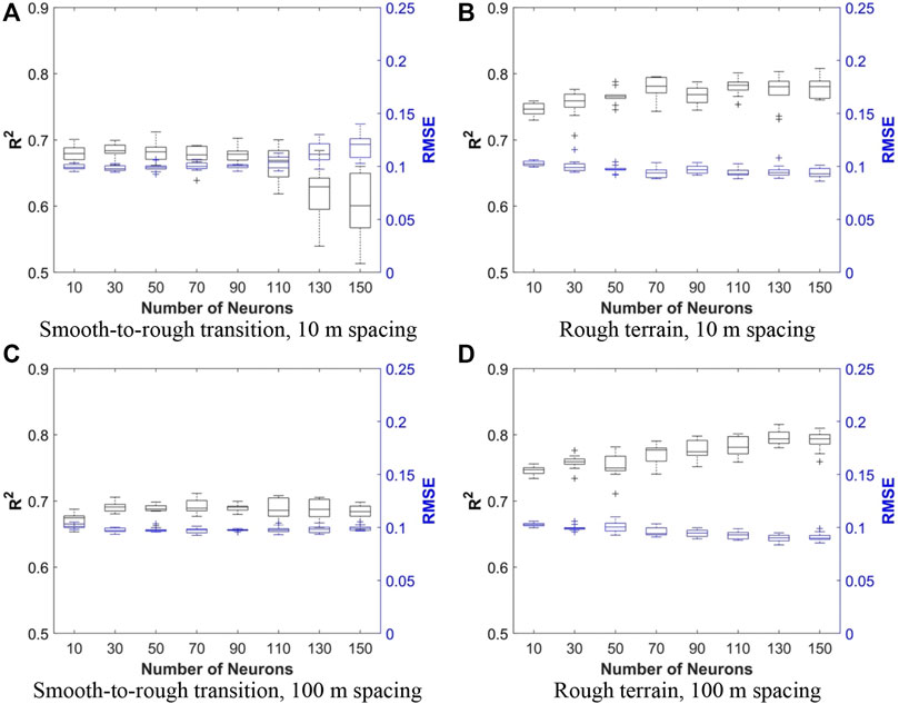
FIGURE 9. Coefficients of determination for varied neuron counts and horizontal spacing between elevation data points in the DEM for the single layer neural network. (A) Smooth-to-rough transition, 10 m spacing. (B) Rough terrain, 10 m spacing. (C) Smooth-to-rough transition, 100 m spacing. (D) Rough terrain, 100 m spacing.

FIGURE 10

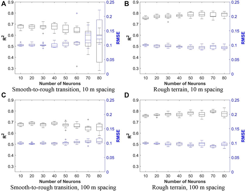
FIGURE 10. Coefficients of determination for varied neuron counts and horizontal spacing between elevation data points in the DEM for the double layer neural network. (A) Smooth-to-rough transition, 10 m spacing. (B) Rough terrain, 10 m spacing. (C) Smooth-to-rough transition, 100 m spacing. (D) Rough terrain, 100 m spacing.

In all model configurations, R² and RMSE vary little for the lower neuron counts, ranging from approximately 0.65–0.75. Larger neuron counts produce a slight improvement for the rough terrain cases but reduce the accuracy of the model for three of four smooth-to-rough transition cases. This degradation in the model is the worst for the double hidden layer case (Figure 10A). The only model that shows improvement as the number of neurons increases is the rough terrain case using 100 m horizontal fetch resolution (Figure 9D), however the marginal improvement is far outweighed by the increased computational expense. For example, training a 150 neuron model takes approximately 30 times longer than training the 10 neuron model. Similarly, the use of a fine (10 m) resolution DEM input data slowed down the training process and did not improve the performance when compared to the use of a coarse (100 m) DEM.

Figures 11, 12 present the testing, training, and validation results for two cases of the smooth-to-rough transition and rough terrain models using 30 and 150 neuron single hidden layer architectures, respectively. Data are stratified by the magnitude of the speedup value. Testing the neural network on data yields R² values of 0.67 and 0.74 (and RMSE values of 0.11 for both cases), exceeding the observed R² value of 0.5 by Chock and Cochran (2005). The neural network performance was compared to the linear regression method, using the same data for the training, and testing of the neural network. The linear model performance on the stratified data resulted in R² of 0.65 and 0.61. Notably, the neural network models exhibit less variability between runs as the speedup value increases.

FIGURE 11

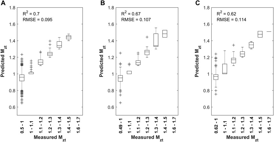
FIGURE 11. Training, testing, and validation of a single layer, 30 neuron model for the smooth-to-rough transition cases using 100 m horizonal spacing DEM data. (A) Training, (B) Testing, and (C) Validation.

FIGURE 12

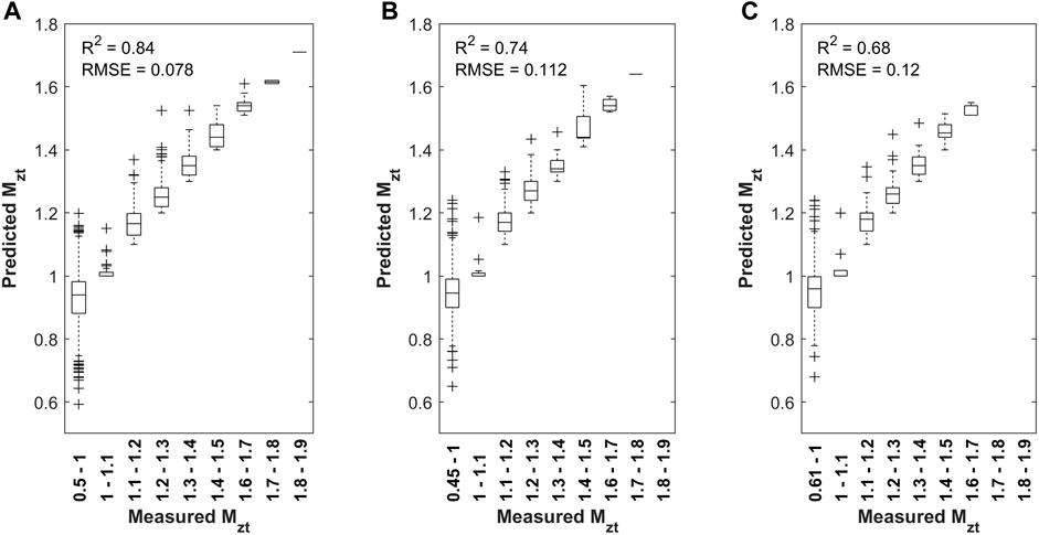
FIGURE 12. Training, testing, and validation of a single layer, 150 neuron model for the rough terrain cases using 100 m horizonal spacing DEM data. (A) Training, (B) Testing, and (C) Validation.

The encouraging results of these sensitivity tests support the use of simple configurations of neural networks for predicting topographic effect multipliers in complex terrain directly from the elevation data. To simplify this approach further, single hidden layer models were trained using data from all terrain types. This modification has the effect of reducing any benefit of stratifying the upwind terrain types but beneficially increases the size of the data available for training, testing, and validation.

Figure 13 presents the R² and RMSE box and whisker plots based on neuron count for the “all upwind terrain” case. Figure 14 presents the results from training, testing, and validation for a single model. The results yield similar R² and RMSE values as the terrain stratified model results given in Figures 9–12, indicating that stratifying the data by upwind terrain type did not produce any appreciable improvement in the modeling.

FIGURE 13

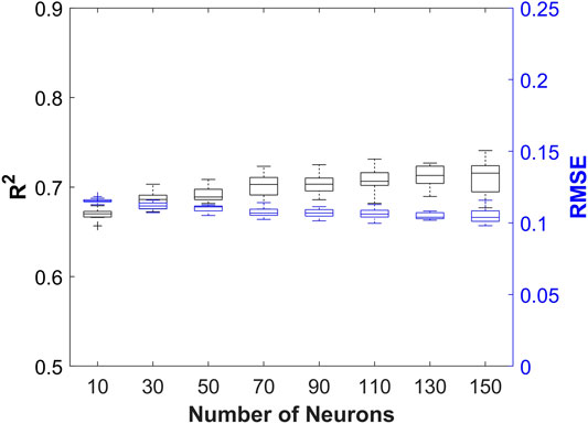
FIGURE 13. Coefficients of determination for varied neuron counts, using the single layer neural network and 100 m horizontal spacing DEM data.

FIGURE 14

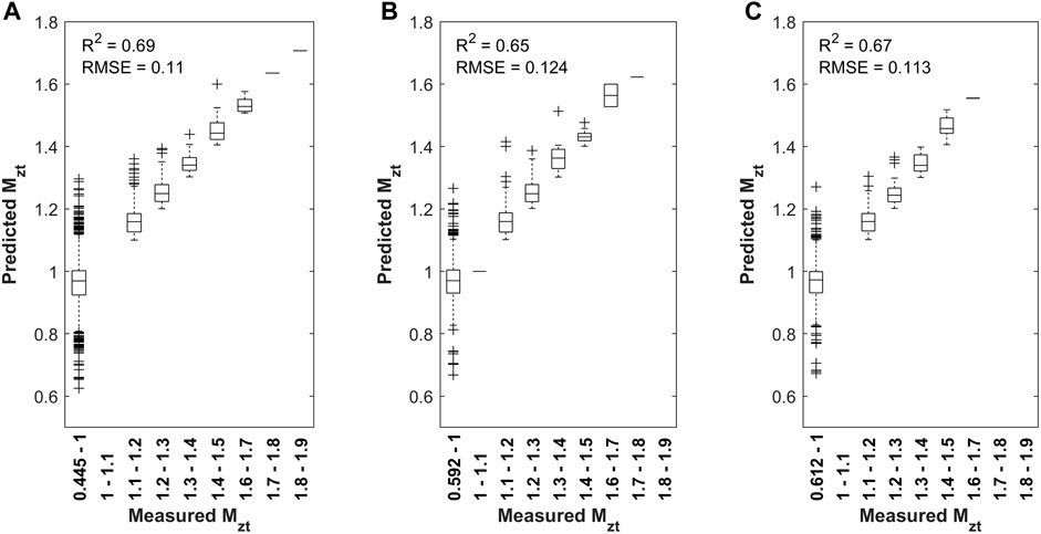
FIGURE 14. Training, testing, and validation of a single layer, 30 neuron model for all terrain cases using 100 m horizonal spacing DEM data. (A) Training (B) Testing (C) Validation.

Returning to the primary goal of producing maximum topographic effect multiplier maps, a 30-neuron model with coarse horizontal fetch resolution and no stratification of approach flow condition was trained (R² = 0.819, RMSE = 0.09) and then applied to the six study regions. To create the maps, data were extracted in a 50 m horizontal resolution grid from a gridded interpolant of the DEM data. The same DEM interpolant was then used to extract the fetch elevation data at 100 m intervals (coarse resolution) ranging from 2 km upwind to 1 km downwind for 16 wind angles. For each grid location and each wind angle, the elevation fetch data were input to the neural network to predict the gust topographic effect multiplier specific to that location and wind angle. Finally, the largest multiplier over all wind angles was determined and plotted in the Figure 15.

FIGURE 15

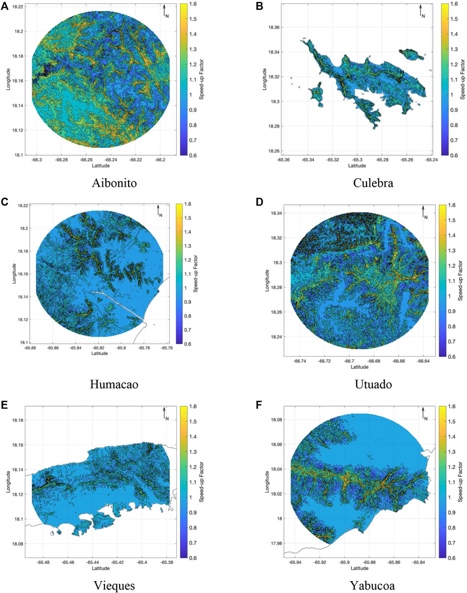
FIGURE 15. Predictions of topographic effect multipliers, enveloping for all directions. (A) Aibonito. (B) Culebra. (C) Humacao. (D) Utuado. (E) Vieques. (F) Yabucoa.

Ground truth over the study regions is not available to draw a quantitative comparison to the neural network outputs, but qualitatively it is observed that the gradation of the topographic effect multipliers matches expectations. Values are less than unity in valley regions, approach unity in flat open expanses, and reach 1.6–1.7 for the upper slopes of the mountains. The upper bound compares favorably to previous studies of topographic effect multipliers for surface gusts, e.g., Kondo et al. (2002), Glanville and Kwok (1997), and Bowen and Clucas (1992), which give values of 1.6–1.8. Further, the computational expense of producing these maps, which cover 121 km² at a 50 m resolution, is approximately 5 mins using a single compute core on a laptop. With parallelization, it should be possible to compute a map for the entire island of Puerto Rico within a day or less.

Discussion and Conclusion

The study provides initial proof-of-concept that shallow neural networks may offer an alternative and computationally inexpensive approach to produce topographic wind speedup maps such as the “special wind regions” in ASCE 7. A shallow neural network was successfully trained using digital elevation data (inputs) and surface velocity measurements taken at 25 m FS over 1:3,100 scale models of regions of Puerto Rico and its municipal islands (outputs). Training a neural network requires voluminous amounts of data, thus data collection was automated to conduct high throughput experimentation, making it possible to collect hundreds of measurements per day. Six 4 m diameter models were tested in BLWT for approximately 2 weeks, producing 5,968 records measured from 373 unique geographic locations in 16 wind directions. Feed forward neural networks were trained varying the number of hidden layers, comparing different horizontal resolutions of the DEM data (input) and by stratifying the approach flow conditions. It was ultimately found that low neuron count, single hidden layer networks are sufficient to train models to predict topographic effect multipliers, which opens the door to applying the model to similar terrain in other parts of Puerto Rico. Sensitivity studies revealed that stratifying the approach flow conditions before training and using as input a finer (10 m) resolution of the DEM data did not cause a significant improvement in the predictive performance of the neural network. Lastly, six topographic wind speedup maps provide predictions over six complex terrain regions, demonstrating the computational advantage of using this methodology.

We conclude that this approach could be extended to other terrain and land-use/land-cover (LULC) types if the BLWT dataset was expanded to other geographical regions, particularly those that possess different gross physical features, taller landforms, and landform elements atypical to the terrain evaluated in this study. Synthetic topography could also be generated from target information about elevation, slope, curvature, and rugosity, with variations in surface roughness introduced to model LULC effects. The results from these studies could be combined to create a shared global topographic wind speedup database that warehouses BLWT experimental data to validate, generalize, and cross-compare predictive modeling and ultimately reduce the need for the extremely laborious physical testing required to collect these data. Alternatively, these data could augment existing field measurement atlases such as the New European Wind Atlas (Mann et al., 2017).

Future research will be required to standardize experimental methods and data processing to achieve this vision. Our experience with this study, a thorough review of the literature, and follow up discussions with other BLWT modelers led us to identify multiple key areas that warrant further investigation. Examples of topics include:

• Revisiting the acceptable range of geometric scales. The accepted upper bounds for geometric scaling (∼1:2,500—1:6,000) appear to originate from early BLWT tests on low hills free of obstructions (e.g., trees). While the Reynolds number requirement $u_{\ast }{k}_s/\nu >70$ can be relaxed without loss of simulation accuracy (Taylor and Teunissen, 1987), it is questionable if the relaxation will hold for more complex environments (Bowen, 1983)—particularly for mountainous landforms that are (partially) covered in tree canopies. Further, the effect of geometric scale on the observed power spectra has received scarce discussion in the literature. As McAuliffe and Larose (2012) and the current (1:3,100 scale) study observed, analysis of the power spectra clearly indicate that surface (10–25 m FS) measurements sample the eddy surface layer, not the inertial sublayer.

• Defining a non-arbitrary reference wind speed in the physical simulation. The boundary layer depth varies over the model as a function of the elevation profile, and mountain heights can exceed the boundary layer depth by a factor of five or more. Adopting the surface wind speed upwind of the model also introduces variability between tests of different models. Internal boundary layers form between the end of the development section and the model (causing wind speed recovery), and the presence of the land mass retards the wind speed well before it reaches the landform.

• Modeling topographic features that extend to or beyond the perimeter of the model, e.g., a region within a mountain chain. Most of the study subjects in the experimental research literature are isolated landforms that terminate upwind into a flat expanse. While we would assert that the taper-fetch-test partitioning (Figure 7) is a rational approach to prevent an abrupt transition, additional work is required to move this heuristic approach into an analytical framework. This guidance should also address the modelling of the upper part of a tall landform.

• Modeling (heterogenous) surface roughness and, as a practical matter, doing so without prohibitively increasing fabrication time/cost. Today topographic models are usually fabricated through subtractive manufacturing, e.g., the 3-axis CNC used in this study. This tried-and-true approach should either be replaced with large-scale additive manufacturing (e.g., 3D printing) or a 4- or 5-axis CNC to simultaneously impart the desired shape and surface roughness.

Data Availability Statement

Data are available through the National Science Foundation Engineering Research Infrastructure DesignSafe site at https://doi.org/10.17603/ds2-2gab-dw61.

Author Contributions

RC led the model fabrication, wind tunnel simulations, and data collection efforts. ARS performed the pilot study to evaluate the efficacy of the machine learning algorithm. JXS-H improved on this algorithm and co-authored the paper, under the supervision of LDA-B and FM. BP scaled up the algorithm for the wind map production and provided input to the manuscript. FM provided overall oversight of the project and co-wrote the manuscript.

Funding

Support for this research was provided by the NSF EAGER award (No. CMMI-1841979) with additional support for experimentation through the NSF Natural Hazards Engineering Research Infrastructure (NHERI) program (CMMI-1520843). We would also like to acknowledge the NSF Research Experiences for Undergraduates (REU) program for supporting co-author ARS for performing the initial study that led to the work documented herein. Data collection was performed with the support of the Strategic Alliance for Risk Reduction II (STARR II) program, which was funded by the Federal Emergency Management Agency.

Conflict of Interest

The authors declare that the research was conducted in the absence of any commercial or financial relationships that could be construed as a potential conflict of interest.

Publisher’s Note

All claims expressed in this article are solely those of the authors and do not necessarily represent those of their affiliated organizations, or those of the publisher, the editors and the reviewers. Any product that may be evaluated in this article, or claim that may be made by its manufacturer, is not guaranteed or endorsed by the publisher.

Acknowledgments

The authors wish to recognize the Powell Family Structures and Materials Laboratory staff, with special thanks to Eric Agostinelli, Kevin Stultz, and Shelby Brothers for their contribution in wind tunnel testing. Special thanks are extended to Fernando Carmona-Esteva for his feedback and assistance during the neural network development. Any opinions, findings, and conclusion or recommendations expressed in this paper are those of the authors and do not necessarily reflect the views of the sponsors, partners, and contributors.

Supplementary Material

The Supplementary Material for this article can be found online at: https://www.frontiersin.org/articles/10.3389/fbuil.2022.762054/full#supplementary-material

Footnotes

¹These data will be made publicly available prior to publication of the manuscript (remove this footnote later and update URL in text with more specific link via DOI). Requests for the data can be made to the corresponding author prior to its release.

References

Abdi, D. S., and Bitsuamlak, G. T. (2014). Wind Flow Simulations on Idealized and Real Complex Terrain Using Various Turbulence Models. Adv. Eng. Softw. 75, 30–41. doi:10.1016/j.advengsoft.2014.05.002

CrossRef Full Text | Google Scholar

ANSI (American National Standards Institute) (2007). Laboratory Methods of Testing Fans for Certified Aerodynamic Performance Rating ANSI/AMCA 210-07, ANSI/ASHRAE 51-07. Washington, DC: ANSI.

Google Scholar

Badger, J., Frank, H., Hahmann, A. N., and Giebel, G. (2014). Wind-Climate Estimation Based on Mesoscale and Microscale Modeling: Statistical-Dynamical Downscaling for Wind Energy Applications. J. Appl. Meteorology Climatology 53 (8), 1901–1919. doi:10.1175/JAMC-D-13-0147.1

CrossRef Full Text | Google Scholar

Baker, C. J., Wood, C. J., and Gawthorpe, R. G. (1985). Strong Winds in Complicated Hilly Terrain — Field Measurements and Wind-Tunnel Study. J. Wind Eng. Ind. Aerodyn. 18 (1), 1–26. doi:10.1016/0167-6105(85)90072-8

CrossRef Full Text | Google Scholar

Balderrama, J. A., Masters, F. J., and Gurley, K. R. (2012). Peak Factor Estimation in Hurricane Surface Winds. J. Wind Eng. Ind. Aerodynamics 102, 1–13. doi:10.1016/j.jweia.2011.12.003

CrossRef Full Text | Google Scholar

Barthelmie, R. J., Hansen, K., Frandsen, S. T., Rathmann, O., Schepers, J. G., Schlez, W., et al. (2009). Modelling and Measuring Flow and Wind Turbine Wakes in Large Wind Farms Offshore. Wind Energy 12 (5), 431–444. doi:10.1002/we.348

CrossRef Full Text | Google Scholar

Bass, D., O’Connor, B., and Perotin, M. (2018). “A Summary of Findings from FEMA’s Mitigation Assessment Team Evaluation of Texas Coastal Communities Impacted by Hurricane Harvey,” in Forensic Engineering 2018: Forging Forensic Frontiers (Reston, VA: American Society of Civil Engineers), 833–845.

Google Scholar

Bendat, J. S., Piersol, A. G., and Piersol, A. G. (2000). Random Data: Wiley Series in Probability and Statistics: Texts and References Section New York: Wiley.

Google Scholar

Bitsuamlak, G. T., Bédard, C., and Stathopoulos, T. (2007). Modeling the Effect of Topography on Wind Flow Using a Combined Numerical-Neural Network Approach. J. Comput. Civ. Eng. 21 (6), 384–392. doi:10.1061/(asce)0887-3801(2007)21:6(384)

CrossRef Full Text | Google Scholar

Bitsuamlak, G. T., Stathopoulos, T., and Bédard, C. (2002). “Neural Network Predictions of Wind Flow over Complex Terrain,” in 4th Structural Specialty Conference. of the Canadian Society for Civil Engineering, Montréal, Québec, Canada, 5–8 June, 2002.

Google Scholar

Bowen, A. J. (1983). The Prediction of Mean Wind Speed Above Simple 2D Hill Shapes. J. Wind Eng. Ind. Aerodyn. 15 (1–3), 259–270. doi:10.1016/0167-6105(83)90196-4

CrossRef Full Text | Google Scholar

Bowen, A. J., and Clucas, H. (1992). The Measurement and Interpretation of Peak-Gust Wind-Speeds over an Isolated Hill. J. Wind Eng. Ind. Aerodynamics 41 (1-3), 381–392. doi:10.1016/0167-6105(92)90436-e

CrossRef Full Text | Google Scholar

Brahimi, T. (2019). Using Artificial Intelligence to Predict Wind Speed for Energy Application in Saudi Arabia. Energies 12 (24), 4669. doi:10.3390/en12244669

CrossRef Full Text | Google Scholar

Burlando, M., and Meissner, C. (2017). Evaluation of Two ANN Approaches for the Wind Power Forecast in a Mountainous Site. Int. J. Renew. Energ. Res. (Ijrer) 7 (4), 1629–1638. doi:10.20508/ijrer.v7i4.6186.g7203

CrossRef Full Text | Google Scholar

Catarelli, R. A., Fernández-Cabán, P. L., Masters, F. J., Bridge, J. A., Gurley, K. R., and Matyas, C. J. (2020). Automated Terrain Generation for Precise Atmospheric Boundary Layer Simulation in the Wind Tunnel. J. Wind Eng. Ind. Aerodynamics 207, 104276. doi:10.1016/j.jweia.2020.104276

CrossRef Full Text | Google Scholar

Chen, J., Zeng, G.-Q., Zhou, W., Du, W., and Lu, K.-D. (2018). Wind Speed Forecasting Using Non-Linear-Learning Ensemble of Deep Learning Time Series Prediction and Extremal Optimization. Energ. Convers. Manage. 165, 681–695. doi:10.1016/j.enconman.2018.03.098

CrossRef Full Text | Google Scholar

Chen, J., Haynes, B. S., and Fletcher, D. F. (2000). Cobra Probe Measurements of Mean Velocities, Reynolds Stresses and Higher-Order Velocity Correlations in Pipe Flow. Exp. Therm. Fluid Sci. 21 (4), 206–217. doi:10.1016/s0894-1777(00)00004-2

CrossRef Full Text | Google Scholar

Chock, G. Y. K., and Cochran, L. (2005). Modeling of Topographic Wind Speed Effects in Hawaii. J. Wind Eng. Ind. Aerodynamics 93 (8), 623–638. doi:10.1016/j.jweia.2005.06.002

CrossRef Full Text | Google Scholar

Deaves, D. M. (1980). Computations of Wind Flow over Two-Dimensional Hills and Embankments. J. Wind Eng. Ind. Aerodynamics 6 (1-2), 89–111. doi:10.1016/0167-6105(80)90024-0

CrossRef Full Text | Google Scholar

Donadio, L., Fang, J., and Porté-Agel, F. (2021). Numerical Weather Prediction and Artificial Neural Network Coupling for Wind Energy Forecast. Energies 14 (2), 338. doi:10.3390/en14020338

CrossRef Full Text | Google Scholar

Finnigan, J., Ayotte, K., Harman, I., Katul, G., Oldroyd, H., Patton, E., et al. (2020). Boundary-Layer Flow Over Complex Topography. Boundary-Layer Meteorology 177 (2), 247–313. doi:10.1007/s10546-020-00564-3

CrossRef Full Text | Google Scholar

Glanville, M. J., and Kwok, K. C. S. (1997). Measurements of Topographic Multipliers and Flow Separation from a Steep Escarpment. Part II. Model-Scale Measurements. J. Wind Eng. Ind. Aerodynamics 69-71, 893–902. doi:10.1016/s0167-6105(97)00215-8

CrossRef Full Text | Google Scholar

Hagan, M. T., and Menhaj, M. B. (1994). Training Feedforward Networks with the Marquardt Algorithm. IEEE Trans. Neural Netw. 5 (6), 989–993. doi:10.1109/72.329697

PubMed Abstract | CrossRef Full Text | Google Scholar

Haupt, S. E., Kosovic, B., Shaw, W., Berg, L. K., Churchfield, M., Cline, J., et al. (2019). On Bridging A Modeling Scale Gap: Mesoscale to Microscale Coupling for Wind Energy. Bull. Am. Meteorol. Soc. 100 (12), 2533–2550. doi:10.1175/bams-d-18-0033.1

CrossRef Full Text | Google Scholar

Hornik, K., Stinchcombe, M., and White, H. (1989). Multilayer Feedforward Networks Are Universal Approximators. Neural Networks 2 (5), 359–366. doi:10.1016/0893-6080(89)90020-8

CrossRef Full Text | Google Scholar

Huang, W. F., and Xu, Y. L. (2013). Prediction of Typhoon Design Wind Speed and Profile over Complex Terrain. Struct. Eng. Mech. 45 (1), 1–18. doi:10.12989/sem.2013.45.1.001

CrossRef Full Text | Google Scholar

Jackson, P. S., and Hunt, J. C. R. (1975). Turbulent Wind Flow over a Low Hill. Q.J R. Met. Soc. 101 (430), 929–955. doi:10.1002/qj.49710143015

CrossRef Full Text | Google Scholar

Jenness, J. (2013). DEM Surface Tools for ArcGIS. Flagstaff, AZ, USA: Jenness Enterprises. Available at: http://www.jennessent.com/arcgis/surface_area.htm.

Google Scholar

Kikuchi, Y., and Ishihara, T. (2012). “A Study of Topographic Multiplier Considering the Effect of Complex Terrains and Tropical Cyclones. J. Wind Eng. Indus. Aero. 104–106, 558–564. doi:10.1016/j.jweia.2012.04.008

PubMed Abstract | CrossRef Full Text | Google Scholar

Kishore, N., Marqués, D., Mahmud, A., Kiang, M. V., Rodriguez, I., Fuller, A., et al. (2018). Mortality in Puerto Rico After Hurricane Maria. N. Engl. J. Med. 379 (2), 162–170. doi:10.1056/nejmsa1803972

PubMed Abstract | CrossRef Full Text | Google Scholar

Križan, J., Gašparac, G., Kozmar, H., Antonić, O., and Grisogono, B. (2015). Designing Laboratory Wind Simulations Using Artificial Neural Networks. Theor. Appl. Climatology 120 (3), 723–736. doi:10.1007/s00704-014-1201-4

CrossRef Full Text | Google Scholar

Kondo, K., Tsuchiya, M., and Sanada, S. (2002). Evaluation of Effect of Micro-Topography on Design Wind Velocity. J. Wind Eng. Ind. Aerodyn. 90 (12–15), 1707–1718. doi:10.1016/s0167-6105(02)00281-7

CrossRef Full Text | Google Scholar

Kwasinski, A., Andrade, F., Castro-Sitiriche, M. J., and O’Neill-Carrillo, E. (2019). Hurricane Maria Effects on Puerto Rico Electric Power Infrastructure. IEEE Power Energy Tech. Sys. J. 6 (1), 85–94. doi:10.1109/jpets.2019.2900293

CrossRef Full Text | Google Scholar

Lange, J. (2016). Flow Over Complex Terrain. The Secrets of Bolund. DTU Wind Energy. DTU Wind Energy. PhD Thesis.

Google Scholar

Liu, H. (2010). “On the Levenberg-Marquardt Training Method for Feed-Forward Neural Networks,” in 2010 Sixth International Conference on Natural Computation, Yangchai, China, 10–12 August 2010. IEEE, 1, 456–460. doi:10.1109/icnc.2010.5583151

CrossRef Full Text | Google Scholar

Liu, H., Mi, X., and Li, Y. (2018). Smart Deep Learning Based Wind Speed Prediction Model Using Wavelet Packet Decomposition, Convolutional Neural Network and Convolutional Long Short Term Memory Network. Energy Convers. Manag. 166, 120–131. doi:10.1016/j.enconman.2018.04.021

CrossRef Full Text | Google Scholar

Lubitz, W. D., and White, B. R. (2007). Wind-Tunnel and Field Investigation of the Effect of Local Wind Direction on Speed-Up Over Hills. J. Wind Eng. Ind. Aerodyn. 95 (8), 639–661. doi:10.1016/j.jweia.2006.09.001

CrossRef Full Text | Google Scholar

Mann, J., Angelou, N., Arnqvist, J., Callies, D., Cantero, E., Arroyo, R. C., et al. (2017). Complex Terrain Experiments in the New European Wind Atlas. Phil. Trans. R. Soc. A. 375, 20160101. doi:10.1098/rsta.2016.0101

PubMed Abstract | CrossRef Full Text | Google Scholar

Masters, F., and Catarelli, R. (2022). “Surface Wind Speed Measurements Over Reduced-Scale Topographic Models of Select Regions in Puerto Rico in a Large BLWT,” in Modeling of Wind Speed Up for Microzoning of Design Wind Speeds in Puerto Rico (DesignSafe-CI). Available at: https://doi.org/10.17603/ds2-2gab-dw61.

Google Scholar

Mayo, M., Wakes, S., and Anderson, C. (2018). “Neural Networks for Predicting the Output of Wind Flow Simulations Over Complex Topographies,” in 2018 IEEE International Conference on Big Knowledge (ICBK), Singapore, 17–18 Nov 2018. IEEE, 184.

CrossRef Full Text | Google Scholar

McAuliffe, B. R., and Larose, G. L. (2012). Reynolds-Number and Surface-Modeling Sensitivities for Experimental Simulation of Flow Over Complex Topography. J. Wind Eng. Ind. Aerodynamics 104-106, 603–613. doi:10.1016/j.jweia.2012.03.016

CrossRef Full Text | Google Scholar

Ngo, T. T., and Letchford, C. W. (2009). Experimental Study of Topographic Effects on Gust Wind Speed. J. Wind Eng. Ind. Aerodynamics 97 (9-10), 426–438. doi:10.1016/j.jweia.2009.06.013

CrossRef Full Text | Google Scholar

Olson, J. B., Kenyon, J. S., Djalalova, I., Bianco, L., Turner, D. D., Pichugina, Y., et al. (2019). Improving Wind Energy Forecasting Through Numerical Weather Prediction Model Development. Bull. Am. Meteorol. Soc. 100 (11), 2201–2220. doi:10.1175/BAMS-D-18-0040.1

CrossRef Full Text | Google Scholar

Pasch, R. J., Penny, A. B., and Berg, R. (2019). National Hurricane Center Tropical Cyclone Report: Hurricane Maria (AL152017). Available at: www.nhc.noaa.gov/data/tcr/AL152017_Maria.pdf. (Accessed February 14, 2019).

Google Scholar

Prevatt, D. O., Roueche, D. B., Aponte-Bermudez, L. D., Kijewski-Correa, T., Li, Y., Chardon, P., et al. (2018). “Performance of Structures Under Successive Hurricanes: Observations from Puerto Rico and the US Virgin Islands After Hurricane Maria,” in Forensic Engineering 2018: Forging Forensic Frontiers (Reston, VA: American Society of Civil Engineers), 1049–1059. doi:10.1061/9780784482018.101

CrossRef Full Text | Google Scholar

Quill, R., Sharples, J. J., and Sidhu, L. A. (2020). A Statistical Approach to Understanding Canopy Winds Over Complex Terrain. Environ. Model. Assess. 25 (2), 231–250. doi:10.1007/s10666-019-09674-w

CrossRef Full Text | Google Scholar

Rasouli, A., Hangan, H., and Siddiqui, K. (2009). PIV Measurements for a Complex Topographic Terrain. J. Wind Eng. Ind. Aerodynamics 97 (5-6), 242–254. doi:10.1016/j.jweia.2009.06.010

CrossRef Full Text | Google Scholar

Robert, S., Foresti, L., and Kanevski, M. (2013). Spatial Prediction of Monthly Wind Speeds in Complex Terrain With Adaptive General Regression Neural Networks. Int. J. Climatol. 33 (7), 1793–1804. doi:10.1002/joc.3550

CrossRef Full Text | Google Scholar

Salmon, J. R., Bowen, A. J., Hoff, A. M., Johnson, R., Mickle, R. E., Taylor, P. A., et al. (1998). The Askervein Hill Project: Mean Wind Variations at Fixed Heights Above Ground. Boundary-Layer Eteorology 43, 247–271.

Google Scholar

Santoni, C., García‐Cartagena, E. J., Ciri, U., Zhan, L., Valerio Iungo, G., and Leonardi, S. (2020). One‐Way Mesoscale‐Microscale Coupling for Simulating a Wind Farm in North Texas: Assessment Against SCADA and LiDAR Data. Wind Energy 23 (3), 691–710. doi:10.1002/we.2452

CrossRef Full Text | Google Scholar

Sutton, O. G. (1949). The Application to Micrometeorology of the Theory of Turbulent Flow Over Rough Surfaces. Q.J R. Met. Soc. 75 (326), 335–350. doi:10.1002/qj.49707532602

CrossRef Full Text | Google Scholar

Taylor, P. A., and Teunissen, H. W. (1987). The Askervein Hill Project: Overview and Background Data. Boundary-Layer Meteorology 39 (1-2), 15–39. doi:10.1007/bf00121863

CrossRef Full Text | Google Scholar

von Kármán, T. (1948). Progress in the Statistical Theory of Turbulence. Proc. Natl. Acad. Sci. 34 (11), 530–539. doi:10.1073/pnas.34.11.530

CrossRef Full Text | Google Scholar

Wilczak, J., Finley, C., Freedman, J., Cline, J., Bianco, L., Olson, J., et al. (2015). The Wind Forecast Improvement Project (WFIP): A Public-Private Partnership Addressing Wind Energy Forecast Needs. Bull. Am. Meteorol. Soc. 96 (10), 1699–1718. doi:10.1175/bams-d-14-00107.1

CrossRef Full Text | Google Scholar

Yu, C., Li, Y., Xiang, H., and Zhang, M. (2018). Data Mining-Assisted Short-Term Wind Speed Forecasting by Wavelet Packet Decomposition and Elman Neural Network. J. Wind Eng. Ind. Aerodynamics 175, 136–143. doi:10.1016/j.jweia.2018.01.020

CrossRef Full Text | Google Scholar