Partitioning QUBO with two-way one-hot conditions on traveling salesman problems for city distributions with multiple clusters

1 Introduction

Recently, Ising machines based on simulated and quantum annealing, etc., have been actively used to solve combinatorial optimization problems (COPs) at high speed and are beginning to be applied to realistic business problems (Neukart et al., 2017; Nishimura et al., 2019; Ohzeki et al., 2019; Kanamaru et al., 2021; NEC Corporation, 2022a, 2023; Yarkoni et al., 2022; Mori and Furukawa, 2023) as well as academic problems (Bando et al., 2020; Abel et al., 2021; Mniszewski et al., 2021; Mukai and Kudo, 2021; Gaidai et al., 2022). There have also been many studies on typical problems that have a wide range of applications (Ushijima-Mwesigwa et al., 2017; Quintero et al., 2022; Salehi et al., 2022; Suen et al., 2022), those on performance benchmarking to demonstrate the usefulness of Ising machines (King et al., 2015, 2019; Lubinski et al., 2023) and those on improving the performance of the Ising machine relating to pre-processing (Oku et al., 2020; Yachi et al., 2023), embedding (Okada et al., 2019b; Bernal et al., 2020), and post-processing (Pudenz et al., 2015; Borle and McCarter, 2019).

The quantum annealing machines currently in practical use [e.g., D-Wave Advantage (D-Wave Quantum Inc., 2023b)] alone can solve COPs with up to ~120 bits in case of the complete graph [equivalent to about 10 cities in the traveling salesman problem (TSP) (Warren, 2020; Jain, 2021)]. However, real-world problems are often large. Ising machines based on simulated annealing are helpful for such applications.

In addition, quantum-classical hybrid algorithms that combine quantum annealing with conventional computing techniques are practical. One such example is D-Wave Hybrid (D-Wave Quantum Inc., 2023a; Raymond et al., 2023). In the hybrid algorithm with using quantum annealing, a problem is divided and converted to the size that a quantum annealing machine can compute. Therefore, it is essential to have an algorithm that solves COPs with a good partitioning technique.

The earliest hybrid algorithm, qbsolv (Booth et al., 2017; D-Wave Quantum Inc., 2021), combines tabu search and quantum annealing and repeatedly solves the Ising or QUBO model to find a solution. This allows us to solve COPs of a scale that cannot be solved by quantum annealing alone. In the following, the hybrid algorithms using Ising machines other than quantum annealing are also called hybrid algorithms.

There are also hybrid algorithms that have algorithms for partitioning the problem to a scale that can be solved by an Ising machine (Atobe et al., 2021; Irie et al., 2021), and hybrid algorithms that use the computation on an Ising machine as a subroutine (Chancellor, 2017, 2023; Kitai et al., 2020; Ohzeki, 2020; Izawa et al., 2022). Various hybrid algorithms have been proposed for particular problems, and their effectiveness has been verified (Bian et al., 2016; Abbott et al., 2019; Feld et al., 2019; Okada et al., 2019a; Shaydulin et al., 2019; Ushijima-Mwesigwa et al., 2021; Liu et al., 2022).

On the other hand, even when solving with simulated annealing, obtaining a near-optimal solution in a shorter time is often easier if the number of variables is small than in the case of a large problem. Because of this, even when solving COPs with simulated annealing, it is considered important to partition the problem and reduce the number of variables according to the context of the problem to be solved.

However, to perform problem partitioning, users must be familiar with simulated and quantum annealing. Users who need to become more familiar with Ising machines will likely let the Ising machine solve the problem as it is without dividing the problem.

The large number of variables also makes the problem more challenging to solve in terms of satisfying constraint conditions. Constraints are conditions that must be satisfied by the solution obtained by the Ising machine. For example, in the QUBO, a constraint called the one-hot condition often appears, where only one of the variables in a set has the value one and the others have the value 0. COPs with constraints are more complex than those without constraints because the obtained solution cannot be interpreted as a meaningful solution unless all the given constraints are satisfied. Methods of partitioning for specific problems with one-hot conditions have also been proposed for the quadratic assignment problem (Nishimura et al., 2019) and for the integer programming problem (Okada et al., 2019a).

In this study, we consider how to partition the TSP, an example of a problem with constraints, from a QUBO matrix, a commonly used input format for Ising machines. In particular, we aim to automatically divide the problem so that even users unfamiliar with the Ising machine can benefit from the problem division. In Section 2, we describe the two-way one-hot constraints and the formulation of the traveling salesman problem. Section 3 deals with concrete methods for splitting the traveling salesman problem. We solve the traveling salesman problem of clustered cities by our proposed methods in Section 4 and discuss the limitations of the proposed method, a comparison with 2-opt and how to apply them to other types of problems in Section 5. Finally, Section 6 summarizes the contents of this study.

2 Two-way one-hot constraints and traveling salesman problems

2.1 Two-way one-hot constraints

To solve COPs by Ising machines, one inputs a Hamiltonian formulated in an Ising model or a quadratic unconstrained binary optimization (QUBO). An Ising model is represented by a quadratic function in spin variables (σ_i ∈ {+1, −1}), and a QUBO is expressed as a quadratic function in binary variables (x_i ∈ {0, 1}). An input Hamiltonian H contains information on the constraints, which must be satisfied in the solution, and that on the objective function, which reflects the state of the solution to be aimed for,

$\begin{array}{ll}H=C_C{H}_C+C_O{H}_O.& (1)\end{array}$

In Equation (1) H_C and H_O represent Hamiltonians for the constraints and the objective function, respectively, and C_C and C_O stand for coefficient parameters of the constraints and the objective functions.

The one-hot constraint often appears when formulating COPs in QUBO. It is a constraint where only one variable in a set of variables has a value of one, and the rest have a value of 0, which is shown as Equation (2) for N variables x_i (0 ≤ i ≤ N − 1).

$\begin{array}{ll}{\displaystyle \sum _{i=0}^{N-1}}{x}_i=1& (2)\end{array}$

It is used in situations where one of several items must be chosen. For example, in a clustering problem, it is used to ensure that each element is included in one of the clusters. It can also be used to select one numerical value from several values (“one-hot encoding").

Some COPs have the two-way one-hot constraint, which has one-hot conditions for each row and each column in a two-dimensional array variable with the same number of rows and columns. It may be easier to understand if variables x_ij are written in a table. For example, if the first index i corresponds to a row and the second j to a column, it can be represented as shown in Figure 1. The example is the case of a TSP for four cities, the variables of which are shown by the table of four rows and four columns.

Figure 1

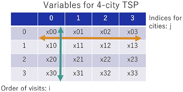
Figure 1. Four-city TSP variable have a two-way one-hot constraint. When the variables are represented in a table, there are vertical and horizontal one-hot conditions.

For binary variables x_ij (0 ≤ i, j ≤ N − 1), a two-way one-hot constraint is represented as the following set of equations:

$\begin{array}{ll}{\displaystyle \sum _{j=0}^{N-1}}{x}_{ij}=1\text{ for }0\le i\le N-1,& (3)\end{array}$

$\begin{array}{ll}{\displaystyle \sum _{i=0}^{N-1}}{x}_{ij}=1\text{ for }0\le j\le N-1.& (4)\end{array}$

These constraints are expressed as the Hamiltonian of the QUBO formulation as follows:

$\begin{array}{ll}{\displaystyle \sum _{i=0}^{N-1}}{\left({\displaystyle \sum _{j=0}^{N-1}}{x}_{ij}-1\right)}^2,& (5)\end{array}$

$\begin{array}{ll}{\displaystyle \sum _{j=0}^{N-1}}{\left({\displaystyle \sum _{i=0}^{N-1}}{x}_{ij}-1\right)}^2.& (6)\end{array}$

If one now arranges the variable x_ij in a two-dimensional array as in Figure 1, where i corresponds to the rows and j to the columns, Equations (3, 5) are the one-hot condition for the horizontal direction. Represented in terms of an array of a QUBO matrix, it corresponds to the components arranged in a triangular form along the diagonal components of the QUBO matrix as shown in Figure 2, where QUBO matrices are upper triangular matrices.

Figure 2

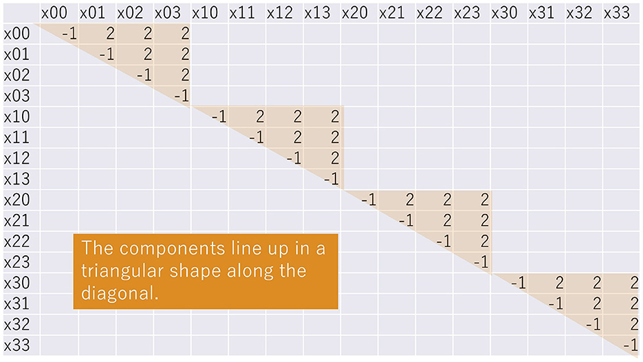
Figure 2. QUBO matrix components representing the one-hot condition for the horizontal direction corresponding to Equation (3).

On the other hand, Equations (4, 6) are the one-hot condition for the vertical direction in Figure 1. The QUBO matrix represented by the upper triangular matrix is shown in Figure 3 if one arranges x_ij in a two-dimensional array as in Figure 2. The components are aligned in the direction parallel to the diagonal components of the QUBO matrix.

Figure 3

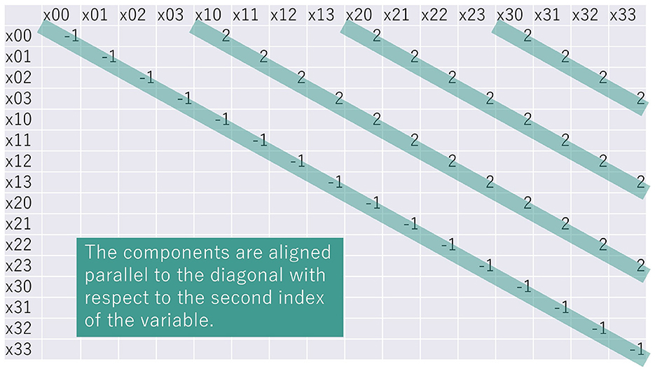
Figure 3. QUBO matrix components representing the one-hot condition for the vertical direction corresponding to Equation (4).

Problems that determine order or assignment, such as the TSPs and the quadratic assignment problems (QAPs), are formulated using the two-way one-hot condition.

2.2 Traveling salesman problems

A TSP aims to minimize travel distance while meeting these two-way one-hot constraints. To minimize the total travel distance to visit cities, Equation (7) is added to the Hamiltonian as the objective function, where d_jk denotes the distance between city j and city k.

$\begin{array}{ll}{\displaystyle \sum _{i=0}^{N-2}}{\displaystyle \sum _{j\ne k}}{d}_{jk}{x}_{ij}{x}_{i+1,k}+{\displaystyle \sum _{j\ne k}}{d}_{jk}{x}_{N-1,j}{x}_{0,k}& (7)\end{array}$

The QUBO matrix for the objective function is shown in the lower table in Figure 4. In the QUBO matrix, the matrix of distances between cities (the upper table in Figure 4) appears with the first subscript of the variable shifted by one. In addition, since the TSP considers a circuitous route, a matrix of distances also appears in the upper right part of the QUBO matrix to add the distance of the route from the last city visited to the first city visited.

Figure 4

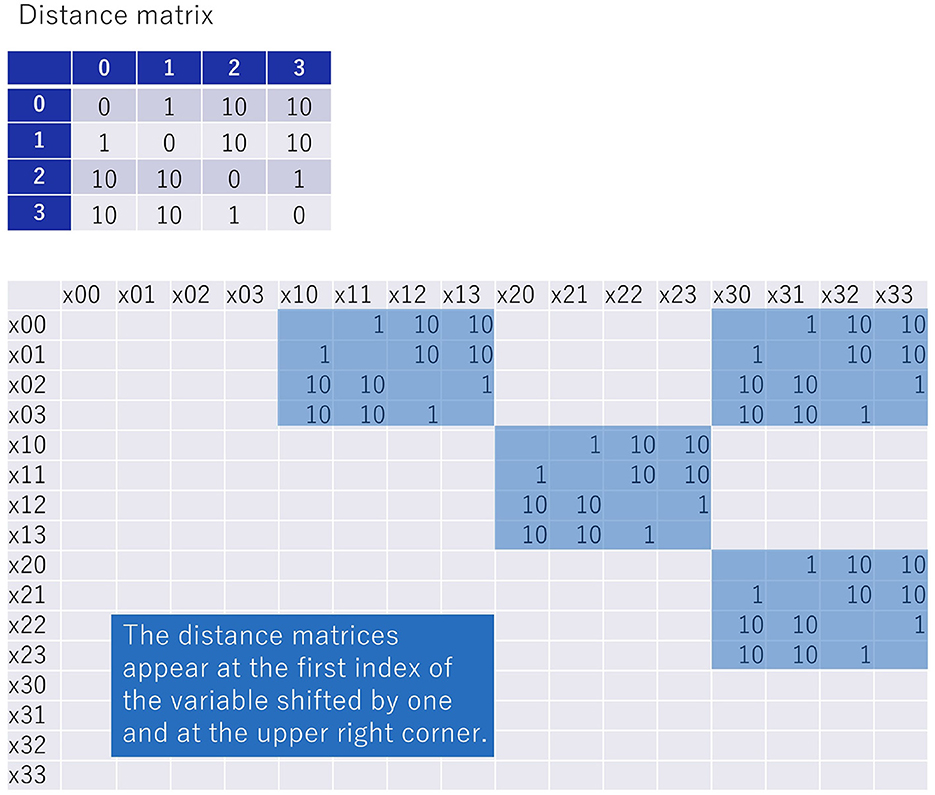
Figure 4. QUBO matrix corresponding to the objective function of the TSP contains a series of matrices representing distances between cities.

The TSP Hamiltonian and QUBO matrices are a combination of the one-hot constraint part (Equations 5, 6) and the objective function part (Equation 7). Since we aim to minimize the objective function under the constraints, the QUBO matrix should be adjusted so that the constraint condition part is more significant than the objective function part. Therefore, coefficients are applied to the Hamiltonian or QUBO matrix of the constraint and objective function parts as Equation (1).

3 Method

3.1 Idea of division

In this study, we aim to allow users unfamiliar with Ising machines to benefit from partitioning even when inputting the QUBO matrix as is. For this purpose, we consider partitioning the input QUBO matrix without explicitly stating that the input is the Hamiltonian of the TSP or inputting information unique to the TSP, such as the coordinates of cities. In addition, unlike problem partitioning that clusters cities from their coordinates, the method proposed in this article uses only information on the components of the QUBO matrix. In this respect, this study differs from studies about the clustering (Bauckhage et al., 2018; Kumagai et al., 2021; Matsumoto et al., 2022).

The QUBO matrix of TSP contains submatrices of distance d_jk between cities. We call these submatrices of distance values the “distance matrices," an example of which is “distance matrix" of Figure 4. Figure 5 illustrates the idea of clustering cities using the distance matrix. This figure deals with a distance matrix for six cities, where cities 0, 1, 2 and, 3, 4, 5 are distributed in clusters. The distance matrix shows that the distance between one of the cities 0, 1, 2 and one of the cities 3, 4, 5 (circled in blue) is larger than the distance between the cities 0, 1, 2 (circled in orange) and the distance between the cities 3, 4, 5 (circled in green). Since TSP aims to keep distances as small as possible, we can expect that pathways corresponding to components within the orange and green regions would be more likely to appear than pathways corresponding to the blue region. For this reason, we will adopt the procedure of ignoring the distance in the blue part, solving the TSP for the orange and green parts independently, and considering the blue part later.

Figure 5

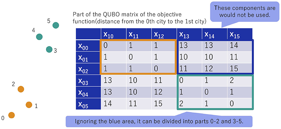
Figure 5. Idea of clustering cities using the distance matrix, which is part of objective function of the QUBO matrix.

When dividing a TSP, it is useful to pay attention to the objective function part of the QUBO matrix and the distance matrix. The constraint conditions of TSP are only two-way one-hot conditions, and the shapes of their QUBO matrices are predictable, as shown in Figures 2, 3. Therefore, it may be possible to extract the part of the objective function from the QUBO matrix by determining the coefficients of the constraint condition to remove the diagonal component since there is no diagonal component such as (x00, x00) in the objective function of the QUBO matrix. Removing the constraint conditions is also possible by using an Ising machine or middleware that allows the explicit input of constraints and Hamiltonians that represent the constraint conditions. “Flip option" in Ising machine “Vector Annealing" (NEC Corporation, 2022b) and “Constraint" in middleware “PyQUBO" (Zaman et al., 2021; Recruit Communications Co., Ltd., 2022) are examples of such functions.

After extracting the objective function part of the QUBO matrix, one obtains the distance matrix. The QUBO matrix of the objective function part contains the matrices of distance, as shown in Figure 4. Since each matrix is equal, any one of them can be used as the distance matrix.

By the way, when cities included in the same cluster correspond to adjacent indices as in Figure 5, clustering of cities is possible as cities corresponding to orange and green areas within the distace matrix. If cities not in the same cluster correspond to adjacent indices, it appears that clustering is not possible using only the information from the QUBO matrix, but it may turn out that clustering of cities is possible by redefining the indices as in Figure 6. In the example shown in Figure 6, one needs to repeat sorting by distance from one city to the other cities in ascending order starting from the 0'th city. In this way, redefining the indices so that the indices of cities that are likely to be in the same cluster are adjacent to each other, we get 0' → 0, 1' → 3, 2' → 4, 3' → 2, 4' → 5, 5' → 1 and the same distance matrix of Figure 5.

Figure 6

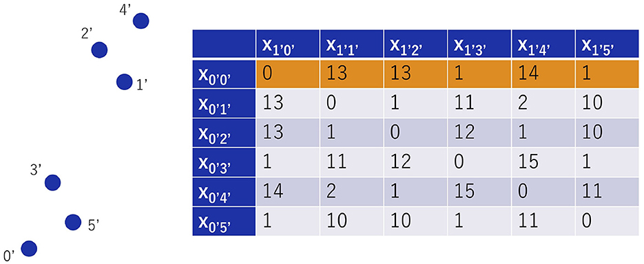
Figure 6. Example when variable indices are not adjacent to each other in nearby cities.

3.2 Partitioning using distance matrix

In the case of the TSP, removing the one-hot condition from the QUBO matrix leaves the objective function part, as shown in Figure 4. In general, the objective function of the QUBO matrix has two parts, one along the diagonal and one on the right, as shown in Figure 7(1). This blocky submatrix is the distance matrix that represents the distance between cities.

Figure 7

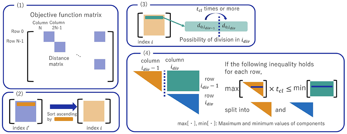
Figure 7. Method of clustering cities from the objective function part of the QUBO matrix.

Figure 7 and the description below show the method of clustering cities and partitioning the problem.

(1) Extract the distance matrix. For an N-city TSP, all distance matrices appearing in the objective function are equal to each other. For example, we can extract the part from row 0 to row N − 1 and from column N to column 2N − 1 as the distance matrix.

(2) If the indices do not line up well, as shown in Figure 6, sort the indices so that the values are in ascending order concerning the rows of the matrix. If the index changes, the variable or QUBO matrix must reflect the change.

(3) Determine in advance the threshold t_cl for clustering. If a component in row 0 (d_0,idiv−1) is t_cl times larger than the component one to its left (d_0,idiv−1), let i_div be the index at which it may be split.

(4) Consider only the upper triangular part of the distance matrix, not including the diagonal components. For each row, check whether all of the components on the right-hand side [d_j,idiv, ⋯d_{j, N−1} (0 ≤ j ≤ i_div−1), the green box of Figure 7(4)] are t_cl times larger than the maximum component on the left-hand side [d_{j, 0}, d_{j, 1}, ⋯ , d_j,idiv−1 (0 ≤ j ≤ i_div−1), the orange triangle of Figure 7(4)] to see if the left-hand part up to i_div−1 column and the right-hand part from i_div column can be partitioned. Once it is verified that the right-hand component is t_cl times larger than the left-hand component, a part of the distance matrix to the i_div−1th row or i_div−1th column [orange triangle of Figure 7(4)] is extracted. The distance information of it is used as the distance matrix of the partitioned problem. In this study, the partitioned problem is called a subproblem. Extract the lower right part from the remaining i_div rows or i_div columns.

(5) Repeat operations (2) to (4) as long as the division is possible.

3.3 Combining subproblem solutions

After the problem is divided into subproblems using the distance matrix, one solves each subproblem as a TSP. However, combining the subproblems' solutions is necessary since the original problem's solution before the division cannot be obtained simply by solving the subproblems. Figure 8 exhibits the method for combining the solutions from solving the subproblems.

(1) TSPs are formulated and solved individually based on the distance matrices of the subproblems (shown by triangles such as yellow and green).

(2) After solving the TSPs for the subproblems, two adjacent cities in each solution of subproblems are randomly selected in each clusters (or one city if there is only one city in a cluster). The selected cities compose the TSP between clusters.

(3) We formulate and solve the TSP for the selected cities. The TSP between these selected cities to determine the order in which to visit the clusters is called the super problem in this study. The distance matrix used in the TSP is constructed from the distance matrix of the original problem before splitting. Since the number of cities is at most twice the number of clusters, the problem should be much easier to solve than before the splitting. In addition, the cities in the same cluster should be in consecutive order.

(4) The solutions of the subproblem TSP are inserted between the two cities of the same cluster in the super problem solution to solve the original TSP. See the explanation of the following and Figure 9 for the method of interpolation.

Figure 8

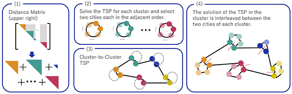
Figure 8. Method to reconstruct the solution of the original problem from the solution of the subproblem.

Figure 9

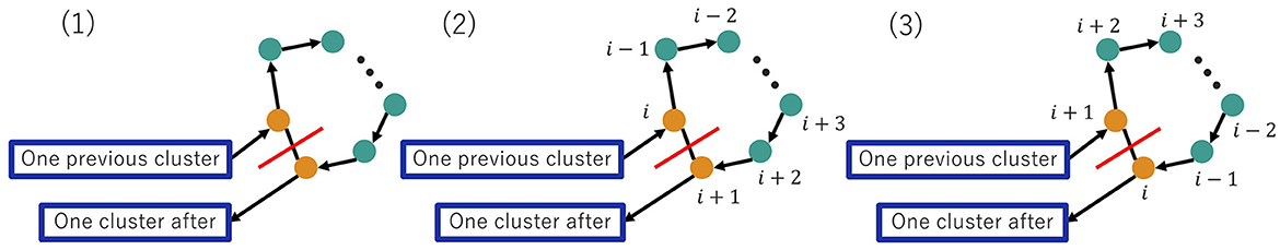
Figure 9. How to insert subproblem solutions between solutions of TSP between clusters (super problem).

After solving the TSP (super problem) for clusters, the solution of the subproblem is inserted into the solution of the super problem to construct the solution of the original problem, as shown in Figure 9.

Suppose the two cities selected from a cluster are the ith and i+1th cities of the solution of the subproblem for the cluster. The ith and i+1th cities correspond to the orange nodes in Figure 9 (1). These two cities are connected to two other clusters, one leading to the previous cluster and the other to the next cluster in the cluster-to-cluster super problem solution.

Since the solution of the original TSP is to go from the previous cluster to the next cluster, the order of visits within each cluster is determined by which city connects to the preceding cluster. In the case of the previous (ith) city connects to the preceding cluster, the order within the cluster appears in the reverse order of the subproblem solution as shown in Figure 9 (2). If the latter (i+1th) city is chosen as the connection, the order within the cluster is the same as the order of the subproblem solution, as shown in Figure 9 (3).

3.4 Local search for inter-cluster connections

The method described in the previous section randomly determines the paths connecting clusters. It may not be easy to obtain the effect of the segmentation. Especially when the number of cities is small, and the Ising machine can reach the optimal solution, the situation is that a better solution can be obtained by not dividing the cities. This section explains a method to find paths connecting clusters by local search.

The method is shown in Figure 10 and described by the following procedure. The local search is performed as a continuation of the stage where the order among clusters is determined by the super problem [Figure 8 (2)].

(1) Now that we know the order of the clusters from the previous steps, the next step is to determine which two cities to choose from each cluster. First, we choose three consecutive clusters in order obtained by the super problem. Since the pathways within each cluster are obtained from the subproblem results, we prepare the variables corresponding to the pathways. For each cluster, the number of pathways equals the number of cities.

(2) Define the distances between paths: four different distances between cities are involved in two paths, and we use the average of the four distances in this article. Construct a QUBO for the three consecutive clusters with a routing scheme that reduces the total distance concerning each cluster, and solve it with an Ising machine. Add a one-hot constraint so the solution has only one path for each cluster.

(3) Pickup of the paths of three consecutive clusters is done for all clusters, splicing them together.

(4) Once the route is determined, two cities are obtained for each cluster. Solve the TSP with at most twice as many cities as the number of clusters as in Figure 8(3). Then, the solution is obtained by interleaving as in Figure 8(4).

Figure 10

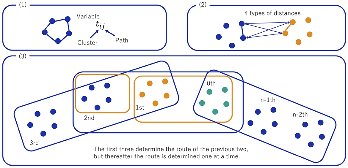
Figure 10. Local search method to find two cities in a cluster.

4 Numerical experiment

4.1 Benchmark problem

In this study, we consider the TSP benchmark problem as shown in Figure 11, where cities exist in clusters, and the optimal solution path is predictable. Each city cluster, distributed in a circle of n clusters, has m cities. Let r be the radius of the circle (called the small circle) in which the cities lie within each cluster, and R is the radius of the circle (called the large circle) in which the clusters line up. The coordinate of the jth (0 ≤ j ≤ m − 1) city in the ith (0 ≤ i ≤ n − 1) cluster is defined as Equation (8).

$\begin{array}{r}(R\cos \left(\frac{2i\pi }{n}\right)+r\cos \left(\frac{2i\pi }{n}+\frac{(2j+1)\pi }{m}-\pi \right),\\ R\sin \left(\frac{2i\pi }{n}\right)+r\sin \left(\frac{2i\pi }{n}+\frac{(2j+1)\pi }{m}-\pi \right)& (8)\end{array}$

To formulate this problem in the QUBO, we define x_{i, jm+k} as the variable whether to visit the kth city in the jth cluster at ith order. When the salesman visits the city at the order, the variable has the value of one x_{i, jm+k} = 1. On the other hand, when the salesman does not visit the city at the order, x_{i, jm+k} = 0. Here, 0 ≤ i ≤ mn − 1, 0 ≤ j ≤ n−1, and 0 ≤ k ≤ m − 1. The formulation of the Hamiltonian is the same as that of the TSP for mn cities, and one can get it by rewriting N as mn in Equations (5–7).

Figure 11

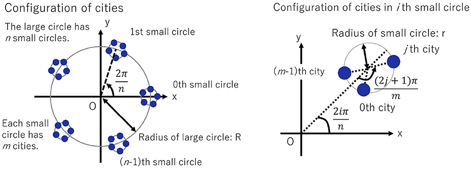
Figure 11. Distribution of cities in the benchmark problem.

In this study, we solve the TSP for 36, 64, and 100 cities, corresponding to m = n = 6, 8, and 10, respectively. The threshold of distance multiplicity in clustering t_cl is t_cl = 2, the radius of the small circle is r = 1, and the radius of the large circle is $R=\frac{1.1(t_{cl}+1)r}{sin(\pi /n)}$. Here, the radius of the large circle is determined so that each small circle can exist as a cluster.

The optimal solution of the TSP for cities represented in Figure 11 is to visit each small circle in turn through the neighboring circles. For each small circle, the shortest path visits the 0th city, the first city, ⋯ , and the (m − 1)th city in sequence. For the paths between the small circles, the shortest path goes from the (m − 1)th city of the kth small circle to the 0th city of the (k+1)th small circle. Finally, the shortest path is from the (m − 1)th city of the (n − 1)th small circle to the 0th city of the 0th small circle.

4.2 Coefficient parameter dependence

When using an Ising machine, the products of the coefficient parameters and the polynomials representing the constraints and objective functions are the terms in the input Hamiltonian. The magnitude of the coefficient parameters of the constraints and the objective functions affects the ease of obtaining an optimal solution that satisfies the constraints. In this section, we examine how the solutions obtained by the two proposed partitioning methods, one of which is a method to randomly determine the paths between clusters and the other of which is a method that determines the paths between clusters by local search, differ in terms of quality from the solution obtained by solving the problem as is while varying the coefficient parameters.

We introduce C_C and C_O as the coefficient parameters. The parameter C_C is a coefficient parameter on the Hamiltonian H_C, including the two one-hot constraints (corresponding to the sum of Equations 5, 6). The parameter C_O corresponds to a coefficient on the Hamiltonian H_O of the objective function representing the total distance traveled (corresponding to Equation 7). We set C_C and C_O as Equation (9), where p is the coefficient parameter and max(d_ij) is the maximum distance between cities and solve the Hamiltonian C_CH_C+C_OH_O of TSPs.

$\begin{array}{ll}{C}_C=p\times \text{max}(d_{ij}),C_O=1.& (9)\end{array}$

We evaluate the proposed methods using NEC's Vector Annealing (Takano et al., 2019; NEC Corporation, 2022b) (version 2.0.1), which is based on simulated annealing, on an NEC SX-Aurora TSUBASA hardware with Intel Xeon Gold 6226 (2.7 GHz) and NEC Vector Engine Type 20B, as the Ising machine. The settings required for the Vector Annealing calculations in this experiment are as follows: “num_sweeps," a parameter that controls the number of calculation steps, is set to 100. “vector_mode," a parameter for prioritizing between speed and accuracy, is set to “accuracy" for accuracy. “beta_range," which decide the temperature parameter for simulated annealing, is set to the default value.

We also use the “flip option" function of Vector Annealing, which allows the annealing calculations to be solved while considering constraints. In this study, we use the “One hot" constraint function that considers one-hot conditions and the “Fixed spin" constraint function that fixes the values of variables. The “One hot" constraint function includes all one-hot conditions in TSP. For the “Fixed spin" constraint function, the first city to be visited is the city with the youngest index, and thus, the variables to be determined are fixed. For example, when the variable is defined as x_ij (0 ≤ i, j ≤ N − 1), the “Fixed spin" constraint function fixes the variables as x₀₀ = 1, x_i0 = x_0i = 0 (1 ≤ i ≤ N − 1).

The results of solving the TSP benchmark problem for m = n = 6, 8, 10 as is and using the two division methods proposed in this study while varying the coefficient parameters are shown in Figure 12. In each panel, the blue plots and lines represent the results of solving the problem without the division (“Orig"). The orange plots and lines represent the results obtained using the division method to randomly determine the paths between clusters proposed in this study (“Div"). The green plots and lines are for the division method that determines the paths between clusters by local search (“Lcl"). The filled round plots and dashed circle plots represent the average length of the TSP paths for the solutions that satisfy all the constraints. We have 100 solutions of each case. A filled circle indicates that all 100 solutions satisfy the constraints (“Sat"), while a dashed circle plot indicates that some solutions do not. Cross plots represent the shortest path lengths. Vertical bars on the round plots indicate the standard deviation. There is no plot if any solutions that satisfy the constraints cannot be obtained. The path length in the optimal solution is the black dashed line extending horizontally across the graph. We calculate the cases from p = 0.1 to p = 2.0 in increments of 0.1, but for the p = 0.1 case, no solution satisfies the constraints except for one result. More specific distances and computation time information are included in Supplementary material.

Figure 12

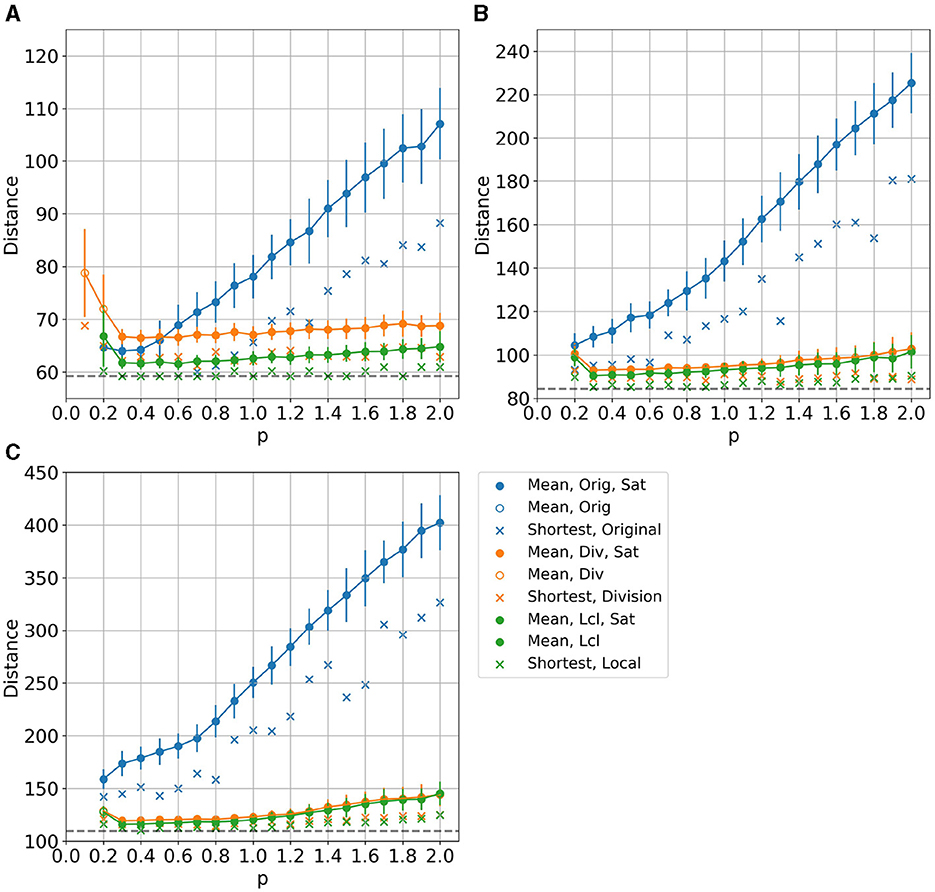
Figure 12. Coefficient parameter p dependence of the distance for the (A) 36, (B) 64, and (C) 100 cities benchmark problem.

The overall trend of the results, particularly noticeable when the number of cities is large, is that the two proposed division methods yield solutions closer to the optimal solution than the case solved without division, regardless of the coefficient parameter p. On the other hand, when solving without division, it is necessary to determine the coefficients of the objective function and the constraint part of the Hamiltonian as the values near the boundary between satisfying and not satisfying the constraint conditions, e.g., p = 0.2.

Let us discuss the problem for the individual number of cities. In the case of m = n = 6 (Figure 12A), the solutions obtained by solving the problem as is are sometimes better than those obtained by the splitting. The average distance is smaller when solving as is than when splitting at p = 0.2. The situation where the solution is better if solved without splitting is because the Ising machine used is capable to solve the problem as is.

However, adjusting the parameters is essential, and as p increases, the average of the distances when solving as is becomes larger and larger. On the other hand, when solving by splitting, the average distance does not increase much as p increases. This result indicates that the method of solving by splitting is more robust than the method of solving as is in terms of adjusting the parameters of the constraints.

In addition, in the case of splitting, the local search method of path connection between clusters gives better results than that of random connection. Due to local search, we can find better ways to connect clusters.

The solutions of the partitioning method with random choices produces satisfied the constraint condition for p = 0.1. The constraint conditions are satisfied in five out of 100 cases, while the other methods do not satisfy the constraint condition for p = 0.1. This is related to the division resulting in a simpler TSP than the original problem, making it easier to satisfy the constraint conditions. In addition, the fact that the method with local search for paths between clusters does not obtain the result for p = 0.1 is because the method with local search solves more TSPs than the method with random choices of paths between clusters, which makes the problem less likely to satisfy the constraint condition for all TSPs.

In the case of m = n = 8, 10 shown in Figures 12B, C, the lengths of the distances significantly differ when solving the problem as is or when splitting the problem. This may be because the number of cities is larger, making the problem more difficult, but the problem becomes simpler by dividing the cities into clusters. This is particularly evident in the results of m = n = 10. In the results obtained by the two proposed methods, the average value and standard deviation of the distances are larger at p = 0.2 when the constraint begins to be satisfied than those at p = 0.3. On the other hand, when solved as is, the mean value and standard deviation of the distances are smaller when p = 0.2 than when p = 0.3.

4.3 “num_sweeps" dependence

Next, we show the dependence of the solution distance of the TSP on the value of “num_sweeps," which is a parameter of Vector Annealing and related to the Monte Carlo step of simulated annealing. When num_sweeps becomes larger, the solution is likely to be closer to the optimal solution. For smaller problems, a solution close to the optimal solution can be obtained without increasing num_sweeps too much.

Here, for each of the cases of m = n = 6, 8, and 10 without and with splitting, respectively, the results are computed with num_sweeps set to 10, 30, 50, 100, and 200, with the coefficient parameter p which gives the shortest distance of the TSP solution in the previous section. Note that the results when num_sweeps is 100 are the same as those in the computation of Figure 12. If more than one parameters p give the shortest distance, the p with the highest number of times for the shortest distance is adopted. Furthermore, we use the p with the shortest average distance in case of the same number of times. The following are the specific values. p = 0.4 (Orig), p = 0.7 (Div), p = 0.6 (Lcl) for m = n = 6; p = 0.2 (Orig), p = 1.3 (Div), p = 0.3 (Lcl) for m = n = 8; p = 0.2 (Orig), p = 0.8 (Div), p = 0.4 (Lcl) for m = n = 10.

The results are shown in Figure 13. Each case of the number of cities and the parameter num_sweeps has 100 computed results, and solutions that satisfied the constraints are obtained, except for the case where num_sweeps was set to 10 in the results for m = n = 8, 10 without splitting.

Figure 13

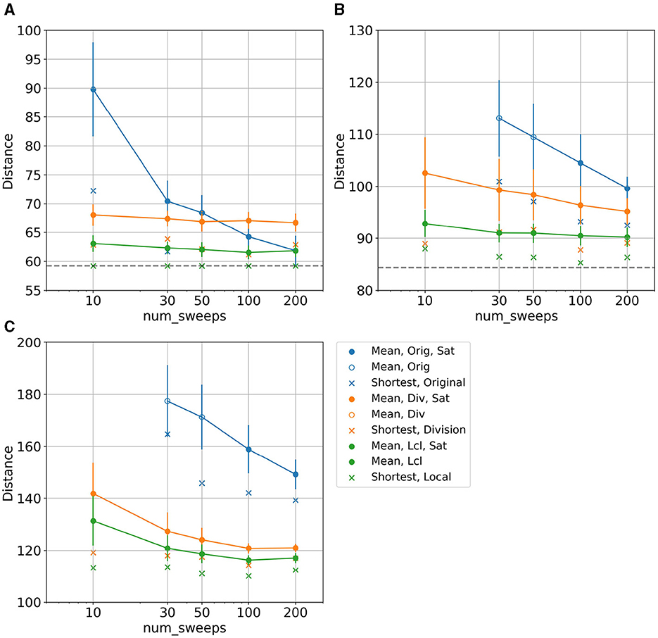
Figure 13. Dependence of the distance on the parameter num_sweeps associated with the Monte Carlo step of simulated annealing. The legend is the same as in Figure 12, and each plot uses 100 calculations. (A) 36 cities. (B) 49 cities. (C) 100 cities.

These results show that in the case of no partitioning, the distance becomes shorter as the number of num_sweeps increases. The constraints are more likely to be satisfied as shown in Figures 13B, C, in which we obtained a solution that does not satisfy the constraint conditions in case of small num_sweeps values, but as increasing num_sweeps, all 100 solutions satisfy the constraint condition. In addition, since the mean value of the distance does not converge in the results without splitting, a shorter distance may be obtained by increasing the number of num_sweeps.

On the other hand, in the case of splitting, the distance of the path does not depend on num_sweeps very much. This is because the TSPs solved in the case of splitting are small, and thus, a solution close to the optimal solution is obtained even if num_sweeps is small. Thus, even a large-scale problem with many variables can be treated as multiple small-scale problems by dividing the TSP and solved without increasing num_sweeps.

More specific distances and computation time information are included in Supplementary material.

5 Discussion

5.1 Limitation of proposed method

In Section 4, we demonstrated the usefulness of the proposed method by solving benchmark problems in which the effects of clustering are easy to see. In this section, we discuss the limitations of the proposed method and a comparison with 2-opt, which is often used when solving TSPs, with particular attention to problem splitting.

In this study, we propose a method that automatically partitions from a given QUBO matrix without being aware of the distribution of cities, but only if the breaks in the clusters are so clear that it is apparent that the cities can be clustered when one looks at the distribution of cities. This is because even if a candidate city for a break of clusters is found from the distance matrix in step (3) of Figure 7, it turns out in step (4) of Figure 7 that there is no break of clusters because that city is close to a city outside the clusters that have been constructed so far. For example, distributions with no structure in two dimensions, such as evenly or randomly distributed cities, cannot be divided, and the proposed method cannot be applied.

In addition, the proposed method cannot be used for one-dimensional continuous distributions. For example, the proposed method is ineffective for cities distributed in a linear, ring, or Figure 8 pattern, etc., as the cluster breaks cannot be determined. However, constructing clusters by increasing the number of elements one by one, such as agglomerative hierarchical clustering, may be effective in such cases. It is also noted that although the city distributions solved by the numerical experiment are ring-shaped, the proposed method is effective because the small circles are sufficiently far from each other and can be regarded as clusters.

Next, we compare the proposed method in this article with 2-opt concerning the size of the solution space and discuss the pros and cons of the proposed method over 2-opt. 2-opt is a well-known local search algorithm for TSP, where it swaps two paths for a given circuit if the distance between them becomes shorter.

First, let us consider the difference in the size of the solution space explored by the Ising machine and 2-opt in TSP. When the number of cities is N, the number of feasible circuits is (N − 1)!/2. Since 2-opt only searches for feasible circuits, the number of elements in the solution space to be searched is the same as that of feasible circuits, (N − 1)!/2.

On the other hand, in the formulation in this article of TSPs for the Ising machine, N² binary variables are prepared, so the number of elements in the solution space to be searched is 2^N2. Of these, the number of solutions satisfying the two-way one-hot condition is N!. The two-way one-hot condition is rather severe, and as the number of cities increases when solving a TSP with the Ising machine, the constraint becomes difficult to satisfy.

The number of elements in the solution space indicates that as N increases, the solution space explored by the Ising machine rapidly becomes larger than the solution space explored by 2-opt.

When solving a TSP as it is, if the Ising machine's performance in terms of solution speed and solution quality is so high that the solution space size can be overcome, then it can be said to have an advantage over 2-opt. However, such a situation is not obvious. One advantage of Ising machines would be that a globally optimal solution can be reached if the computation time is long enough for simulated annealing (Geman and Geman, 1984) and quantum annealing (Morita and Nishimori, 2008).

On the other hand, if TSPs can be solved for each cluster of cities using the proposed method, the size of the solution space will be smaller, which may have advantages over 2-opt in terms of solution space size. For example, in the case where m clusters exist, and n cities exist in a cluster, the number of elements in the solution space of a cluster is 2ⁿ² when solving with the Ising machine, and the number of elements in the solution space of the problem of finding paths between clusters is 2^(2m)2.

These solution spaces would be smaller than the original TSP, of which the number of cities is N > m, n. The solution space of each solution would be smallest when $m,n\simeq \sqrt{N}$.

However, this situation is limited to cases where cities are distributed in clusters, and the number of cities in a cluster and the number of clusters are not too large. If the number of clusters m or the number of cities n in a cluster is large, e.g., 2ⁿ² ≫ (N − 1)!/2, then there is no advantage to the proposed method.

In addition, although the proposed method uses Ising machines to find a path after partitioning the problem, it is possible to replace Ising machines with 2-opt. Strictly speaking, we can claim the merit of the proposed method only for problems with clusters where 2-opt would result in a locally optimal path. For such problems, using simulated or quantum annealing to find paths has the advantage of not falling into the local optimum if the computation time is as long as necessary.

5.2 Application to other problems

The method proposed in this study can be applied to problems with two-way one-hot conditions other than TSP. As application examples, we deal with the problems of ordering things, which we call “ordering problems," and the quadratic assignment problems (QAPs).

5.2.1 Ordering problem

The ordering problem appears, for example, when choosing the order in which products are produced. In a factory that produces many types of products with the same equipment, it is necessary to change the preparation of materials and parts and the settings of manufacturing equipment when changing the products to be produced, and these preparation and settings take time. Since the time required for preparation and setting changes depends on the combination of products before and after they are manufactured, it is necessary to determine the order in which the preparation time is reduced to utilize the manufacturing line efficiently.

The ordering problem can be formulated as QUBO with two-way one-hot constraints, and the objective function is almost the same as in TSP. We define the corresponding binary variable x_ij ∈ {0, 1}, which means that ith manufactured product is j (x_ij = 1) or not (x_ij = 0). The Hamiltonian has elements of Equations (10) and (11), where c_ij is the preparation time it takes to manufacture product j after manufacturing product i.

$\begin{array}{ll}{H}_C={\displaystyle \sum _{i=0}^{N-1}}{\left({\displaystyle \sum _{j=0}^{N-1}}{x}_{ij}-1\right)}^2+{\displaystyle \sum _{j=0}^{N-1}}{\left({\displaystyle \sum _{i=0}^{N-1}}{x}_{ij}-1\right)}^2& (10)\end{array}$

$\begin{array}{ll}{H}_O={\displaystyle \sum _{i=0}^{N-2}}{\displaystyle \sum _{j\ne k}}{c}_{jk}{x}_{ij}{x}_{i+1,k}& (11)\end{array}$

Since the cost of changing the product to be manufactured can be regarded as the distance of the TSP, the matrix of the cost of changing the product (hereafter referred to as the cost matrix) can be arranged in the QUBO matrix as the distance matrix of the TSP. However, the TSP requires the order of cities to travel around, visiting all cities to be visited, and returning to the city from which it started. The difference is that the ordering problem produces all the products that need to be manufactured and does not require the first product to be manufactured again. Therefore, in the QUBO matrix of the objective function of the ordering problem, the upper right part of the matrix that exists in the case of TSP does not exist, as shown in Figure 14.

Figure 14

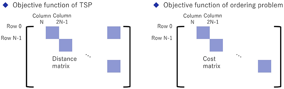
Figure 14. Differences in the structure of the objective function part of the QUBO matrix in the TSP (left) and the ordering problem (right).

Although there are differences in the objective function part of the QUBO matrix, the ordering problem can be divided and solved similarly to TSP. In the objective function part of the QUBO matrix, the cost matrix to change the product appears with the first index of the variable shifted by one, and they are all identical. When dividing, we can choose only one of the cost matrices and divide it as we do for the TSP (Figure 7). Based on each divided cost matrix, the original ordering problem is solved as multiple subproblems. The subproblem can then be solved as a TSP by arranging the divided cost matrix in the QUBO matrix of the objective function in block form as in the TSP. This is because, in the proposed method for solving the TSP, the solution of the subproblem is used to find the order of cities to visit by cutting through the path of two neighboring cities.

Next, the first and last products in each subproblem are used to order among the clustered product groups as a super problem. Although the super problem of a TSP is constructed from the distance matrix in the proposed method, the ordering problem is not a problem in determining the cycle of manufacturing, so post-processing is required to obtain the solution to the original ordering problem. We can solve the ordering problem by cutting out the most costly switching. In the solution for the original ordering problem, the item immediately after the cutout is set as the first in the order, and the item immediately before the cutout is set as the last.

As for the application limits of the proposed method in the ordering problem, a situation is similar to that of TSPs. It is impossible to split the problem unless the break of the product groups in the cost matrix is clear. Even if a candidate product for a break of clusters is found from the cost matrix, it cannot be the border of the cluster if the switching cost with the product outside the cluster is small.

5.2.2 Quadratic assignment problem

The quadratic assignment problem (QAP) is another problem with the two-way one-hot constraint, to which our proposed method can be applied. QAPs ask which factory should be built on which site to minimize the cost when building a factory on a site. The cost is expressed as the product of the flow, representing the amount of materials exchanged between factories, and the distance between sites. The formulation into the QUBO has a binary variable x_ij representing whether factory i is built on site j, and the Hamiltonian has elements of Equations (12) and (13), where f_ik represents the flow between factories i, k and d_jl represents the distance between sites j, l.

$\begin{array}{ll}{H}_C={\displaystyle \sum _{i=0}^{N-1}}{\left({\displaystyle \sum _{j=0}^{N-1}}{x}_{ij}-1\right)}^2+{\displaystyle \sum _{j=0}^{N-1}}{\left({\displaystyle \sum _{i=0}^{N-1}}{x}_{ij}-1\right)}^2& (12)\end{array}$

$\begin{array}{ll}{H}_O={\displaystyle \sum _{i,j,k,l=0}^{N-1}}{\displaystyle \sum _{j\ne k}}{f}_{ik}{d}_{jl}{x}_{ij}{x}_{kl}& (13)\end{array}$

For a TSP or an ordering problem, one of the indices of the variables represents the order. Only one type of cost, e.g., the distance between cities, needs to be considered in these problems. On the other hand, QAPs are more complex than TSPs or ordering problems because it requires the consideration of two factors: factories and sites. In the objective function part of the QUBO matrix of a QAP, the cost matrices, which are the products of the distance matrix between factories and the flows, appear in blocks. However, each block differs by a constant factor and exists where the first and second indices of the variable are shifted unlike TSPs and the ordering problems as shown in Figure 15A.

Figure 15

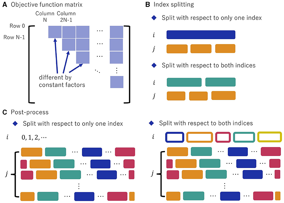
Figure 15. Structures of the QUBO matrix of a QAP and how to post-process it using these properties. (A) The objective function part of the QUBO matrix of a QAP. (B) In QAPs, there are cases where clustering is possible for only one of the two indices (top panel) and cases where clustering is possible for two indices (bottom panel). (C) Unlike TSPs and the ordering problems, the variables for QAPs have two meaningful indices to consider, so it would be fruitful to search for a better solution by switching the indices after solving the problem as TSP.

Nevertheless, clustering regarding distance is possible because the cost matrices are constant multiples of the distance matrix by the values of flows. Each block is considered a distance matrix in the TSP, and these “distance matrices" are used to cluster the variables. They represent the product of the distance matrix between sites and a particular flow. Since the non-zero components of the “distance matrices" differ only by a constant factor, we can use a single “distance matrix" to cluster the sites by regarding them as cities. One can partition sites into clusters, which correspond to the second index of variables.

In TSPs and the ordering problems, only one of the two indices is clustered. In contrast, in QAPs, there are cases where clustering is possible for only one of the two indices (top panel) and cases where clustering is possible for two indices (bottom panel). Clustering is also possible for flows by reordering the indices (x_ij→x_ji). As in the case of clustering the sites, the products of the flow matrix and a distance appear in the objective function part of the QUBO matrix in the form of a block, so the next step is to cluster the factories by considering constant multiple of the flow matrix as the “distance matrix." If only one of the indices can be clustered, the clustered index should be the second.

Suppose clustering is possible concerning distance or flow (Figure 15B), there may be a possibility that the solution obtained by rearranging the index of clusters and dividing it into clusters as a TSP may be a good solution for QAPs. Here, we propose a method to solve the problem as a TSP, although it is a QAP problem. Using the “distance matrix" used for the clustering and considering the factories or sites as cities in TSPs, the order of the indices of the variables in the clusters is determined by solving the TSP for each cluster. Once the order is determined for each cluster, the order between clusters is determined by taking two adjacent factories or sites in order in the TSP solution for each cluster, defining the distance between the clusters by using the original “distance matrix," and solving the TSP. The order of the factories of sites in the clusters is then interleaved to solve the original problem.

However, unlike TSPs, QAPs have two indices to consider, so it may be better to check the post-processed solutions as solutions rather than just using the solution solved as a TSP. The obtained solution is cycled with the second index, and multiple solutions are compared. For example, if the solution that x_0i0 = x_1i1 = ⋯ = x_{N − 1,iN−1} = 1 and the other variables x_ij have the value 0 are obtained, one need to consider the solutions with the first index shifted, which are cycled from x_1i0 = x_2i1 = ⋯ = x_N−1,iN−2 = x_0,iN−1 = 1, others = 0 to x_N−1,i0 = x_0i1 = ⋯ = x_N−2,iN−1 = 1, others = 0, which is shown as the left part of Figure 15C. After comparing the solution quality of all solutions, the best solution should be considered as the solution. At this time, it is also essential to cluster and redefine the other index that is not clustered in the TSP, if clustering is possible (the right part of Figure 15C). This is because by clustering the other index, we can expect to increase the number of elements for which the product of distance and flow is smaller.

However, the proposed method's effectiveness is considered even more limited in QAP than in TSP. When the proposed method is applied to TSP, all the indices are equivalent in terms of order, so it is effective only if the distribution of cities can be clustered. On the other hand, in QAP, there are two perspectives, factories and site, and even if the proposed method is optimized with respect to the site using the TSP approach, the optimization does not necessarily work well concerning flow.

6 Summary

In this article, we have proposed a method of problem partitioning from the QUBO input of a traveling salesman problem (TSP) with the two-way one-hot constraint, in which even users unfamiliar with the Ising machines, who will likely let the Ising machine solve the problem as it is, can take advantage of the problem partitioning. Using the objective function part of the QUBO matrix of the TSP, which can be brought out because the two-way one-hot constraint has a characteristic structure in a QUBO matrix, we partition the cities into clusters and solve TSPs between cities in each cluster (subproblems) and a TSP between clusters (super problem). It is found that solving the TSP between cities in clusters and the TSP between clusters provides a better solution than solving the problem as it is, especially for TSPs that are so large that the Ising machine itself cannot provide an optimal solution. Furthermore, when solving TSPs between clusters, it is also found that determining the cities that serve as joint cities between clusters by local search yields a better solution than when the bond cities are chosen at random. Our proposed method can be also applied to the problem of ordering things and the quadratic assignment problem, which have the two-way one-hot conditions.

Data availability statement

The original contributions presented in the study are included in the article/Supplementary material, further inquiries can be directed to the corresponding author.

Author contributions

AY: Writing – original draft.

Funding

The author(s) declare financial support was received for the research, authorship, and/or publication of this article. This article was based on results obtained from a project, JPNP16007, commissioned by the New Energy and Industrial Technology Development Organization (NEDO), Japan.

Acknowledgments

The author thanks R. Miyazaki, T. Nishimura, and F. Takano for helpful comments on the manuscript. The author also thanks H. Chishima for discussion of the early stages of this study.

Conflict of interest

AY is employed by NEC Corporation and Vector Annealing is a product of NEC Corporation. A patent application is pending for this research.

Publisher's note

All claims expressed in this article are solely those of the authors and do not necessarily represent those of their affiliated organizations, or those of the publisher, the editors and the reviewers. Any product that may be evaluated in this article, or claim that may be made by its manufacturer, is not guaranteed or endorsed by the publisher.

Supplementary material

The Supplementary Material for this article can be found online at: https://www.frontiersin.org/articles/10.3389/fcomp.2024.1285244/full#supplementary-material

References

Abbott, A. A., Calude, C. S., Dinneen, M. J., and Hua, R. (2019). A hybrid quantum-classical paradigm to mitigate embedding costs in quantum annealing. Int. J. Quantum Inf. 17:1950042. doi: 10.1142/S0219749919500424

Crossref Full Text | Google Scholar

Abel, S., Chancellor, N., and Spannowsky, M. (2021). Quantum computing for quantum tunneling. Phys. Rev. D 103:016008. doi: 10.1103/PhysRevD.103.016008

Crossref Full Text | Google Scholar

Atobe, Y., Tawada, M., and Togawa, N. (2021). Hybrid annealing method based on subQUBO model extraction with multiple solution instances. IEEE Trans. Comput. 71, 2606–2619. doi: 10.1109/TC.2021.3138629

Crossref Full Text | Google Scholar

Bando, Y., Susa, Y., Oshiyama, H., Shibata, N., Ohzeki, M., Gómez-Ruiz, F. J., et al. (2020). Probing the universality of topological defect formation in a quantum annealer: Kibble-Zurek mechanism and beyond. Phys. Rev. Res. 2:033369. doi: 10.1103/PhysRevResearch.2.033369

Crossref Full Text | Google Scholar

Bauckhage, C., Brito, E., Cvejoski, K., Ojeda, C., Sifa, R., Wrobel, S., et al. (2018). “Ising models for binary clustering via adiabatic quantum computing,” in Energy Minimization Methods in Computer Vision and Pattern Recognition: 11th International Conference, EMMCVPR 2017, Venice, Italy, October 30-November 1, 2017, Revised Selected Papers 11 (Cham: Springer), 3–17. doi: 10.1007/978-3-319-78199-0_1

Crossref Full Text | Google Scholar

Bernal, D. E., Booth, K. E., Dridi, R., Alghassi, H., Tayur, S., Venturelli, D., et al. (2020). “Integer programming techniques for minor-embedding in quantum annealers,” in Integration of Constraint Programming, Artificial Intelligence, and Operations Research: 17th International Conference, CPAIOR 2020, Vienna, Austria, September 21-24, 2020, Proceedings 17 (Cham: Springer), 112–129. doi: 10.1007/978-3-030-58942-4_8

Crossref Full Text | Google Scholar

Bian, Z., Chudak, F., Israel, R. B., Lackey, B., Macready, W. G., Roy, A., et al. (2016). Mapping constrained optimization problems to quantum annealing with application to fault diagnosis. Front. ICT 3:14. doi: 10.3389/fict.2016.00014

Crossref Full Text | Google Scholar

Booth, M., Reinhardt, S., and Roy, A. (2017). Partitioning optimization problems for hybrid classical/quantum execution. Available online at: https://docs.ocean.dwavesys.com/projects/qbsolv/en/latest/_downloads/bd15a2d8f32e587e9e5997ce9d5512cc/qbsolv_techReport.pdf (accessed August 21, 2023).

Google Scholar

Borle, A., and McCarter, J. (2019). “On post-processing the results of quantum optimizers,” in International Conference on Theory and Practice of Natural Computing (Cham: Springer), 222-233. doi: 10.1007/978-3-030-34500-6_16

Crossref Full Text | Google Scholar

Chancellor, N. (2017). Modernizing quantum annealing using local searches. New. J. Phys. 19:023024. doi: 10.1088/1367-2630/aa59c4

Crossref Full Text | Google Scholar

Chancellor, N. (2023). Modernizing quantum annealing II: genetic algorithms with the inference primitive formalism. Nat. Comput. 22, 737–752. doi: 10.1007/s11047-022-09905-2

Crossref Full Text | Google Scholar

D-Wave Quantum Inc. (2021). QBSOLV. Available online at: https://docs.ocean.dwavesys.com/projects/qbsolv/en/latest/ (accessed August 1, 2023.).

Google Scholar

D-Wave Quantum Inc. (2023a). D-wave Hybrid. Available online at: https://docs.ocean.dwavesys.com/projects/hybrid/en/latest/ (accessed August 1, 2023.).

Google Scholar

D-Wave Quantum Inc. (2023b). The most connected and powerful quantum computer built for business. Available online at: https://www.dwavesys.com/solutions-and-products/systems/ (accessed August 1, 2023.).

Google Scholar

Feld, S., Roch, C., Gabor, T., Seidel, C., Neukart, F., Galter, I., et al. (2019). A hybrid solution method for the capacitated vehicle routing problem using a quantum annealer. Front. ICT 6:13. doi: 10.3389/fict.2019.00013

Crossref Full Text | Google Scholar

Gaidai, I., Babikov, D., Teplukhin, A., Kendrick, B. K., Mniszewski, S. M., Zhang, Y., et al. (2022). Molecular dynamics on quantum annealers. Sci. Rep. 12:16824. doi: 10.1038/s41598-022-21163-x

PubMed Abstract | Crossref Full Text | Google Scholar

Geman, S., and Geman, D. (1984). Stochastic relaxation, gibbs distributions, and the bayesian restoration of images. IEEE Trans. Pattern Anal. Mach. Intell. PAMI-6, 721–741. doi: 10.1109/TPAMI.1984.4767596

PubMed Abstract | Crossref Full Text | Google Scholar

Irie, H., Liang, H., Doi, T., Gongyo, S., and Hatsuda, T. (2021). Hybrid quantum annealing via molecular dynamics. Sci. Rep. 11:8426. doi: 10.1038/s41598-021-87676-z

PubMed Abstract | Crossref Full Text | Google Scholar

Izawa, S., Kitai, K., Tanaka, S., Tamura, R., and Tsuda, K. (2022). Continuous black-box optimization with an ising machine and random subspace coding. Phys. Rev. Res. 4:023062. doi: 10.1103/PhysRevResearch.4.023062

Crossref Full Text | Google Scholar

Jain, S. (2021). Solving the traveling salesman problem on the D-wave quantum computer. Front. Phys. 9:760783. doi: 10.3389/fphy.2021.760783

Crossref Full Text | Google Scholar

Kanamaru, S., Kawamura, K., Tanaka, S., Tomita, Y., and Togawa, N. (2021). Solving constrained slot placement problems using an ising machine and its evaluations. IEICE Trans. Inf. Syst. E104-D, 226–236. doi: 10.1587/transinf.2019EDP7254

PubMed Abstract | Crossref Full Text | Google Scholar

King, J., Yarkoni, S., Nevisi, M. M., Hilton, J. P., and McGeoch, C. C. (2015). Benchmarking a quantum annealing processor with the time-to-target metric. arXiv [Preprint]. arXiv:1508.05087. doi: 10.48550/arXiv.1508.05087

Crossref Full Text | Google Scholar

King, J., Yarkoni, S., Raymond, J., Ozfidan, I., King, A. D., Nevisi, M. M., et al. (2019). Quantum annealing amid local ruggedness and global frustration. J. Phys. Soc. Jpn. 88:061007. doi: 10.7566/JPSJ.88.061007

PubMed Abstract | Crossref Full Text | Google Scholar

Kitai, K., Guo, J., Ju, S., Tanaka, S., Tsuda, K., Shiomi, J., et al. (2020). Designing metamaterials with quantum annealing and factorization machines. Phys. Rev. Res. 2:013319. doi: 10.1103/PhysRevResearch.2.013319

Crossref Full Text | Google Scholar

Kumagai, M., Komatsu, K., Takano, F., Araki, T., Sato, M., Kobayashi, H., et al. (2021). An external definition of the one-hot constraint and fast QUBO generation for high-performance combinatorial clustering. Int. J. Netw. Comput. 11, 463–491. doi: 10.15803/ijnc.11.2_463

Crossref Full Text | Google Scholar

Liu, X., Ushijima-Mwesigwa, H., Mandal, A., Upadhyay, S., Safro, I., Roy, A., et al. (2022). Leveraging special-purpose hardware for local search heuristics. Comput. Optim. Appl. 82, 1–29. doi: 10.1007/s10589-022-00354-2

Crossref Full Text | Google Scholar

Lubinski, T., Coffrin, C., McGeoch, C., Sathe, P., Apanavicius, J., Neira, D. E. B., et al. (2023). Optimization applications as quantum performance benchmarks. arXiv [Preprint]. arXiv:2302.02278. doi: 10.48550/arXiv.2302.02278

Crossref Full Text | Google Scholar

Matsumoto, N., Hamakawa, Y., Tatsumura, K., and Kudo, K. (2022). Distance-based clustering using QUBO formulations. Sci. Rep. 12:2669. doi: 10.1038/s41598-022-06559-z

PubMed Abstract | Crossref Full Text | Google Scholar

Mniszewski, S. M., Dub, P. A., Tretiak, S., Anisimov, P. M., Zhang, Y., Negre, C. F., et al. (2021). Reduction of the molecular hamiltonian matrix using quantum community detection. Sci. Rep. 11:4099. doi: 10.1038/s41598-021-83561-x

PubMed Abstract | Crossref Full Text | Google Scholar

Mori, N., and Furukawa, S. (2023). Quantum annealing for the adjuster routing problem. Front. Phys. 11:1129594. doi: 10.3389/fphy.2023.1129594

Crossref Full Text | Google Scholar

Morita, S., and Nishimori, H. (2008). Mathematical foundation of quantum annealing. J. Math. Phys. 49:125210. doi: 10.1063/1.2995837

Crossref Full Text | Google Scholar

Mukai, K., and Kudo, K. (2021). Pattern formation simulated by an Ising machine. J. Phys. Soc. Jpn. 90:025004. doi: 10.7566/JPSJ.90.025004

PubMed Abstract | Crossref Full Text | Google Scholar

NEC Corporation (2022a). NEC and NEC Fielding introduce a delivery planning system for maintenance parts utilizing quantum computing technology. Available online at: https://www.nec.com/en/press/202209/global_20220909_03.html (accessed August 1, 2023).

Google Scholar

NEC Corporation (2022b). NEC to launch simulated annealing service with up to 300,000 bits. Available online at: https://www.nec.com/en/press/202208/global_20220829_01.html (accessed August 1, 2023).

Google Scholar

NEC Corporation (2023). NEC and NEC Platforms introduce a production planning system for ICT equipment utilizing quantum computing technology at four NEC Platforms business sites. Available online at: https://www.nec.com/en/press/202301/global_20230120_02.html (accessed August 1, 2023).

Google Scholar

Neukart, F., Compostella, G., Seidel, C., von Dollen, D., Yarkoni, S., Parney, B., et al. (2017). Traffic flow optimization using a quantum annealer. Front. ICT 4:29. doi: 10.3389/fict.2017.00029

PubMed Abstract | Crossref Full Text | Google Scholar

Nishimura, N., Tanahashi, K., Suganuma, K., Miyama, M. J., and Ohzeki, M. (2019). Item listing optimization for E-commerce websites based on diversity. Front. Comput. Sci. 1:2. doi: 10.3389/fcomp.2019.00002

Crossref Full Text | Google Scholar

Ohzeki, M. (2020). Breaking limitation of quantum annealer in solving optimization problems under constraints. Sci. Rep. 1:3126. doi: 10.1038/s41598-020-60022-5

PubMed Abstract | Crossref Full Text | Google Scholar

Ohzeki, M., Miki, A., Miyama, M. J., and Terabe, M. (2019). Control of automated guided vehicles without collision by quantum annealer and digital devices. Front. Comput. Sci. 1:9. doi: 10.3389/fcomp.2019.00009

Crossref Full Text | Google Scholar

Okada, S., Ohzeki, M., and Taguchi, S. (2019a). Efficient partition of integer optimization problems with one-hot encoding. Sci. Rep. 9:13036. doi: 10.1038/s41598-019-49539-6

PubMed Abstract | Crossref Full Text | Google Scholar

Okada, S., Ohzeki, M., Terabe, M., and Taguchi, S. (2019b). Improving solutions by embedding larger subproblems in a D-wave quantum annealer. Sci. Rep. 9:2098. doi: 10.1038/s41598-018-38388-4

PubMed Abstract | Crossref Full Text | Google Scholar

Oku, D., Tawada, M., Tanaka, S., and Togawa, N. (2020). How to reduce the bit-width of an Ising model by adding auxiliary spins. IEEE Trans. Comput. 71, 223–234. doi: 10.1109/TC.2020.3045112

Crossref Full Text | Google Scholar

Pudenz, K. L., Albash, T., and Lidar, D. A. (2015). Quantum annealing correction for random ising problems. Phys. Rev. A, 91:042302. doi: 10.1103/PhysRevA.91.042302

Crossref Full Text | Google Scholar

Quintero, R., Bernal, D., Terlaky, T., and Zuluaga, L. F. (2022). Characterization of QUBO reformulations for the maximum k-colorable subgraph problem. Quantum Inf. Process 21:89. doi: 10.1007/s11128-022-03421-z

Crossref Full Text | Google Scholar

Raymond, J., Stevanovic, R., Bernoudy, W., Boothby, K., McGeoch, C. C., Berkley, A. J., et al. (2023). Hybrid quantum annealing for larger-than-QPU lattice-structured problems. ACM Trans. Quantum Comput. 4, 1–30. doi: 10.1145/3579368

Crossref Full Text | Google Scholar

Recruit Communications Co. Ltd. (2022). pyqubo 1.4.0. Available online at: https://pypi.org/project/pyqubo/ (accessed August 2, 2023).

Google Scholar

Salehi, Ö., Glos, A., and Miszczak, J. A. (2022). Unconstrained binary models of the travelling salesman problem variants for quantum optimization. Quantum Inf. Process 21:67. doi: 10.1007/s11128-021-03405-5

Crossref Full Text | Google Scholar

Shaydulin, R., Ushijima-Mwesigwa, H., Negre, C. F., Safro, I., Mniszewski, S. M., Alexeev, Y., et al. (2019). A hybrid approach for solving optimization problems on small quantum computers. Computer 52, 18–26. doi: 10.1109/MC.2019.2908942

PubMed Abstract | Crossref Full Text | Google Scholar

Suen, W. Y., Parizy, M., and Lau, H. C. (2022). “Enhancing a QUBO solver via data driven multi-start and its application to vehicle routing problem,” in Proceedings of the Genetic and Evolutionary Computation Conference Companion (New YorkNY: ACM), 2251–2257. doi: 10.1145/3520304.3533988

Crossref Full Text | Google Scholar

Takano, F., Suzuki, M., Kobayashi, Y., and Araki, T. (2019). QUBO solver for combinatorial optimization problems with constraints. IEICE Tech. Rep. 119, 15–20. Available online at: https://ken.ieice.org/ken/paper/20191128b1rz/eng/

Google Scholar

Ushijima-Mwesigwa, H., Negre, C. F., and Mniszewski, S. M. (2017). “Graph partitioning using quantum annealing on the D-wave system,” in Proceedings of the Second International Workshop on Post Moores Era Supercomputing (New YorkNY: ACM), 22–29. doi: 10.1145/3149526.3149531

Crossref Full Text | Google Scholar

Ushijima-Mwesigwa, H., Shaydulin, R., Negre, C. F., Mniszewski, S. M., Alexeev, Y., Safro, I., et al. (2021). Multilevel combinatorial optimization across quantum architectures. ACM Trans. Quantum Comput. 2, 1–29. doi: 10.1145/3425607

Crossref Full Text | Google Scholar

Warren, R. H. (2020). Solving the traveling salesman problem on a quantum annealer. SN Appl. Sci. 2:75. doi: 10.1007/s42452-019-1829-x

Crossref Full Text | Google Scholar

Yachi, Y., Tawada, M., and Togawa, N. (2023). An efficient combined bit-width reducing method for Ising models. IEICE Trans. Inf. Syst. E106-D, 495–508. doi: 10.1587/transinf.2022EDP7017

PubMed Abstract | Crossref Full Text | Google Scholar

Yarkoni, S., Raponi, E., Bäck, T., and Schmitt, S. (2022). Quantum annealing for industry applications: introduction and review. Rep. Prog. Phys. 85:104001. doi: 10.1088/1361-6633/ac8c54

PubMed Abstract | Crossref Full Text | Google Scholar

Zaman, M., Tanahashi, K., and Tanaka, S. (2021). PyQUBO: python library for mapping combinatorial optimization problems to QUBO form. IEEE Trans. Comput. 71, 838–850. doi: 10.1109/TC.2021.3063618

Crossref Full Text | Google Scholar